Abstract—Recently, the increase of the transistor density in Multiprocessor system-on-chips (MPSoCs) and the constant rise of the operating frequency of the processor result in high on-chip temperature. The stability and reliability of MPSoCs inevitably have been seriously affected. Most thermal managements need regional temperature sensing to provide judgement, so temperature prediction adopting the thermal resistance and thermal capacitance (Thermal RC) model becomes an ideal solution to obtain the regional temperature conveniently and accurately. In this paper, we proposed a predictive thermal model based on the Thermal RC model combined with second derivative, which can increase the prediction time length to reduce the number of times that the module is invoked, and achieve the goal of reducing extra overhead. The experiment results demonstrated that, with the same margin of prediction error which is 0.6% (about 0.7ºC), the proposed predictive thermal model can increase the prediction length from 1s to 2.6s. Even during the period of 0s-1s, the maximum deviation of the relative prediction error between the proposed model and the contrastive model is 0.13% (about 0.16ºC).
Index Terms—Multiprocessor system-on-chips (MPSoCs), Temperature, Predictive Thermal Model.
I. INTRODUCTION
N recent years, Multiprocessor system-on-chips (MPSoCs) have already been employed as the main design of the next generation of single-chip processors with the development of integrated circuit technology [1]. As a result of the insufficiency of the traditional global interconnection, the design of MPSoCs using Network-on-Chip (NoC) structure has emerged for its capability to provide larger interconnection bandwidth to achieve higher performance, lower network power consumption and higher transistor density than the traditional design [2-3].
However, the higher transistor density and the increase operating frequency of the processors have caused high power consumption, which results in a higher power density
Manuscript received July 22, 2015; revised July 28, 2015. This work was supported in part by the National Natural Science Foundation of China (Grant No. 61376025/61301111) and the Natural Science Foundation of Colleges and Universities of China's Jiangsu Province (Grant No. 13KJB510039).
Zhou Lei is with the School of Information Engineering, Yangzhou University,Yangzhou 225000, China e-mail: [email protected]. Wei Lin is with the School of Information Engineering, Yangzhou University,Yangzhou 225000, China.
Wu Ning is with the Department of Electrical Information Engineering, Nanjing University of Aeronautics and Astronautics, Nanjing 210016, China.
Li Bin is with the School of Information Engineering, Yangzhou University,Yangzhou 225000, China.
in the chip [4-5], which leads Processors to be overheated obviously. In addition, leakage power is escalated due to the exponential increase of subthreshold current with temperature, which in turn increases the temperature [6]. High temperature leads to several thermal issues. Increasing power density and temperature affect circuit reliability (via negative bias temperature instability, electro-migration, thermal cycling, etc), futher more, interconnect delay increases by about 5% for every 10ºC rise in temperature [7], power and energy consumption (via increased leakage power), and system cost (via increased cooling and packaging cost) [8]. In extreme cases, routing units may cause functionality and reliability errors, and lead to system failure. In addition, the imbalance of heat distribution which is caused by different workloads between areas of the chip can result in unsynchronized data transmission speed between resource nodes, leading to instantaneous errors. Finally, the longevity of the device is shortened gradually with the increase of temperature. Thus, it is important to model processor temperature in an accurate way, so as to deal with thermal issues.
Several methods from different perspectives have been proposed to realize effective optimization of heat dissipation management (via the optimal floor planning [9-10], thermal-aware task allocation [11-12], thermal-aware task scheduling [13-14] and the optimal thermal management polices [15], etc). However, these thermal managements have to be based on the regional temperature sensing. There are two main methods to obtain the regional temperature, such as the factual measurement and temperature prediction. Since the slow time-varying characteristic of temperature and the hysteresis of the factual measurements, the system cannot transfer a lot of heat in a short time period when the measurement exceeds the security threshold. Thus, high temperature will rise for a substantial period of time [16]. In contrast, the prediction for regional temperature is necessary, because it can predict the time point at high temperature, thereby the managements can make corresponding strategies to decrease the temperature in advance.
There have two main methods on temperature prediction to achieve the temperature accurately, i.e., software methodologies and hardware methodologies. Software methodologies using neural network algorithm establish the models, which can predict accurately the temperature trends [17-19]. However, the forecast accuracy of these models can be improved by the repeated training, leading to high complexity of the calculation and analysis. It cannot adapt to the demands for quickly and accurately predicting the temperature with the least time and cost. On the other hand, the existing hardware methodologies are mainly based on the
A Predictive Thermal Model for
Multiprocessor System-on-Chip
Zhou Lei, Wei Lin, Wu Ning, Li Bin
compact thermal model (CTM) to establish predictive thermal models [20-21], the parameters in actual operation, such as power, time and temperature, can be tied together to calculate the prediction temperature. Therefore, the temperature can be predicted accurately with lower complexity. However, the deviation between the prediction and actual temperatures will increase with time increasing. As a result, the prediction accuracy is seriously affected when the prediction length exceeds the limit. Early studies focus on the short-term forecast accuracy, ignoring the tradeoff between the prediction time length and the prediction accuracy.
Because of the shortcomings of the above methods, a predictive thermal model based on the thermal resistance and thermal capacitance (Thermal RC) model combined with second derivative is proposed in this paper. The proposed model can increase the prediction time length, and reduce extra overhead, because the number of times that the module is invoked decreases, meanwhile, the computation complexity of the proposed model remains O(1). Our experiment results show that, compared with the model using first derivative, the proposed method can increase the prediction time length from 1s to 2.6s when it keeps certain synchronization accuracy, i.e., the margin of error between the prediction and actual temperatures is 0.6% (about 0.7ºC). Moreover, during the maximum allowable predicted range for the model using first derivative, i.e., 0s-1s, the accuracy of the proposed model is mostly identical to the other one, because of the the maximum error rate between the two models is 0.0013 (about 0.16ºC)).
The rest of this paper is organized as follows. Section II discusses previous related works. Section III expounds the motivation of our works. Section IV presents the proposed prediction thermal model. In Section V, the modules of the temperature prediction unit hardware design are shown. In Section VI, the implementation and experimental results are shown and discussed. The conclusions are provided in Section VII.
II. MOTIVATION
Prior works focus on the accuracy of the prediction within small which will increase the number of times that the predictive model is invoked. Therefore, rapid increase of the extra overhead will be seen because the prediction is generally computed by the hardware resources. Under the promise of high precision, to seek a model with broader prediction range is an interesting topic.
The rise in temperature of the integrated circuit is closely related to the regional power density and the transistor density. Fourier's Law of heat conduction states that the rate of cooling is proportional to the difference temperature between the object and the environment [22].Let T0 and T
denote the initial temperature and the steady state temperature, respectively, and [t0-t] as the predicted time
period. Then, the relationship between T(t) and P(t) can be
computed as
0
0
( )/ ( )/
0
( )
( ) t( ) t RC t t RC.
t
P t
T t e d T e C
(1)In this paper, we assume that processors are running with
average power in a period of time, i.e., P(t)=Pc, where Pc is a
constant. Therefore, one can have
0 ( 0)
0
( )
( ) P t ( ( ) Pc) b t t ,
T t T t e
b b
(2)
where b=1/RC, it is a processor-specific constant which
can obtained through the evaluation of the HotSpot software in this paper. Detailed descriptions of the temperature formula can be found in the literature [22].
Since first derivative used in prior work makes the variable of the adjacent points as a linear variable which ignores the nonlinear characteristics of temperature, the error between the prediction and actual value will increase significantly as the time increases. Assuming the temperature variables during Δt, which is the minimum prediction interval
calculated from first derivative and second derivative, then they can be given as follows, respectively.
First
( )
( ) dT t t ,
T t t t
dt
(3)
2
2
Second 2
( )
( ) dT t d T t t .
T t t t t
dt dt
(4) It can be observed that the variableΔTFirst(t +Δt) and
the first terms of the right hand in (4), are both linear functions. However, due to the adjustments made by
2
2 2
d T t t t dt
, ΔTSecond(t +Δt) is non-linear which is
more accordant with the actual one thanΔTFirst(t +Δt)
[image:2.595.313.529.487.645.2]deduced by first derivative in wide intervals. In addition, the deviation between the prediction and actual temperatures will rise with cumulative numbers of increasing. For comparison fairness, the corresponding prediction errors for different intervals are shown in Fig.1 with the same prediction time length.
Fig. 1 The error curves with three time intervals.
In Fig. 1, the prediction errors of the method using second derivative are only higher than the corresponding errors of the other method, when the prediction time length is less than or equal to 3s andΔt=0.05s, moreover, the
error of the method using first derivative increasing significantly with time increasing in the same period of time and the maximum of all the differences between the errors of these two methods is 0.015, which is 37.5 times as many as 0.0004. From consideration, the method combined with second derivative can increase the length of the predicted time with holding the high accuracy. Therefore, the number of times of the predictive thermal module invoked will decrease, then, the goal of reducing extra overhead can be achieved. Motivated by this observation, we can make improvements by using second derivative instead of first derivative to deduce the formulas for prediction. The rest of this paper introduces this proposed model and confirms its validity.
III. THEPROPOSEDPREDICTIVEMODEL In the normal operation, i.e., the operation period when the dynamic thermal management (DTM) is not triggered, the change of temperature is usually an exhaustive increasing trend [21]. We adopt second derivative to deduce the relationship between prediction temperature T(t) and time t.
First, we should get the first derivative of (1), it can be shown as
0
( ) 0
( )
( ( )
P
c)
b t t.
dT t
b T t
e
dt
b
(5)Then, the second derivative of equation (1) can be expressed as 0 2 ( ) 2 0 2
( )
( ( )
P
c)
b t t,
d T t
b
T t
e
dt
b
(6) which reflects the changing speed of the temperature at the current time t that relative to the one at the previous time(t-Δt). Thereby, the second derivative at time (t+Δt) that is
relative to the one at the corresponding previous time t can be derived from (6) as
2 2
2 2
( ) ( )
.
b t
d T t t d T t e
dt dt
(7)
Therefore, together with the temperature variable at previous time t and the changing speed of the temperature at the current time (t+Δt), the temperature variable at time (t+
Δt) can be expressed as
2
2 2
( ) ( )
( ) dT t d T t t ( ) .
T t t t t
dt dt
(8) Now, the temperature variable at time (t+ kΔt) can be obtained as 2 2 2 2 2 2 ( ) ( ) ( ) ( ) ( ) ( ) ,
dT t d T t t
T t k t t t
dt d t
d T t k t t d t
(9) where k is a constant represents the thermal prediction
number of minimum interval. The variables at all time points are accumulated to get the total predictive change of the temperature between the current time and the prediction time, It can be shown as
1
( ) k ( ),
i
T k t T t i t
(10)which can be expressed in detail as
2 2
2
2 ( 2) 2
2 2
( )
( ) ( ( 1) )
( 1) ( )
[ ] .
(1 )
b t b t kb t
b t b t k b t
b t
k d T t
T k t k e t k e e t t
b dt
k e k e e k d T t
t t
e b dt
(11) Finally, the temperature at the prediction time (t+ kΔt)
can be computed as:
2 ( 2 )
2 2 2 ( 1) ( ) ( ) [ (1 ) ( ) ]
b t b t k b t
b t
k e k e e
T t k t T t t
e
k d T t
t
b d t
(12) It should be noted that when k is determined, the
computation complexity of (12) is still O(1). Fig. 2 shows the
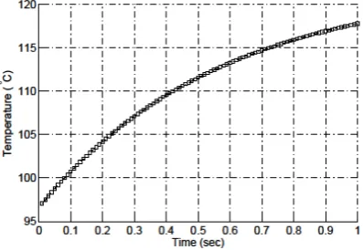
prediction temperature results from Eq. 12 with time increasing, that interval is 0.01s. Since second derivative can describe the variation tendency of the temperature, the range of coefficient k can be widened compared with the method
[image:3.595.322.521.400.537.2]using first derivative and the predictive value will be more accurate in a wide range of time.
Fig. 2 Temperature prediction results from Eq. 12.
IV. HARDWAREIMPLEMENTATION
To realize temperature prediction units, hardware is adopted by using modular programming, which can avoid the effect of the predictive temperature computation on the application workload. The relation between the task workload, time, the flow and the predictive temperature can be analyzed in detail through these hardware modules. These modules are embedded in the routing unit of each NoC node. Main components of the prediction temperature unit as shown in Fig. 3.
The Data flow enter into the routing unit through router ports or local ports, at the same time, the data traffic v can be
counted for calculating the power consumption of the routing, i.e., Prouter, and the performance data which is usually
Fig. 3 The temperature prediction unit structural sketch map.
consumption, i.e., Pprocessor. The power consumption of each
node is associated with above two parameters. Therefore, in the power consumption detection module, the power consumption of the routing can be expressed as:
horizontal router
,router bit bit
P P d P v (13) where horizontal
bit
P
represents the power consumption of the link between horizontally adjacent routers whentransmitting one bit, and d is the length of the link between
adjacent routers, while router bit
P
denotes the power consumption of the router when transmitting one bit. Finally, the current power consumption can be computed as:
( )
0.
processor router
P t
P
P
(14)The temperature monitoring module is used for sensing the temperature of the current nodes, i.e., T(t0). Through (12) in
Section III, these above information of power and temperature can be used in temperature prediction computation module to derive the predictive temperature. According to the prediction temperature, routing controller can select an optimal transmission path, and then cross switch will send data to the selected output port.
V. EXPERIMENTSRESULTS
A.Experimental Environment
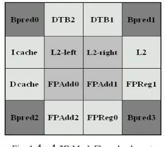
In this experiment, we conduct our experiments by using HotSpot 5.0 to demonstrate the effectiveness of our inference. HotSpot makes use of the duality that exists between the electrical and thermal properties of materials to model processor temperature, which is close to the actual value [23]. Therefore, the temperature achieved by HotSpot 5.0 is regarded as the actual temperature in this experiment. In order to compare the simulated results and the predictive temperature for simplicity, we divide the plane into 16 blocks averagely, i.e.,
4 4
2D Mesh, and make the assumption that power of all the blocks are equal. As the symmetry of the floorplan layout and the consistency of the power, these blocks have three symmetrical sections, as shown in Fig. 4. Therefore, only three blocks are chosen for the experiment, i.e., L2, L2-left and Bpred0. Various blocks are in different places, so the parameter b in (13) is differentfor each block which is chosen above [6]. By analyzing the actual data from HotSpot 5.0, in this work, we choose different b for above three blocks, i.e., bL2=0.21, bL2-left=0.18
and bBpred0=0.25.
Fig. 4
4 4
2D Mesh Floorplan layout.B. Experimental Results and Discussion
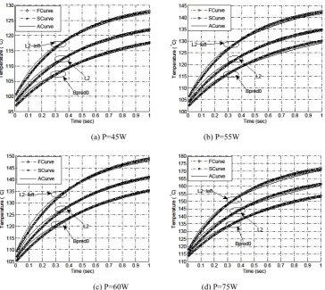
1) Prediction Window Length: We set the time interval as 0.1s and relax the time width to 3s. In addition, to discover the trends of temperature rise clearly and show the consistency of the trends, we intentionally select larger power levels which are 45W, 55W, 60W and 75W, respectively. Fig. 5 shows the temperature curves of the three blocks with these four different power levels. We also rebuilt the model deduced by first derivative [21] in this work to make comparison. The curves of each blocks in Fig. 5 are achieved by three different models, i.e., the model deduced by first derivative, the proposed model deduced by second derivative and the HotSpot software. And the curves can be simplified as FCurve, SCurve and ACurve which is achieved from the HotSpot for the above models, respectively. It can be seen from the figure that the deviation between the SCurve and the ACure is much smaller compared with the FCure with time increasing, which is due to the model deduced by second derivation takes nonlinear characteristic of temperature into consideration.
[image:4.595.343.512.287.438.2](a) P=45W (b) P=55W
[image:5.595.107.479.59.387.2](c) P=60W (d) P=75W
Fig. 5 Temperature prediction results achieved by three different methods with four power levels and the time intervals are 0.1s
(a) P=45W (b) P=55W
(c) P=60W (d) P=75W
Fig. 6 Temperature prediction results achieved by three different methods with four power levels and the time intervals are 0.01s.
[image:5.595.112.477.415.740.2]distinguishing value, i.e., 0.6% (about 0.7ºC). Moreover, all errors of each block are less than 0.6% in the optimal scope with the same power gradient. Then, we average these two sets of data respectively to achieve the final prediction windows, i.e., the prediction window of the model deduced by first derivative is [0s-1s], and that of the proposed model is [0s-2.6s]. It is obvious that the proposed model can increase the prediction time length at the same precision.
2) Prediction Accuracy: To further validate the accuracy of the proposed model in this paper, we modify the time interval to 0.01s and reduce the time length to 1s which is the prediction window length for the model deduced by first derivative. Fig. 6 shows the temperature curves of the three blocks within 1s, in which have 100 data points. The curves of each block are achieved by three different models as mentioned in Fig. 5. It can be seen from the figure that all the curves of the prediction temperature coincide well with the actual results.
In order to show the differences between these two models clearly, we also compare the errors between the prediction and actual temperatures of the FCurve with the errors of the SCurve. The results obtained through two models have few discrepancies within 1s, and the maximum difference of the error between these two models is about 0.0013 (about 0.16 ºC) at the same conditions, which is small enough to be negligible. Therefore, it can be concluded that, the accuracy of the proposed model keeps consistent with that of the model deduced by first derivative during this period.
VI. CONCLUSION
In this paper, from broadening the prediction time length prospective, we proposed a predictive thermal model based on the Thermal RC model combined with second derivative, which can describe the variation tendency of the temperature more clearly. We demonstrated that the proposed predictive thermal model provides good performance, which can increase the prediction range obviously with holding high accuracy. The strategy of information sharing based on multicast transmission will be investigated in our future work to realize the temperature information highly effective transmission.
ACKNOWLEDGMENT
This work is supported by the National Natural Science Foundation of China (Grant No. 61376025/61301111) and the Natural Science Foundation of Colleges and Universities of China's Jiangsu Province (Grant No. 13KJB510039).
REFERENCES
[1] M. Jabbar, A. M’zah, O. Hammami, and D. Houzet, “Exploration of 2D EDA tool impact on the 3D MPSoC architectures performance,” in Proc. 5th Asia Symp. Quality Electron. Design (ASQED), Aug. 2013, pp. 249–255.
[2] L. Carloni, P. Pande, and Y. Xie, “Networks-on-chip in emerging interconnect paradigms: Advantages and challenges,” in Proc. ACM/IEEE 3rd Int. Symp. Netw.-on-Chip (NoCs), May 2009, pp. 93–102.
[3] A. Kohler and M. Radetzki, “Fault-tolerant architecture and deflection routing for degradable NoC switches,”in Proc. ACM/IEEE 3rd Int. Symp. Netw.-on-Chip (NoCs), May 2009, pp. 22–31.
[4] P. Hamedani, S. Hessabi, H. Sarbazi-Azad, and N. Jerger, “Exploration of temperature constraints for thermal aware mapping of 3D networks on chip,” in Proc. 20th Euro. Int. Conf. Parallel, Distrib. Netw.-Based Processing (PDP), Feb. 2012, pp. 499–506.
[5] A.-M. Rahmani, K. Vaddina, K. Latif, P. Liljeberg, J. Plosila, and H. Tenhunen, “Design and management of high-performance, reliable and thermal-aware 3D networks-on-chip,” IET, Circuits, Devices Syst., vol. 6, no. 5, pp. 308–321, Sep. 2012.
[6] H. Wei, S. Ghosh, S. Velusamy, K. Sankaranarayanan, K. Skadron, and M. Stan, “Hotspot: a compact thermal modeling methodology for earlystage VLSI design,” IEEE Trans. Very Large Scale Integr. (VLSI) Syst., vol. 14, no. 5, pp. 501–513, May 2006.
[7] C. Addo-Quaye, “Thermal-aware mapping and placement for 3-D NoC designs,” in Proc. IEEE Int. Conf. Syst.-on-Chip (SoC), Sep. 2005, pp. 25–28.
[8] C. Zhu, Z. Gu, L. Shang, R. Dick, and R. Joseph, “Threedimensional chip-multiprocessor run-time thermal management,” IEEE Trans. Comput.-Aided Design Integr. Circuits Syst., vol. 27, no. 8, pp. 1479–1492, Aug. 2008.
[9] P. Budhathoki, A. Henschel, and I. Elfadel, “Thermal-driven 3D floorplanning using localized TSV placement,” in Proc. IEEE Int. Conf. IC Design Technol. (ICICDT), May 2014, pp. 1–4.
[10] D. Abdullah, W. Abdullah, N. Babu, M. Bhuiyan, K. Nabi, and M. Rahman, “VLSI floorplanning design using clonal selection algorithm,” in Proc. IEEE Int. Conf. Inform. Electron. Vision (ICIEV), May 2013, pp. 1–6.
[11] Y. Cheng, L. Zhang, Y. Han, and X. Li, “Thermal-constrained task allocation for interconnect energy reduction in 3-D homogeneous MPSoCs,” IEEE Trans. Very Large Scale Integr. (VLSI) Syst., vol. 21, no. 2, pp. 239–249, Feb. 2013.
[12] Y. Ge and Q. Qiu, “Task allocation for minimum system power in a homogenous multi-core processor,” in Proc. Int. Conf. Green Computing (GREENCOMP ’10), Aug. 2010, pp. 299–306. [13] Y. Cui, W. Zhang, and H. Yu, “Distributed thermal-aware task
scheduling for 3D network-on-chip,” in Proc. IEEE 30th Int. Conf. Comput. Des. (ICCD), Sep. 2012, pp. 494–495.
[14] X. Zhou, Y. Xu, Y. Du, Y. Zhang, and J. Yang, “Thermal management for 3D processors via task scheduling,” in Proc. IEEE 37th Int. Conf. Parallel Processing (ICPP ’08), Sep. 2008, pp. 115–122.
[15] C.-H. Chao, K.-Y. Jheng, H.-Y. Wang, J.-C. Wu, and A.-Y. Wu, “Trafficand thermal-aware run-time thermal management scheme for 3D NoC systems,” in Proc. ACM/IEEE 4th Int. Symp. Netw.-on-Chip (NOCS), May 2010, pp. 223–230.
[16] K.-J. Lee and K. Skadron, “Using performance counters for runtime temperature sensing in high-performance processors,” in Proc. IEEE 9th Int. Symp. Parallel Distrib. Processing, Apr. 2005, pp. 8–10. [17] A. Coskun, T. Rosing, and K. Gross, “Utilizing predictors for
efficient thermal management in multiprocessor SoCs,” IEEE Trans. Computer- Aided Des. Integr. Circuits Syst., vol. 28, no. 10, pp. 1503–1516, Oct. 2009.
[18] F. Zanini, D. Atienza, and G. De Micheli, “A control theory approach for thermal balancing of MPSoC,” in Proc. IEEE Asia South Pacific Design Autom. Conf.(ASP-DAC), Jan. 2009, pp. 37–42.
[19] P. Kumar and D. Atienza, “Neural network based on-chip thermal simulator,” in Proc. IEEE Int. Symp. Circuits Syst. (ISCAS), May 2010, pp. 1599–1602.
[20] I. Yeo, C. C. Liu, and E. J. Kim, “Predictive dynamic thermal management for multicore systems,” in Proc. ACM/IEEE 45th Design Autom. Conf. (DAC), Jun. 2008, pp. 734–739.
[21] K.-C. Chen, S.-Y. Lin, and A.-Y. Wu, “Design of thermal management unit with vertical throttling scheme for proactive thermal-aware 3D NoC systems,” in Proc. Int. Symp. VLSI Design, Autom., Test (VLSI-DAT), Apr. 2013, pp. 1–4.
[22] S. Wang and R. Bettati, “Reactive speed control in temperatureconstrained real-time systems,” in Proc. 18th Euro. Conf. Real-Time Syst., 2006, pp. 73–95.