Abstract— Currently, many control performance assessment
methods of cascade control loops are developed based on the assumption that all the disturbances are subject to Gaussian distribution. However, in the practical condition, several disturbance sources occur in the manipulated variable or the upstream exhibits nonlinear behaviors. In this paper, a general and effective index of the performance assessment of the cascade control system subjected to the unknown disturbance distribution is proposed. Unlike the minimum variance control index, an innovative control performance index is given based on the information theory and the minimum entropy criterion. The index is informative and in agreement with the expected control knowledge. To elucidate wide applicability and effectiveness of the minimum entropy cascade control index, a simulation problem and a cascade control case of an oil refinery are applied.
Index Terms — Cascade control; Minimum entropy;
Non-Gaussian; Performance assessment
I. INTRODUCTION
Starting from the end of the 1980s, a lot of statistical tools for monitoring the process performance were introduced [1]. These tools formed a new field called statistical process control, which utilized statistical methods to monitor the process variability and detect the presence of disturbance. However, they cannot evaluate whether the current control action is taken in an adequate working condition.
Like most of the controllers whose initial designs can meet its performance specifications, their performances can be deteriorated abruptly or gradually after long term operations. A study by Honeywell Process Solution indicated that almost 63% of all the control loops have poor performance ratings. The research on the control system performance assessment can be traced back to the 1960s and 1970s. Astrom (1967) and DeVries and Wu (1978) carried out the fundamental research [2,3]. In the literature of control loop performance assessments, the minimum variance control (MVC) had been widely used as a reference bound on the achievable performance since Harris (1989) proposed it [4]. The groundbreaking research has received increasing attention in the process control field. Then several research efforts have been focused on the evaluation of the control performance.
This work was sponsored in part by Ministry of Science and Technology, R.O.C. (MOST 103-2221-E-033-068-MY3).
J. Chen is with Department of Chemical Engineering, Chung-Yuan Christian University, Chung-Li District, Taoyuan, Taiwan 320, Republic of China (corresponding author to provide e-mail: [email protected]).
Z. Zhang and L. Zhang are with State Key Laboratory of Alternate Electrical Power System with Renewable Energy Sources, North China Electric Power University, Beijing 102206, China.
The performance assessment of SISO feedback control was extended to that of MIMO feedback control [5]. A generalized minimum variance as the performance assessment benchmark for the single loop control system was proposed [6]. When it comes to the performance assessment, cascade control has a significant advantage in improving the dynamic response performance and the anti-disturbance ability, but most of the research work in the past focused on applying advanced control algorithms to designing good controllers to improve cascade control quality. Sadasivarao and Chidambaram (2006) applied the genetic algorithm for tuning PID controllers of cascade control systems [7]. Padhan and Majhi (2012) proposed an improved cascade control structure with a modified Smith predictor for controlling open-loop unstable time delay processes [8]. There is not much research work on the performance assessment of cascade control in both the theories and applications. Ko and Edgar (2000) first derived the performance assessment of the classic cascade control loops based on MVC [9]. Chen et al. (2007) used the performance analysis to diagnose cascade control loop status [10].
So far a lot of past research on control performance assessment (CPA) assumed that the disturbances or the noises are subject to Gaussian distributions. This means that controlling the mean and the variance of the random variables was established. In fact, most industrial processes have difficulty meeting these prerequisites because of the mixture of different courses with Gaussian disturbances or other factors, resulting in misreporting the evaluation performance of the controlled process. Examples include a great variety of man-made noise sources, such as electronic devices, neon lights, relay switching noise in telephone channels and automatic ignition systems. For a system with non-Gaussian noise, the lower order statistics cannot provide enough information. That is, minimum variance is not a good benchmark for the cascade control loops with non-Gaussian disturbances. In despite of this fact, the performance assessment of cascade control systems with non-Gaussian noise has seldom been discussed in the open literature.
To extend MVC based CPA to the cascade control system with non-Gaussian disturbance, this paper presents a comprehensive minimum entropy methodology for the performance assessment of a cascade control loop. The paper is organized as follows: In Section 2, the conventional performance assessment for the cascade control system based on minimum variance control is reviewed. In Section 3, the cascade control performance assessment method based on minimum entropy control (MEC) criterion is proposed. In Section 4, case studies, including a simulation case and a cascade control loop from the industrial plant, are conducted
Entropy Information Based Assessment of
Cascade Control Loops
to show the advantages of the proposed method. Finally, in Section 5, conclusions are made.
II. CONVENTIONAL PERFORMANCE ASSESSMENT OF A CASCADE CONTROL SYSTEM
1
c
G Gc2 G2 G1
2( )
y k ()
1k y
0
sp y
2
L
G
2( )
a k a k1( )
1( )
u k u k2( )
1
L
[image:2.595.54.286.121.241.2]G
[image:2.595.306.546.525.662.2]Fig. 1. Cascade control system
Fig. 1 shows a discretized cascade control system with unity feedback. A cascade control loop consists of a primary loop and a secondary loop. These loops might also be referred to as the outer loop and the inner loop, respectively. The primary loop provides the secondary loop with a setpoint, or a target, for a process related to the primary control objective. The subscript, 1, in this figure refers to the primary control loop while the subscript, 2, refers to the secondary control loop. The subscript C of the transfer function denotes the controller and the subscript L of the transfer function denotes the disturbance filters. The unmeasured stochastic disturbances in the primary loop can equivalently be added at the output of the primary loop as well as of the secondary loop. y k1( ) and y k2( ) are the process outputs of the
primary loop and of the secondary loop at the sampling time
k. The outputs of the two loops are
1( ) 1 2( ) L1 1( )
y k G y k G a k
(1)
2( ) 2 2( ) L2 2( )
y k G u k G a k (2)
1( )
y k is the deviation variable from its set point and y k2( )
is the deviation of the secondary output from its steady-state value, which is required to keep the primary output at its set point. u k1( ) and u k2( ) are the manipulated variables which
are the outputs of the primary controller and of the secondary controller, respectively. a k1( ) and a k2( ) represent the
disturbance in the primary loop and in the secondary loop, respectively. The process transfer function in the primary
loop is * 1
1( ) 1( )
d
G q G q q with the time delay equal to d1,
and *
1( )
G q is the primary process model without any time delay. Similarly, for the secondary loop, * 2
2( ) 2( )
d
G q G q q
is the process transfer function in the secondary loop with time delay equal to d2 and
*
2( )
G q is the secondary process model without any time delay. The effects of all the unmeasured disturbances to the two loops are represented as disturbance filters GL1( )q and GL2( )q , both of which are
assumed to be a rational function of the backward shift 1 q , and they are driven by stochastic disturbances a k1( ) and
2( )
a k , respectively.
The minimum variance in a cascade control loop can be obtained by analyzing the system model and the estimated disturbance sequences. According to the transfer functions of the system, the primary output can be further decomposed as,
1 1 1
1 1 1 2 2
1 2 1 1 2 2
feedback_invariants
feedback_variants
( ) ( ) ( ) ( ) ( )
[ ( ) ( )]
d
d d
y k Q q a k S q q a k
M a k M a k q
(3)
where
* *
1 2 2 1 2 1 2 1
1
2 2 1 2 1 2
(1 )
1
c c c
c c c
R G G G G G G Q
M
G G G G G G
* *
2 2 2 2 2 1 1 2
2
2 2 1 2 1 2
(1 )
1
c c
c c c
T G R G G G G S
M
G G G G G G
The MV cascade controller can be obtained by simultaneously solving M10 and M2 0 . The
polynomials Q q1( ) and S q2( ) are feedback-invariant and
depend only on the disturbance characteristics. They can be represented by:
1 2 ( 1 2 1)
1 10 11 12 1( 1 2 1)
d d
d d
Q Q Q q Q q Q q (4)
1 2 ( 2 1)
2 20 21 22 2( 2 1)
d d
S S S q S q S q (5)
Thus, the feedback invariant term
1 1 1
1( ) ( )1 2( ) 2( ) d
Q q a k S q q a k consists of the first d1d2
terms of the moving-average model, and used as a benchmark measure of minimum variance control. When M1M20,
the primary output y k1( ) can achieve minimum variance.
And the value of the minimum variance is
1 2
2
1 1 1 2 2
1
0
var{ ( ) ( )}
d y mv
d d T
i i
i
Q a k S q a k
trace N N a
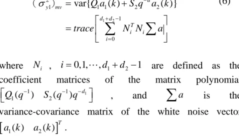
( ) (6)
where Ni , i0,1,,d1d21 are defined as the
coefficient matrices of the matrix polynomial
1
1 1
1( ) 2( )
d
Q q S q q
, and
a is thevariance-covariance matrix of the white noise vector
1( ) 2( )
Ta k a k .
The performance index of the cascade control system is defined as:
2 1
2 1
( y)mv mv
y
(7)
where (2y1)mv is the variance of the MVC output, and
2 1
y
control process under the condition that both disturbances are subject to the Gaussian distribution. Here a simple example is used to show the weakness of the minimum variance index for a dynamic system whose disturbance does not follow the Gaussian distribution:
1 1 2 1 1
2 1 2 1 2
0.6235 1
( ) ( 6) ( )
1 0.8368 1 0.8
0.3055 1
( ) ( 2) ( )
1 0.9482 1 0.98
y k y k a k
q q
y k u k a k
q q
(8)
(a)
0 100 200 300 400 500 600 700 800 900 1000 -10
-8 -6 -4 -2 0 2 4 6 8 10
y1
Time points
(b)
0 100 200 300 400 500 600 700 800 900 1000 -10
-8 -6 -4 -2 0 2 4 6 8 10
y1
[image:3.595.59.276.123.552.2]Time points
Fig. 2. Output responses of two different disturbances.
According to the engineering experience, the PI controller (Gc1) and the P controller (Gc2) in the outer loop and in the
inner loop are used:
1
1 1
0.2848 0.2568
1 c
q G
q
2 0.2
c
G
1( )
a k and a k2( ) are assumed to follow the -distribution.
The PDF of the -distribution can be represented by
1 1
( 1,1)
1
( , ) (1 ) ( )
( , )
a b
f x a b x x I x
B a b
(9)
where B( ) is the Beta function. The indicator function
( 1,1)( )
I x ensures that only the values of x in the range (-1, 1) have nonzero probabilities.
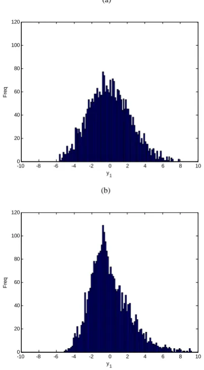
If the models are completely given and the two different unmeasured disturbances with non-Gaussian disturbances are applied to the inner and the outer loops respectively, the output responses under the same controller parameters are shown in Fig. 2. For easy visual comparisons, the corresponding distributions are shown in Fig. 3, and both variances are very close to the value of 5.5. From the observations in Fig. 3, Fig. 3(b) is sharper and narrower than Fig. 3(a); it seems that Fig.3(b) has better control performance. However, the MVC performance assessment indexes for Fig. 7(a) and Fig. 7(b) are 0.8072 and 0.7039 respectively, yielding the opposite conclusions. Due to the non-Gaussian disturbances, the conventional MVC performance assessment index would not provide correct information and may lead to wrong detection.
(a)
-10 -8 -6 -4 -2 0 2 4 6 8 10 0
20 40 60 80 100 120
Fr
e
q
y
1
(b)
-10 -8 -6 -4 -2 0 2 4 6 8 10 0
20 40 60 80 100 120
Fr
e
q
y
[image:3.595.322.524.297.662.2]1
Fig. 3. Output distributions of two different disturbances.
III. MINIMUM ENTROPY BASED ASSESSMENTS OF CASCADE CONTROL SYSTEMS
A. Entropy information analysis
as a measure of the information in a random signal [11]. Entropy is really a notion of self information provided by a random process about itself. Entropy has some great features. It has the property of convex, making it available to be the objective function of the optimization problem.
To characterize quantitatively a finite and discrete random
set X{ ,x x1 2,...,xn} , Shannon (information) entropy
( H( )X ) can be defined. The Shannon entropy is distinguished by several unique properties [12], but it is often convenient to introduce generalized Rényi entropies parametrized by a continuous parameter [13],
1
1
( ) ln
1 M
i i
H p
X (10)
where each element xiX has probability pi,i1, 2,...,n.
This means that pi , i1, 2,...,n , constructs a discrete
probability distribution
p1 p2 pM
which consistsof non–negative numbers summing to unity.
1
1 M
i i
p
. Rényi entropy is a generalization of Shannon entropy.B. Minimum entropy index for cascade control loop
In the real operation, the actual disturbance behavior is not known in advance. The results of the minimum variance based on the Gaussian disturbance would not be reasonable when the minimum variance index is applied to control processes with non-Gaussian disturbance distribution. Therefore, to assess a cascade control process with non-Gaussian disturbance, a minimum entropy based performance assessment is proposed. Entropy, as a general measure of uncertainty, has more physical relevance than the lower order statistics, such as the mean and variance of the arbitrary random variables. The variance of the output can merely measure the deviated degree from the mean, but it cannot comprehensively characterize the non-Gaussian disturbances. In this section, entropy, an alternative measure of uncertainty and dispersion, is used as an index to evaluate the control performance of the controller in cascade control systems.
For a cascade control process shown in Eqs.(1) and (2) with the unmeasured non-Gaussian disturbance a k1( ) and
2( )
a k , the entropy of the output y k1( ) can be written as
1 1 2
1 1 1 2 2 1 1 2 2
( ) ( d ( ) d d )
H y H Q a S q a M a M a q (11)
Because the non-Gaussian disturbance a k1( ) and a k2( )
are finite, stationary and mutually independent, the entropy of the output y k1( ) in Eq.(1) can be further decomposed into
1
1 2 1 1 2
1 1 1 1 2 2 2 2
( )
( , d d ) ( d , d d )
H y
H Q a M a q H S q a M a q
(12)
Lemma: Given two discrete random variables X and Y, defined on a common probability space, there is
0
H
( )
X
(13)and
( , )
max(
( ),
( ))
H
X Y
H
X
H
Y
(14) On the basis of Lemma,1 2
1 1 1 1 1 1
( , d d ) ( )
H Q a M a q H Q a (13)
1 1 2 1
2 2 2 2 2 2
( d , d d ) ( d )
H S q a M a q H S q a (14)
The lower bound of H y( )1 can be obtained, 1
1 1 1 2 2
( ) ( ) ( d )
H y H Q a H S q a (15)
The terms Q a1 1 and 1 2 2
d
S q a are the feedback invariant. The minimum entropy H y( )1 of cascade control can be obtained
if M1 M2 0,
1
1 1 1 2 2
1
1 1 2 2
( ) ( ) ( )
( , )
d me
d
H y H Q a H S q a
H Q a S q a
(16)
Now a new performance assessment index (me) can be
defined for the cascade control system with the non-Gaussian noises,
1
1
( )
( ) me me
H y
H y
(17)
where me is the ratio of the output of the minimum entropy
(H y( )1 me) to the current output of the minimum entropy
(H y( )1 ).
IV. EXAMPLES
A. Simulation of the cascade control system
In this case, the cascade control process with non-Gaussian disturbance is considered. a k1( ) and a k2( ) follow the same
-distribution as those in Section 2. The minimum entropy of y1 based on the models is 3.2920. Therefore, the MEC
performance index (Eq.(17)) is me 0.8669 and the theoretical one is TH 0.8675
me
. Thus, without the
B. Industrial cascade control loop
T
TIC
FIC
Q
r
Q Tr
T
[image:5.595.64.276.54.234.2]heating steam
Fig. 4. A temperature cascade control of the disturbance tower.
(a)
100 200 300 400 500 600 700 75
75.5 76 76.5 77 77.5 78
T
em
per
tur
e
Time points
(b)
100 200 300 400 500 600 700 75
75.5 76 76.5 77 77.5 78
Te
m
p
e
rt
u
re
[image:5.595.70.272.280.632.2]Time points
Fig. 5. Outputs of the primary loop of (a) Period 1and (b) Period 2
Oil refinery or petroleum refinery is an industrial process. The crude oil is processed and refined into more useful products, such as petroleum naphtha, gasoline, diesel fuel and so on. A multitude of separations is accomplished by distillation, but the most important and primary function in the refinery is the separation of crude oil into component fractions. To get the specific products, accurate temperature control is necessary. Hence, cascade control of temperatures is widely used in refinery. Fig. 4 shows a schematic diagram of a temperature cascade control to the distillation tower. To
ensure production running smoothly, the temperature T
should remain constant. And there is a regulating valve to control the heating steam flow Q. From the valve action to the temperature change, a lot of heat capacities are needed. It is better to adopt cascade control. Cascade control includes two closed-loop systems; the secondary loop is a flow control system while the primary loop is a temperature control system.
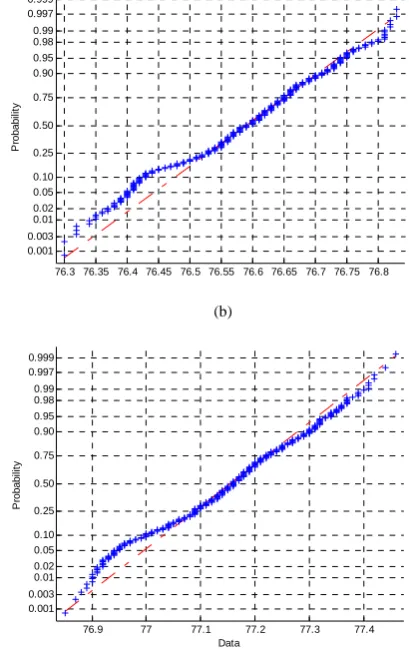
The cascade control loop from refinery in a local plant in Taiwan is used to test the proposed MEC method. Fig. 5 shows 2,000 measurements of the outputs for the primary loop in two different operating periods. The sampling time is 1 second. From the normal probability analysis shown in Fig. 6, obviously, the output data cannot be exactly fitted into a straight line in the normal probability plots. Thus, the underlying population of the two measurements is not exactly normal. Calculating the MVC index of the two periods,
1
0.0946 mv
and mv2 0.1966, apparently, these values are unreasonable.
(a)
76.3 76.35 76.4 76.45 76.5 76.55 76.6 76.65 76.7 76.75 76.8 0.001
0.003 0.01 0.02 0.05 0.10 0.25 0.50 0.75 0.90 0.95 0.98 0.99 0.997 0.999
P
robabi
li
ty
(b)
76.9 77 77.1 77.2 77.3 77.4 0.001
0.003 0.01 0.02 0.05 0.10 0.25 0.50 0.75 0.90 0.95 0.98 0.99 0.997 0.999
Data
P
robab
ilit
y
Fig. 6. Normal probability plots of the output of (a) Period 1 and (b) Period 2 for the industrial cascade control loop.
[image:5.595.320.525.332.657.2]the collected data, and the delays of the primary loop and the secondary loop are 6s and 1s time units respectively. Then with the MEC based identification method, the ARMAX model can be obtained and the disturbance can be estimated. Fig. 7 shows the estimated disturbance distributions of Period 1 and Period 2, respectively. In Period 1, with the estimated disturbance sequences and the model parameters, the minimum entropy of the primary loop output is found to be 2.3109. The MEC index is 1
0.8657 me
. Likewise, in Period 2, the MEC performance assessment index is 2
0.6307
me
. From the analysis, the cascade control system in Period 1 performs better.
(a)
-0.10 -0.08 -0.06 -0.04 -0.02 0 0.02 0.04 0.06 0.08 0.1 5
10 15 20 25 30 35 40
a1
E
s
ti
m
at
ed F
req.
(b)
-0.10 -0.08 -0.06 -0.04 -0.02 0 0.02 0.04 0.06 0.08 0.1 5
10 15 20 25 30 35 40 45 50
a
1
E
s
ti
m
a
ted F
[image:6.595.71.268.224.573.2]req.
Fig. 7. Estimated disturbances of (a) Period 1 and (b) Period 2 for the industrial cascade control loop.
V. CONCLUSION
To continuously improve the process performance, the basic control loop must be constantly assessed. In the past, several different measures of CPA have been proposed, but the disturbance distribution is assumed to be normal. That is, MVC performance assessment is effective in evaluating the healthy degree of the cascade control system with Gaussian disturbances, but it fails when the system has non-Gaussian distribution. As the variance, a second order statistic is not sufficient to be a benchmark of the cascade control system with unknown disturbances. The contribution of this work is a reliable and general algorithm that allows one to estimate CPA for the controlled system with non-Gaussian
disturbance. The proposed method also works well even in the case of Gaussian disturbance. The proposed MEC based CPA is the Renyi’s quadratic entropy of the output under the minimum entropy control loop. The entropy canbe used to measure many other characteristics of the random disturbance, such as similarity, equality, disorder, and so on; so it is good for a performance criterion. Like MVC, when there is no set point change, the output under closed loop control can be devided into two terms, the feedback invariant entropy term and the feedback variant entropy term. The feedback invariant entropy term depends only on the disturbance characteristics rather than the function of the process model or the controller. The entropy canbe used to measure many other characteristics of the random disturbance, such as similarity, equality, disorder, and so on; so it is good for a performance criterion. The proposed MEC performance is more useful in practical processes. From the analysis results of the simulation and the real plant data, the proposed MEC-based CPA method presents better generality and accuracy in practical processes.
REFERENCES
[1] V. Venkatasubramanian, R. Rengaswamy, S. N. Kavuri and K. Yin, “A review of process fault detection and diagnosis: Part III: Process history based methods,” Comput. Chem. Eng. 27, pp.327-346, 2003. [2] K. J. Astrom, “Computer control of a paper machine-an application of
linear stochastic control theory,” IBM Journal, 11, pp.389-405, 1967. [3] W. DeVries and S. Wu, “Evaluation of process control effectiveness
and diagnosis of variation in paper basis weight via multivariate time-series analysis,” IEEE Trans. Autom Control, 23, pp.702-708, 1978.
[4] T. J. Harris, “Assessment of control loop performance,” Can. J. Chem. Eng., 67, pp.856-861, 1989.
[5] T. J. Harris, F. Boudreau and J. F. MacGregor, “Performance assessment of multivariable feedback controllers,” Automatica, 32, pp.1505-1518, 1996.
[6] M. J. Grimble, “Controller performance benchmarking and tuning using generalised minimum variance control,” Automatica, 38, pp.2111-2119, 2002
[7] M. V. Sadasivarao and M. Chidambaram, “PID controller tuning of cascade control systems using genetic algorithm,” J. Indian Inst. Sci., 86, pp.343-354, 2006.
[8] D. G. Padhan and S. Majhi, “Modified Smith predictor based cascade control of unstable time delay processes,” ISA trans., 51, pp.95-104, 2012
[9] B. S. Ko and T. F. Edgar, “Performance assessment of cascade control loops,” AIChE J., 46, pp.281-291, 2000.
[10] J. Chen, Y. Yea and C. K. Kong, “Diagnosis of cascade control loop status using performance analysis based approach,” Ind. Eng. Chem. Res., 45, pp.7540-7551. 2006
[11] R. V. Hartley, “Transmission of information1,” Bell Syst. Tech. J., 7, pp.535-563, 1928.
[12] A. I. Khinchin, Mathematical foundations of information theory (Vol. 434). Courier Dover Publications,1957.