Physiol. Meas.22(2001) 91–96 www.iop.org/Journals/pm PII: S0967-3334(01)19904-1
Adaptive mesh refinement techniques for electrical
impedance tomography
M Molinari1, S J Cox1, B H Blott2and G J Daniell2
1Department of Electronics and Computer Science, University of Southampton, Southampton
SO17 1BJ, UK
2Department of Physics and Astronomy, University of Southampton, Southampton SO17 1BJ,
UK
Received 4 December 2000
Abstract
Adaptive mesh refinement techniques can be applied to increase the efficiency of electrical impedance tomography reconstruction algorithms by reducing computational and storage cost as well as providing problem-dependent solution structures. A self-adaptive refinement algorithm based on ana posteriorierror estimate has been developed and its results are shown in comparison with uniform mesh refinement for a simple head model.
Keywords: nonlinear electrical impedance tomography, adaptive mesh refinement, h-refinement, p-refinement, efficiency, improved convergence
1. Introduction
Electrical impedance tomography (EIT) can provide images with well defined characteristics only when the full nonlinear reconstruction process is constrained by a property of the image such as its local smoothness, applied in parallel with the requirement to fit the data to within clearly defined statistical criteria (Blottet al1998, 2000). The finite element forward solution is a significant part of the computational cost of such a reconstruction (Yorkeyet al1987, Johnson and MacLeod 1994). This cost grows quickly when the image is subdivided into smaller and smaller elements to obtain an image whose accuracy is governed by the quality of the input data alone and not by the choice of discretization.
To overcome the problems involved in handling high-density discretizations, sparse matrix techniques have been applied in the past (Pinheiro and Dickin 1997) without taking into account that a proportion of the cost could be avoided by using meshes adapted to the problem.
We have developed an algorithm which automatically adapts to the reconstructed image by producing finer meshes in areas where there are sharp gradients in the EIT image. Typically, refinement is required at interfaces between regions with differing conductivities. Although adaptive meshing has not yet been applied to resistance or impedance modelling in a biomedical context, there exists some work on applications of adaptive mesh refinement (AMR) in modelling heart current sources (Johnson and MacLeod 1994)—a topic related to EIT.
We apply the auto-adaptive refinement method to the forward modelling problem and demonstrate that the method quickly reduces the number of nodes and elements so that the calculation converges much more rapidly to the true solution. In particular, to obtain the same accuracy as uniform refinement, the adaptive refinement reduces the number of elements by a factor of more than three, which yields up to an order of magnitude speed-up.
2. Methods
The basic equation of electrical impedance tomography in the case of imaging conductivityσ (or analogously for impedance imaging) is
∇·σ∇=0 on (1)
subject to the boundary conditions:
=0 onD σ∂∂n =jn onN (2)
whereand0 represent electrostatic potentials resulting from the injected current density
jnin the direction of the surface normaln, andDandNare the boundaries with Dirichlet or
von Neumann conditions, respectively. To solve equation (1) numerically, the problem domain
is subdivided into discrete finite elements. If insufficient elements are used, the choice of discretization will affect the accuracy of the potential distribution, and also the calculation of the Jacobian in the nonlinear reconstruction of the conductivities. It is therefore usual to refine the mesh globally to improve the accuracy of the solution across the whole domain.
However, it is in fact only necessary to refine the mesh where the error is large: the paradox is that the exact error is only known if the exact solution is available! We therefore use ana posteriorierror estimate, which is used to determine whether refinement of the mesh is required. Starting with an initially rather coarse quality mesh (Shewchuk 1996), we refine according to this estimator and adapt the mesh to give an accurate solution.
Error estimates for finite element analysis of elliptic problems have been extensively studied. We have chosen a residual-based energy norm estimator, which is robust (Salazar-Palmaet al 1998) and physically sound. It is obtained by multiplying equation (1) by an arbitrary weighting function and integrating by parts. We then obtain a measure for the error
e = exact −approx of the numerically approximated potential distributionapprox. Thea
posteriorienergy norm error||e||2
Eis estimated based on surface and lumped edge residuals
(rsurf, redge)of the intra-element and inter-element current densities within a two-dimensional
triangular mesh. The local error estimate,εlfor a single elementlwith areal, longest side
hland conductivityσlis computed as follows:
ε2 l =fsurf
h2 l
σlp
l r2
surfd+fedge
hl
σlp
k∈l
k⊂D
k r2
edged (3)
wherefsurfandfedgeare numerically estimated factors (Salazar-Palmaet al1998) and the sum
over edgesk in the second term runs over all elements (l) which do not have Dirichlet boundary conditions (D).prepresents the polynomial order of the basis function. The total error for the mesh can be approximated by summing the local estimates:
||e||2 E≈
Ne
l=1
ε2
l. (4)
Create initial mesh (solution domain)
Solve forward problem
Compute local & global error estimate
Check if global error estimate lower than limit
Refine elements with large error as ‘primary’ Measured data
Mark adjacent elements as ‘secondary’
Created further secondary elements ?
Refine secondary elements
Mesh refined only where necessary yes
yes no
[image:3.595.160.421.88.277.2]no
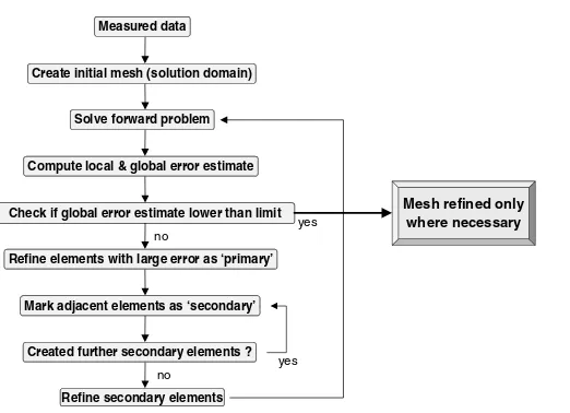
Figure 1. Steps in auto-adaptive mesh algorithm for solution of one instance of the forward problem.
(a) h-refinementconsists of subdividing elements into two or more elements;hrepresents the element size (Burnett 1987).
(b) p-refinementincreases the rate of convergence by using higher order interpolating basis functions on the elements (Zienkiewicz and Craig 1986).
(c) r-refinementrelocates the existing nodes of a mesh in a more appropriate fashion without adding any new nodes (Shepard 1985).
Efficient hybrids of these methods also exist, but can be complicated to implement. In this article, we focus on h-refinement of linear elements, which is both fast and adds relatively few additional elements and nodes to the mesh. p-refinement is an already commonly used improvement but produces larger matrices with increasing polynomial order. r-refinement requires modification of the mesh at each refinement stage but does usually not significantly improve the solution; however, it might be useful in time-dependent problems such as monitoring breathing, where the nodes of the mesh can follow predefined trajectories.
3. Auto-adaptive mesh algorithm
Figure 1 shows the steps in the adaptive meshing algorithm. We initialize the procedure with a coarse mesh and with the configuration of electrodes used. For reasons of simplicity we assume point-sized electrodes; however, the method works equally well for the complete electrode model (Somersaloet al1992). For each step in the forward solution of the EIT reconstruction, we estimate the local error using (3) and compute the global error using (4). If the global error estimate is larger than a pre-defined threshold, the refinement procedure is started. Otherwise, the refinement is complete. The refinement algorithm then starts by marking ‘primary’ elements, which are those with a local error estimate above a certain percentage of the maximum occurring local error (usually 40–50% for best efficiency).
Primary Secondary
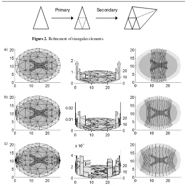
Figure 2.Refinement of triangular elements.
Figure 3. Example of auto-adaptive meshing for a head model showing bone, white matter and ventricles. Left, finite element mesh. Centre, local error estimates for each element inz-direction. Right, potential distribution in the region of interest for (a) the initial mesh, (b) after three refinement steps and (c) after seven refinement steps.
If we are using a fully nonlinear reconstruction algorithm (Blottet al2000), then the mesh refinement steps form a natural part of the iterative solver.
4. Results
Figure 4. Material gradient-dependent mesh refinement provides higher resolution at material boundaries (for example for smoothing constraints).
0.01 0.1 1 10
100 1000 No. of Elements 10000
G
loba
l Er
ro
r Es
ti
ma
te
adaptive
uniform
100 sec 0.010 sec
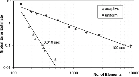
Figure 5.Comparison of error estimates for adaptive and uniform refinement for the head example.
Figure 4 shows the method being applied where we refine the mesh at boundaries between materials with significantly differing conductivities. In a practical application of our technique, it would be desirable to combine both strategies to yield an accurate solution, which can give good resolution of material boundaries.
If the image contains materials with differing conductivities, we can replace the error estimate, which determines when elements are refined, with one which refines elements based on the gradient of the reconstructed conductivity. This allows such boundaries to be more sharply resolved.
In figure 5 we show the performance benefits of our approach, by comparing the convergence of our method with a uniform refinement strategy. The adaptive algorithm requires only a small fraction of the number of elements/nodes in the uniformly refined mesh to achieve a given global error estimate. In particular, to attain a global error of 0.1 requires 300 elements and 0.01 s using the adaptive technique compared to 7000 elements and 100 s of computer time for the global refinement strategy. Since the solution of the forward problem scales with order betweenN1.46andN2, whereNis the number of nodes, reducingN saves both computation
[image:5.595.159.388.319.447.2]Whilst there are many benefits of the adaptive refinement procedure, a number of numerical issues can arise. For example, the method for subdividing the elements has to be chosen in a way to avoid degenerate elements of high aspect ratios (small angles) and subsequent incorrect solutions (Salazar-Palmaet al1998). In addition, non-smooth transitions between regions of low and high mesh densities are likely to produce less accurate results (Burnett 1987).
Our results were obtained on a 500 MHz AMD Athlon PC running Windows NT 4.0; the code is written in C++ and compiled using MS Visual C++ 6.0.
5. Conclusions and further work
We have developed an efficient adaptive mesh refinement algorithm and applied it to improve the performance of EIT reconstruction algorithms by reducing both computational and storage requirements. We demonstrate its application to imaging of a section through the head and show that (i) the accuracy of the forward solution is improved using considerably fewer elements than a global refinement strategy and (ii) the resolution of interfaces between materials with differing conductivities is improved.
Our results indicate that it is possible to reduce the number of nodes required by at least a factor of three to obtain an accurate image reconstruction, over a uniform refinement strategy. This results in at least an order of magnitude improvement in the speed of the forward problem and increases the feasibility of performing fully nonlinear reconstructions for complex large-scale biomedical problems in real-time using standard PC technology. Future work will integrate our method into a full nonlinear solver for 3D reconstruction.
Acknowledgments
We thank J Shewchuk for the meshing program TRIANGLE. MM is grateful to EPSRC for funding.
References
Blott B H, Cox S J, Daniell G J, Caton M J and Nicole D A 2000 High fidelity imaging and high performance computing in nonlinear EITPhysiol. Meas.211–7
Blott B H, Daniell G J and Meeson S 1998 Nonlinear reconstruction constrained by image properties in EITPhys. Med. Biol.431215–24
Burnett D S 1987Finite Element Analysis, from Concepts to Applications(Reading, MA: Addison-Wesley) Johnson C R and MacLeod R S 1994 Nonuniform spatial mesh adaption usinga posteriorierror estimates: applications
to forward and inverse problemsAppl. Numer. Math.14311–26
Pinheiro P A T and Dickin F J 1997 Sparse matrix techniques for use in electrical impedance tomographyInt. J. Numer. Methods Eng.40439–51
Salazar-Palma M, Sarkar T K, Garcia-Castillo L E, Roy T and Djordjevic A 1998Iterative and Self-Adaptive Finite Elements in Electromagnetic Modelling(Norwood: Artech)
Shephard M S 1985 Automatic and adaptive mesh generationIEEE Trans. Magn.212484–89
Shewchuk J R 1996 Triangle: engineering a 2D quality mesh generator and Delaunay triangulator1st Workshop on Applied Computational Geometry (ACM)pp 124–33 (http://www.cs.cmu.edu/∼quake/triangle.html) Somersalo E, Cheney M and Isaacson D 1992 Existence and uniqueness for electrode models for electric current
computed tomographySIAM J. Appl. Math.521023–40
Yorkey T J, Webster J G and Tompkins W J 1987 Comparing reconstruction algorithms for electrical impedance tomographyIEEE Trans. Biomed. Eng.34843–52