Evaluation of Multi part Models for Mean Shift Tracking

Evaluation of Multi-Part Models for Mean-Shift Tracking

Darren Caulfield

, Kenneth Dawson-Howe

Graphics, Vision and Visualisation Group

School of Computer Science and Statistics

Trinity College Dublin, Ireland

{Darren.Caulfield, Kenneth.Dawson-Howe}@cs.tcd.ie

Abstract

Mean-shift tracking is a data-driven technique for track-ing objects through a video sequence. We propose an inno-vation to mean-shift tracking that combines the background exclusion constraint with multi-part appearance models. The former constraint prevents the tracker from moving to regions where no foreground objects are present, while the multi-part nature of the models enforces a spatial structure on the tracked object. We also use a simple formula to de-termine the scale of the object in each video frame, and note the importance of setting an appropriate convergence con-dition. An evaluation of our proposed tracker and several existing trackers is performed using a ground truth dataset. We demonstrate that our innovation yields more accurate tracking than existing mean-shift techniques.

1. Introduction

Since its introduction in 2000 mean-shift tracking has attracted much attention in the computer vision community [2, 4, 5]. As a bottom-up, or data-driven, technique it per-mits regions of an image to be tracked over time without the need to specify complex motion or appearance models. A simple colour histogram is used to encode the appearance of the object to be tracked, while a spatial kernel enforces a degree of structure on the histogram.

Although mean-shift tracking is popular due to its rela-tive simplicity and computational efficiency, it suffers from a number of weaknesses: it is prone to distraction by other objects similar to the one being tracked; it does not cope well with changes in the scale of the object; and it lacks a mechanism for encoding the spatial layout of the colours the object. To date various researchers have attempted to ad-dress these problems. Zhaoet al. [12] have used the

back-∗_{This work was in part supported by a grant from the Irish Research}

Council for Science, Engineering and Technology: funded by the National Development Plan.

ground exclusionconstraint to make the tracker favour re-gions that are dissimilar to the background. Collins [1] has developed a method for selecting the appropriate scale for the tracker in each frame when the object’s size is changing. In order to enforce a particular spatial structure on the object various multi-part models have been proposed [6, 8, 11].

We have developed a mean-shift-based tracker that utilises both the background exclusion constraint and multi-part appearance models. We have also performed an evalua-tion of various trackers against a ground truth dataset, which demonstrates that our proposed innovation yields more ac-curate tracking of its target object. In order to deal with the changing size of the objects as they move through the scene we use a simple formula that relates an object’s size to its position in the image. We also note that one of the parame-ters used in mean-shift tracking – the convergence condition – critically affects a tracker’s performance.

The remainder of this paper is organised as follows: sec-tion 2 describes previous research into mean-shift tracking, including multi-part models and background exclusion. In section 3 we present our method of combining these two elements in a single tracker, while section 4 details the for-mula used to select the object’s scale at each frame. Section 5 describes the various trackers whose performance we as-sess and the metrics used in the evaluation. Finally, section 6 presents the results and draws conclusions about the track-ers.

2. Related research

2.1. Basic mean-shift tracking

Mean-shift, or kernel-based, tracking tries to find the area of a video frame that is both (a) most similar to a pre-viously initialised model and (b) close to the tracker’s lo-cation in the previous frame. By applying the technique to each video frame in sequence a region can be tracked over time. The method was first presented by Comaniciu in 2000

[2, 3]. The tracking begins with an object model being cre-ated from the region in the first frame. The probability den-sity function (pdf) of the region to be tracked (themodel) is represented by a histogramq= {qu}u=1...mwhere, for each histogram binu,

qu=C n

i=1

k

x_i2

δ[b(x_i)−u] (1)

In this equationkis a kernel function that gives more weight to pixels at the centre of the model, andC is a normal-ising constant that ensures that all of the elements of the histogram sum to 1 (there arenpixels in the model). The functionδis the Kronecker delta andbis a histogram bin-ning function for each pixel locationx_i. Similarly, the pdf of the candidate regionp(y) ={pu(y)}u=1...mat location yis given by

pu(y) =Ch nh

i=1

k

y−_hxi 2

δ[b(x_i)−u] (2)

wherehis the kernel bandwidth, which determines the size of the candidate region. It is useful to think of u as a colour, but the histograms could actually represent any fea-ture space, e.g edge magnitudes or oriented gradients. The indexiranges over each pixel in the tracked region.

Central to the operation of mean-shift is the weighting

wifor each pixel:

wi= m

u=1

qu

pu(y0)δ[b(

x_i)−u] (3)

which is derived from the Bhattacharyya similarity mea-sure. (y₀is the location of the candidate region in the previ-ous frame.) As in [3] we use an Epanechnikov kernel fork, so that the new locationy₁for the candidate region is found simply as

y₁= nh

i=1xiwi nh

i=1wi

(4)

Mean-shift is an iterative procedure, so the above formula must be applied until convergence. The tracker is consid-ered to have converged if the (x,y) locations returned by two successive iterations are separated by less than a particular threshold.

2.2. Multi-part models

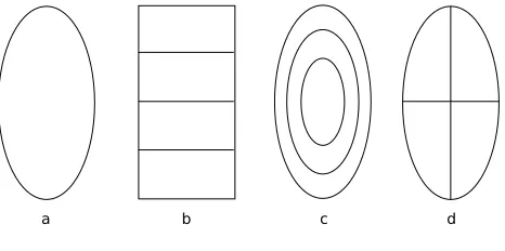
Both Maggioet al.[6] and Donget al.[11] have devel-oped multi-part models that retain much of the structure of the basic histogram (equation 2). Dong divides the region to be tracked into concentric ellipses (figure 1) and adds an extra dimension to the histogram to encode this spatial

structure:

pu,v(y) =

Cp ni=1p k

y−xi

hp

2

δ[bu(xi)−u]δ[bv(xi)−v] (5) whereu = 1...mare the colours (as before) andv= 1...n

are the ellipses. This results in a modification of equation 3 for calculating the weights:

wi= m

u=1 n

v=1

qu,v

pu,v(y0)δ[bu(xi)−u]δ[bv(xi)−v] (6) while the optimisation formula (equation 4) remains un-changed.

Although Maggio does not derive the equations explic-itly, his approach is very similar to Dong’s. However, Mag-gio’s tracker can be used to create models with regions that overlap.

Parameswaran’s multi-part model [8] has a different for-mulation to the others: a separate kernel is associated with each region of the model. For comparison we have included this tracker in our evaluation (section 5).

Figure 1. Spatial division of models for each tracker: (a) basic tracker (b) Parameswaran’s (c) Dong’s (d) our implementation of Maggio’s tracker

2.3. Background exclusion

Various authors have attempted to exploit background models of the scene to improve the performance of mean-shift tracking. Zhaoet al. [12] and Porikliet al.[10] have both modified the pixel weights (equation 3) to take account of the appearance of the background:

pixel in the background model. The foreground weightwf_i

is calculated as in equation 3, but the background weightwb i takes on a more complex form:

wb

i = mu=1

du(y0)

pu(y0)δ[bf(xi)−u]

+pu(y0)

du(y0)δ[bb(xi)−u]

(8)

whered(y) = {du(y)}u=1...mis the colour histogram of the corresponding region in the background model.

The incorporation of the background exclusion term makes the tracking appreciably more robust and improves its localisation (its positioning on an object).

3. Combining background exclusion with

multi-part models

We propose an enhancement of the basic mean-shift tracker that is analogous to the work of Pérezet al. in the area of particle filters [9]. The goal is to create a mean-shift tracker the has both of the following properties:

• multi-part appearance model: the model to be tracked should be represented by a number of histograms, so that some element of the spatial layout of the object to be tracked is recorded

• background exclusion:. the tracked region should look similar to the model but different to the corresponding region in the empty background scene

We achieve the above aims by combining the background exclusion tracker of Zhao with the multi-part models of Maggio and Dong.

In Pérez’s work the likelihood of a candidate regionp(y) at locationygiven the modelqis found using the expres-sion

exp−λD2[q,p(y)] (9) whereD is the Bhattacharyya distance. For a multi-part model withJ regions the expression becomes

exp−λ

J

j=1

D2[q_j,p_j(y)] (10)

and when a background modeld(y)is available Pérez uses

exp−λD2[q,p(y)]−D2[d(y),p(y)] (11) Expression 11 has a very similar form to that used by Zhao et al. [12] to exploit “background exclusion” in mean-shift tracking (section 2.3):

L(y) =λfD(q,p(y))−λbD(d(y),p(y)) (12)

We modify Zhao’s formula to allow the object, candidate and background models to haveJregions:

L(y) =λf J

j=1

D(q_j,p_j(y))−λb J

j=1

D(d_j(y),p_j(y))

(13) The weight wi for the entire expression on the right-hand side is still given by equation 7. However,wf_i is now calcu-lated as the sum overJregions:

wf_i =

J

j=1

Cjwi,jf δ[bj(xi)−j] (14)

whereCj is a normalising constant and wi,jf is found ac-cording to equation 6. Note that equation 14 accommodates overlapping regions in the multi-part model. The new ex-pression forwb

i with multi-part models can be derived in a similar manner.

4. Scale adaptation for tracked objects

There is currently no known application-independent way to adapt the scale of the trackers to accommodate changes in the size of the object being tracked [1]. For this reason we have decided to exploit the application-specific constraints available to us in order to provide an explicit scale for the trackers at every frame. Because the videos we process are recorded by a camera located some distance above the ground, every object’s apparent height is a linear function of its lowest image row (see figure 2). For an ob-ject whose initial image row isy1and whose initial size is

assumed to be1, its sizesat image rowyis found simply according to

s= 1 +(y−y1)∗scale_adaption_factor

image_height (15)

where scale_adaption_factor<1is the factor by which the object shrinks as it moves away from the camera (from the bottom of the image to the top). This factor is a constant across all objects for a given camera setup. By adapting the scale in this deterministic manner we can avoid the prob-lems that other techniques introduce.

5. Evaluation

5.1. Trackers

Figure 2. Scale of an object can be deter-mined as a linear function of its lowest image row

• Basic tracker: Comaniciu’s original mean-shift tracker (section 2.1) [3]

• BG exclusion: Zhao’s background exclusion tracker (section 2.3) [12]

• Parameswaran multi-part [8]

• Dong 3-circle multi-part (section 2.2) [11]

• Maggio 4-quadrant multi-part

• Combined 3-circle: our proposed innovation – com-bining background exclusion with Dong’s multi-part model (section 3)

• Combined 4-quadrant: another version of our pro-posed innovation – combining background exclusion with Maggio’s multi-part model

5.2. Convergence condition

We have discovered that the value of the threshold used in the convergence condition of the mean-shift tracker can have a critical effect on its performance. To date, this has not been discussed in the literature. We have found that the default value of 1 pixel (as recommended by Comaniciu in [3]) is suitable for the basic tracker, but causes the multi-part models to perform very poorly. It appears that the steps taken by these trackers at each iteration are smaller than this value, and so a 1-pixel threshold causes the tracker to cease “hill-climbing” prematurely. A value of 0.25 pixels improves the performance significantly.

5.3. Metrics for single runs

We have evaluated each tracker’s performance with re-spect to the ground truth bounding boxes of the CAVIAR dataset1. Sample frames from the videos with ground truth

1_{The datasets come from the EC Funded CAVIAR project/IST}

2001 37540, found athttp://homepages.inf.ed.ac.uk/rbf/

CAVIAR/

Figure 3. Frames of various trackers in oper-ation. The red rectangle shows the ground truth bounding box and the ellipses denote the positions of the trackers (red: basic; green: BG exclusion; blue: Parameswaran).

data and the trackers’ positions overlaid are shown in fig-ure 3. We have used a metric from the Video Perfor-mance Evaluation Resource(ViPER) system [7] called the “dice coefficient” to evaluate the frame-by-frame degree of overlap between the ground truth bounding box and each tracker’s bounding box (figure 4). The dice coefficient (2∗shared_area/area_sum) is a symmetric measure and so is less skewed by excessively large tracker bounding boxes than simple overlap measures.

A second metric that we have used measures each tracker’s positional accuracy on a frame-by-frame basis (figure 5). It is simply the distance of the tracker centroid from the ground truth centroid. The values of these metrics can be plotted for each frame in a single run of the tracker.

5.4. Aggregate metrics over multiple runs

In order to more thoroughly explore the performance of the trackers we have aggregated the above frame-by-frame metrics into two single numbers for each run of the tracker. This allows us to evaluate each tracker’s performance over multiple runs, where each run is initialised with a different model.

We display metrics of this kind as box plots, e.g., figure 6, with each column representing a different tracker. The “boxes and whiskers” show the distribution of the data over multiple runs. The top and bottom of the blue box mark the upper and lower quartiles, respectively, while the whiskers extend for 1.5 quartiles in each direction. The median of the data is marked by a red line, and outliers are shown as red crosses. The “notch” in each blue box delimits the 95% confidence interval. If the notches for two trackers do not overlap we can assert that there is a statistically significant performance difference between them.

6. Results and conclusions

700 800 900 1000 1100 1200 1300 1400 0.5

0.6 0.7 0.8 0.9 1

Frame number

Dice coefficient (normalised overlap)

Basic

Background exclusion Parameswaran

700 800 900 1000 1100 1200 1300 1400 0.5

0.6 0.7 0.8 0.9 1

Frame number

Dice coefficient (normalised overlap)

Dong 3−circle Maggio 4−quadrant Combined 3−circle Combined 4−quadrant

Figure 4. Dice coefficient for a single run of all seven trackers

over a single run where the woman being tracked is never occluded. Qualitatively, the performance of the the basic, background exclusion and Parameswaran trackers is below that of the others.

We have run the trackers multiple times with different models to track. (In each run the same object is being tracked; we have simply used different frames to initialise the model.) The multiple runs allow us to extract aggre-gate statistics, which are shown in figure 6. We can see that the two trackers that implement our proposed innova-tion (“combined 3-circle” and “combined 4-quadrant”) dis-play a small but statistically significant improvement over all other trackers.

Table 1 presents the lost-track performance of the trackers for a variety of scenarios: “unoccluded”; “quarter-off target” and “half-“quarter-off target”, where we deliberately initialise the tracker inaccurately (not centred on the person); and three scenarios featuring occlusion (see figure 7). Looking at the first three rows of the table it is clear that only those trackers that use background exclusion can reliably cope with poor initialisation. In

7000 800 900 1000 1100 1200 1300 1400 5

10 15 20 25 30 35 40

Frame number

Centroid distance from ground truth (pixels)

Basic

Background exclusion Parameswaran

7000 800 900 1000 1100 1200 1300 1400 5

10 15 20 25 30 35 40

Frame number

Centroid distance from ground truth (pixels)

Dong 3−circle Maggio 4−quadrant Combined 3−circle Combined 4−quadrant

Figure 5. Centroid distance for a single run of all seven trackers

the presence of occlusions (last three rows) the results are inconsistent: the BG exclusion and combined 3-circle trackers appear to have comparable lost-track performance, as do Parameswaran and combined 4-quadrant. However, even in those scenarios where Parameswaran’s lost track percentage is much lower than for other trackers, its centroid distance and dice coefficient metrics are much worse than the “good” trackers (those based on background exclusion). We will investigate this paradoxical situation in our future work.

References

[1] R. T. Collins. Mean-shift blob tracking through scale space. InIEEE Conference on Computer Vision and Pattern Recog-nition, volume 2, pages 234–240, 2003.

Basic BG excl Param Dong Maggio 3−circ 4−quad 2

4 6 8 10 12 14 16

Average centroid distance (pixels)

Performance of each tracker (centroid distance) over maximum of 15 runs

Basic BG excl Param Dong Maggio 3−circ 4−quad 0.7

0.75 0.8 0.85 0.9

Average dice coefficient

Performance of each tracker (dice coefficient) over maximum of 15 runs

Figure 6. Aggregate performance of all seven trackers over 15 runs. Our trackers are la-belled “3-circ” and 4-quad”.

[3] D. Comaniciu, V. Ramesh, and P. Meer. Kernel-based object tracking. Pattern Analysis and Machine Intelligence, IEEE Transactions on, 25(5):564–577, 2003.

[4] Z. Fan, M. Yang, Y. Wu, G. Hua, and T. Yu. Efficient Op-timal Kernel Placement for Reliable Visual Tracking. Pro-ceedings of the 2006 IEEE Computer Society Conference on Computer Vision and Pattern Recognition-Volume 1, pages 658–665, 2006.

[5] G. Hager, M. Dewan, and C. Stewart. Multiple kernel track-ing with SSD. Computer Vision and Pattern Recognition, 2004. CVPR 2004. Proceedings of the 2004 IEEE Computer Society Conference on, 1:790–797, 2004.

[6] E. Maggio and A. Cavallaro. Multi-Part Target Represen-tation for Color Tracking. Image Processing, 2005. ICIP 2005. IEEE International Conference on, 1:729–732, 2005. [7] V. Mariano, J. Min, J. Park, R. Kasturi, D. Mihalcik, H. Li, D. Doermann, and T. Drayer. Performance Evaluation of Object Detection Algorithms. International Conference on Pattern Recognition, ICPR02, pages 965–969, 2002. [8] V. Parameswaran, V. Ramesh, and I. Zoghlami. Tunable

Kernels for Tracking. Proceedings of the 2006 IEEE

Com-Scenario/Tracker Basic BG

exclusion

P

aramesw

aran

multi-part

Dong

3-circle

Maggio

4

-quadrant

Combined

3-circle

Combined

4-quadrant

Unoccluded 0 0 0 40 7 0 0

Quarter-off target 0 0 20 20 47 0 0

Half-off target 73 0 93 87 100 0 0

Modest occlusion 17 47 13 27 10 53 10

Severe occl. 1 45 69 72 69 93 55 72

Severe occl. 2 91 76 47 68 94 74 38

Table 1. Percentage of tracker runs that ended in a lost track for various scenarios

Figure 7. Frames from the “modest occlu-sion” scenario (top row), and one frame from each of the two “severe occlusion” scenarios (bottom row).

puter Society Conference on Computer Vision and Pattern Recognition-Volume 2, pages 2179–2186, 2006.

[9] P. Perez, C. Hue, J. Vermaak, and M. Gangnet. Color-based probabilistic tracking. European Conference on Computer Vision, 1:661–675, 2002.

[10] F. Porikli and O. Tuzel. Multi-Kernel Object Tracking. Mul-timedia and Expo, 2005. ICME 2005. IEEE International Conference on, pages 1234–1237, 2005.

[11] D. Xu, Y. Wang, and J. An. Applying a New Spatial Color Histogram in Mean-Shift Based Tracking Algorithm.Image and Vision Computing New Zealand, 2005.