Energy Efficient Mapping and Scheduling for DVS Enabled Distributed Embedded Systems

Energy-Efficient Mapping and Scheduling for DVS Enabled

Distributed Embedded Systems

Marcus T. Schmitz and Bashir M. Al-Hashimi

Dept. of Electronics and Computer Science

University of Southampton

Southampton, SO17 1BJ, United Kingdom

{m.schmitz,bmah}@ecs.soton.ac.uk

Petru Eles

Dept. of Computer and Information Science

Link¨oping University

S-58183 Link¨oping, Sweden

[email protected]

Abstract

In this paper, we present an efficient two-step iterative synthe-sis approach for distributed embedded systems containing dy-namic voltage scalable processing elements (DVS-PEs), based on genetic algorithms. The approach partitions, schedules, and voltage scales multi-rate specifications given as task graphs with multiple deadlines. A distinguishing feature of the pro-posed synthesis is the utilisation of a generalised DVS method. In contrast to previous techniques, which ”simply” exploit available slack time, this generalised technique additionally considers the PE power profile during a refined voltage selec-tion to further increase the energy savings. Extensive experi-ments are conducted to demonstrate the efficiency of the pro-posed approach. We report up to 43.2% higher energy reduc-tions compared to previous DVS scheduling approaches based on constructive techniques and total energy savings of up to 82.9% for mapping and scheduling optimised DVS systems.

1. Introduction and Related Work

Modern embedded systems are often implemented as dis-tributed systems consisting of several processing elements (PEs), like programmable microprocessors, ASIPs, FPGAs, and ASICs. In reality, such embedded systems have to con-currently perform a multitude of complex tasks under a strict timing behaviour, given in the system specification. However, due to the various degrees of application parallelism, the PEs experience non-uniform workloads, resulting in idle intervals. Furthermore, the performance of the allocated architecture can often not be adapted perfectly to the application needs, turning out as slack between deadline and the real finishing time.

Dynamic voltage scaling (DVS) exploits such idle and slack times to reduce the power consumption [12, 14, 21]. This is done by conjointly changing the supply voltage and the opera-tional frequency during run-time, with respect to temporal per-formance requirements. Recent implementations of DVS pro-cessors have shown that voltage scaling can reduce the power consumption by up to 10 times when running real-life appli-cations [5]. Nevertheless, modern microprocessors make often use of gated clocks to switch off unused circuit parts during idle

times. Hence, the power consumption depends on the function carried out, resulting in non-uniform PE power profiles; this holds also for DVS-PEs [5]. It was shown in [14, 19, 23] that the consideration of the PE power profile during the voltage selection leads to further energy savings.

System level co-design is a methodology aiming to aid the system designers/architects to solve the difficult problem of finding the ”best” suitable implementation for a system spec-ification. Three important co-synthesis steps are: a) Mapping: Determining the assignment of computational tasks to PEs and data transfers to communication links (CLs), b) Scheduling: Determining the execution order (sequencing) of tasks mapped to PEs and communications to CLs, and c) Evaluation: De-termining the quality of the implementation candidate (timing feasibility, cost, power, area, etc.). Previous research in co-synthesis is extensive but has mainly focused on traditional architectures excluding issues related to power [15, 20, 26] or considered energy optimisation with components that are not DVS enabled [8, 16, 22]. This research will provide a valuable basis for the presented work. However, three recently proposed synthesis approaches for distributed systems have a close re-lationship to the problems we address in this paper. In [11], a DVS optimised schedule is derived using a constructive list scheduling technique with a dynamic re-calculation of task pri-orities based on average energy dissipation. If the found sched-ule does not meet the specified deadline, priorities of tasks on the critical path are increased and all tasks are re-scheduled. In [18], a mobility based list schedule is modified towards DVS utilisation by distributing slack time more evenly among the tasks of the system. A method for the identification of scaled supply voltages for distributed system was introduced in [3]. However, it focuses mainly on the voltage selection and its iter-ative nature results in undesirable high execution times, which can not be tolerated in the inner most loop of an iterative sched-ule and mapping optimisation. All these approaches are based on constructive scheduling heuristics and neglect the power profile information during the supply voltage selection.

search space of iterative optimisation methods, compared to constructive techniques, schedules with reduced energy dissi-pation are likely be found. Furthermore, the optimisation pro-cess is guided by a generalised DVS algorithm [23]. This volt-age scaling technique takes into account the PE power profiles during a refined voltage selection, leading to further energy re-ductions. In addition to the schedule optimisation, we employ a task mapping based on GA to push the distribution of tasks among the architecture towards energy-efficiency by abetting the exploitation of DVS. Overall, we concentrate here on the task mapping and scheduling aspects rather than on the voltage selction, which is explained in [23].

The presented work makes the following contributions: a) It is shown how iterative improvement mapping and schedul-ing algorithms can be effectively adapted to optimise system implementations towards an efficient utilisation of the DVS-PEs while meeting, at the same time, hard deadlines. This is done using a new two-step approach for scheduling and map-ping based on genetic algorithms (GAs). b) The outlined sched-ule optimisation is based on a DVS algorithm, which takes into account the PE power profiles, hence, leading to further energy savings. c) To illustrate the efficiency of the proposed approach, a comparative study is presented, comparing our results with two recently published synthesis approaches [11, 18], which are based on constructive list scheduling heuristics and neglect the PE power profiles. This further includes a quantitative com-parison between a variable-voltage system and a multi-voltage system, which demonstrates the efficiency of the proposed tech-nique also for multi-voltage processors.

The remainder of this paper is organised as follows: Prelim-inary aspects are introduced in Section 2. Section 3 describes our synthesis approach in detail which then, in Section 4, is extended to multi-voltage systems. In Section 5 we present ex-tensive experiments and comparisons with the results produced by other approaches. We conclude in Section 6.

2. Preliminaries

2.1. Specification and Architectural Model

In this work, we consider that a multi-rate application is spec-ified as a set of communicating tasks, represented by a task graph GS(

T

,

C

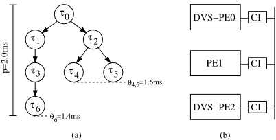
). This (hyper) task graph might be the combi-nation of several smaller task graphs, capturing all task activa-tions for the hyper-period (LCM of all graph periods). Fig. 1(a) shows a task graph example. Each nodeτ∈

T

in these graphs represents a task, an atomic unit of functionality to be executed without preemption. A node might inherit a hard deadlineθ, which must be met at run-time in order to ensure correct func-tionality. Edgesγ∈

C

in the task graph denote precedence con-straints and data dependencies between tasks. If two tasks,τi andτj, are connected by an edge, then the execution of taskτi must be finished before taskτjcan be started. Data dependen-cies inherit a data value, reflecting the quantity of information to be exchanged by two tasks. Further, each task graph has a specific period p, representing the time limit between two suc-cessive invocations. An implementation is only feasible when all timing and precedence constraints are fulfilled.

(b) (a)

CI

CI

CI

τ τ₄ τ₀

τ

p=2.0ms

DVS−PE2 DVS−PE0

PE1

τ₆

θ6

3 τ5

4,5

θ

τ₂ 1

=1.4ms

[image:2.612.347.548.50.152.2]

=1.6ms

Figure 1. Task graph and DVS architecture

The architectures we consider here consist of heterogeneous PEs, like general purpose processors, ASIPs, FPGAs, and ASICs. These components include state-of-the-art DVS-PEs. Furthermore, the PEs might employ lower level power manage-ment techniques, like gated clocks. An infrastructure of com-munication links, like buses and point-to-point connections, connects these PEs through communication interfaces (CIs), able to adapt to the different operational frequencies caused by scaling the DVS-PEs. An example architecture is shown in Fig. 1(b). The architecture is captured using a directed graph GA(

P

,

L

)where nodesπ∈

P

represent PEs and edgesλ∈

L

denote CLs.

Each task of the system specification might have multi-ple immulti-plementation alternatives, therefore, it can be potentially mapped to several PEs able to execute this task. If two com-municating tasks are accommodated on different PEs,πn and πmwith n6=m, then the communication takes place over a CL, involving a communication time and power overhead. For each possible task mapping certain implementation properties, like e.g. execution time, dynamic power dissipation, memory, and area requirements, are given in a technology library. These val-ues are either based on previous design experience or on esti-mation techniques such as those presented in [4, 17, 25]. This is not a trivial task and influenced by various parameters, e.g. the input data of the application. However, such techniques are essential to enable an effective co-synthesis, including the pre-sented approach.

2.2. Task Execution Order and DVS

The relation between dynamic power dissipation Pdyn, opera-tional frequency f , and supply voltage Vddis expressed by,

Pdyn=CL·N0→1·f·Vdd2 (1)

f =k·(Vdd−Vt)2/Vdd (2)

where CL denotes the load capacitance of the digital circuit,

N0→1represents the zero-to-one switching activity, k is a circuit

PE0

PE1

PE2

4

τ τ₅

0

τ τ1 τ2

3

τ

6

τ

(mW)

Slack P

t (ms)

E=71 Jµ

1 1.41.6

0.3 0.6 1

1

0.7 1.4 1.6

(a) Execution at nominal supply voltage Vmax

PE0

PE1

PE2

4

τ τ₅

0 τ τ1 τ2

τ₃ τ₆

P E=65.6 Jµ

1 1.4 1.6

1 0.3 0.6 (mW)

t (ms) 1.14 1.4 1.6

(b) Scaled execution with

[image:3.612.323.571.62.239.2]

Vdd3=2.08V and Vdd6=2.34V

Figure 2. Possible schedule not optimised for DVS

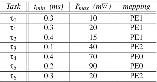
Fig. 2(a) shows a possible schedule for the tasks given in Fig. 1(a) executing at nominal supply voltage. The underlying architecture consists of two DVS-PEs (PE0, PE2) and one non-DVS-PE (PE1) connected through a bus, as given in Fig. 1(b). The nominal supply voltage Vmax and the threshold voltage Vt of PE0 and PE2 are Vmax=3.3V and Vt =0.8V , respectively, while PE1 runs all tasks at Vmax. For the sack of simplicity, the communications are neglected when discussing this particular example. The task execution times tminand power dissipations

Pmaxat nominal supply voltage are given in Table 1, which also shows the task mapping. According to these values, the energy

Task tmin (ms) Pmax (mW ) mapping

τ0 0.3 10 PE1

τ1 0.3 20 PE1

τ2 0.4 15 PE1

τ3 0.1 40 PE2

τ4 0.4 70 PE0

τ5 0.2 90 PE0

τ6 0.3 20 PE2

Table 1. Execution times, power dissipations, and mappings for the example task graph

dissipation corresponding to the given schedule can be calcu-lated as E =∑_τ∈T Pmax(τ)·tmin(τ) =71µJ. Considering the deadlines given in Fig. 1(a), it can be observed from Fig. 2(a) that the tasksτ3andτ6are eligible for scaling, sinceτ6finishes

at 1ms and it has a deadlineθ6=1.4ms, resulting in a slack

of 0.4ms. An extension of any other task can not be tolerated, since taskτ5has a finishing time equal to its deadline. By

scal-ing the schedule, usscal-ing our implementation of the generalised DVS technique (taking the PE power profile into account) pre-sented in [23], the voltage schedule shown in Fig. 2(b) can be produced, with tasksτ3andτ6executing at 2.08V and 2.34V ,

respectively. Thereby, the energy is reduced to 65.6µJ (using Equations (1) and (2)), a 7.6% reduction.

Now, consider a second feasible schedule at nominal supply voltage, as shown in Fig. 3(a), where the order ofτ1andτ2has

been exchanged. Since the mapping of the tasks has not been modified the dissipated energy remains E=71µJ. Observing

PE0

PE1

PE2 0

τ

4

τ τ₅

τ₁ τ₂

3

τ

6

τ

t (mW)P

Slack E=71 Jµ

0.7 1.1 1.3

1 0.7 0.3

(ms) 1.1 1.4 1.6

(a) Execution at nominal supply voltage Vmax

PE0

PE1

PE2 0

τ τ2 τ1

3

τ

6

τ

t (mW)P

E=53.9 Jµ

1.1 1.4 1.6 1 0.7 0.3

0.7 1.25

(ms) 4

τ τ₅

(b) Scaled execution with

Vdd4=2.74V and Vdd5=2.41V

Figure 3. Schedule optimised for generalised DVS

this schedule shows that only tasksτ4andτ5can be extended.

This is due to the slack time of taskτ5, which finishes execution

at 1.3ms while its deadline isθ5=1.6ms. Generating a voltage

schedule for this execution order of tasks results in the supply voltages Vdd4=2.74V and Vdd5=2.41V , using the same gen-eralised DVS technique as for the previous alternative. Hence, the energy is reduced to E=53.9µJ, an improvement of 24.1% compared to the 7.6% of the first schedule.

Although the schedule in Fig. 3(a) shows less slack than the one in Fig. 2(a), its energy reduction is significantly higher (with 16.5%). This is due to the particular power consumptions when executing the different tasks. The example demonstrates how important it is to take into consideration the power profiles during scheduling, in order to produce energy-efficient imple-mentations with DVS-PEs.

2.3. Genetic List Scheduling Algorithm

List scheduling algorithms (LS) make scheduling decisions based on task priorities. They maintain one or more ready list, which contain tasks ready to be scheduled. A static schedule is constructed by scheduling the ready task with the highest pri-ority as soon as the eligible PE becomes available. Thereby, the assignment of priorities defines the task execution order. Most traditional list scheduling approaches use various sophis-ticated algorithms to calculate these task priorities statically (before list scheduling) or dynamically (re-calculation after each scheduling step).

[image:3.612.52.298.62.236.2] [image:3.612.96.256.405.489.2]

qual-ity. c) There is a large freedom to trade-off between acceptable synthesis time and solution quality, as opposed to constructive techniques.

2.4. Problem Formulation

Using the common triplet notation for scheduling problems, our problem is described by Qm|prec|θj,fA,∑Esj, where Qm spec-ifies a multiprocessor environment, prec refers to a task model with precedence constraints,θjand fAare objectives capturing the deadline and area constraints, respectively.∑Es_jdenotes the additional objective to minimise the energy dissipation based on DVS. Therefore, the scheduling problem for DVS is to find an arrangement of the task execution order and mapping, such that the energy reduction through DVS-PEs is maximised and all specification constraints (timing, precedence, area, etc.) are met. A more detailed description of the synthesis problem, in-cluding the DVS problem, can be found in [24].

We make the assumption that the specified tasks are of suf-ficiently coarse granularity and that the PEs can continue oper-ation during the voltage scaling (as the case for the DVS pro-cessor in [5]), which allows to neglect of the scaling overhead in terms of power and time.

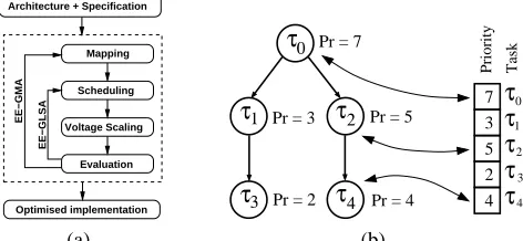
3. Energy-Efficient Synthesis Approach

In contrast to the GLSA based synthesis approach presented in [6, 10], our synthesis approach separates task mapping and scheduling into two nested optimisation steps; see Fig. 4(a).

• The GLSA for energy-efficiency, which produces an opti-mised sequencing of task executions (Section 3.1).

• A mapping optimisation based on GA, which distributes the tasks among the PEs of the architecture and, by this, decides on the execution time and power dissipation of each task (Section 3.2).

We have split these two steps due to the following reasons: a) The combination of list scheduling and mapping algorithms de-cide upon task priorities which task is to be scheduled next, but at this point it is not known where to execute the chosen task. Therefore, the execution time and power dissipation of the task are unknown as well. In this context, it is the duty of the sched-uler to make a ”greedy” mapping decision based on the power and time values with respect to the design objectives. How-ever, DVS influences the execution times and power dissipa-tions, hence, the mapping decision made upon the static values might proof to be wrong, especially from the energy reduction point of view. Separating the scheduling and mapping into two nested iterative optimisations overcomes this problem since the mapping is given before a schedule is constructed. b) Due to the constructive nature of list scheduling and mapping algorithms a solution is constructed one by one. This results in a greedy approach, which is likely to get trapped at low quality or in-feasible solutions in the presence of tight area and timing con-straints. A solution to overcome this problem was presented in [15]. However, this approach neglects issues related to power. By splitting the problem into two steps, we avoid this greedi-ness problem and can leverage the advantage of an increased search space, which is explored iteratively. Clearly, increasing

τ

0

τ

1

τ

2

τ

4

τ

3

τ

₀

1

τ

3

τ

τ

2

τ

₄

(a) (b)

Pr = 5

Pr = 4 Pr = 7

Pr = 3

Pr = 2

Priority Task

3 5 2 4 7 Architecture + Specification

Optimised implementation Evaluation Voltage Scaling

Mapping

Scheduling

EE−GLSA

[image:4.612.330.566.56.165.2]

EE−GMA

Figure 4. Presented energy-efficient synthesis ap-proach and task priority encoding into priority string

the search space results in high optimisation times, however, we show in Section 5 that these times are still reasonable.

3.1. Low-Energy Genetic List Scheduling Algorithm

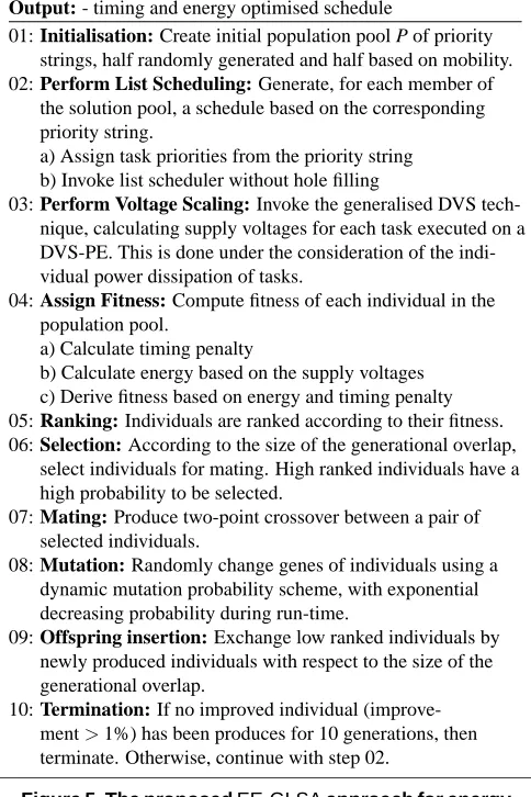
In this section, we give an overview of our DVS optimised GLSA for energy-efficiency, calledEE-GLSA. The algorithm generates an energy-efficient schedule of tasks and communi-cations for a given mapping. By imitating and applying the principles of natural selection and ”survival of the fittest” on a population pool of individuals, GAs are able to evolve (op-timise) solutions over several generations. In each generation a new population is evolved by mating (through crossover) the fittest individuals of the current population. Mutation provides an additional opportunity to enter unexplored regions of the search space by applying randomly changes to an individual. In our case, each individual is represented by a priority string (solution candidate) and each solution represents a schedule. Fig. 4(b) shows the encoding and the relations between prior-ity string and tasks. A description of theEE-GLSAis given in Fig. 5. The distinguishing features of this GA can be found in steps 02, 03, and 04, which are explained next. The remaining steps vary only slightly from common GAs, and more details on the functionality of GAs can be found elsewhere [9]. In step 02, for each priority string of the population a schedule is gener-ated by going through the following two steps: a) The priorities of each individual are assigned from the corresponding prior-ity string. b) Based on this priorprior-ity assignment, the execution order of tasks is determined by a list scheduling algorithm. In addition, our implementation of the list scheduler relies solely on the priorities to make scheduling decisions, i.e., no other optimisation technique (e.g. hole filling) is applied. Although such techniques can improve the timing behaviour by eliminat-ing idle periods, we dissociate from them since DVS exploits exactly these idle times.

implementa-EE-GLSA

Input: - task graph TG

- mapping and execution properties corresponding to the mapping

Output: - timing and energy optimised schedule

01: Initialisation: Create initial population pool P of priority strings, half randomly generated and half based on mobility. 02: Perform List Scheduling: Generate, for each member of

the solution pool, a schedule based on the corresponding priority string.

a) Assign task priorities from the priority string b) Invoke list scheduler without hole filling

03: Perform Voltage Scaling: Invoke the generalised DVS tech-nique, calculating supply voltages for each task executed on a DVS-PE. This is done under the consideration of the indi-vidual power dissipation of tasks.

04: Assign Fitness: Compute fitness of each individual in the population pool.

a) Calculate timing penalty

b) Calculate energy based on the supply voltages c) Derive fitness based on energy and timing penalty 05: Ranking: Individuals are ranked according to their fitness. 06: Selection: According to the size of the generational overlap,

select individuals for mating. High ranked individuals have a high probability to be selected.

07: Mating: Produce two-point crossover between a pair of selected individuals.

08: Mutation: Randomly change genes of individuals using a dynamic mutation probability scheme, with exponential decreasing probability during run-time.

09: Offspring insertion: Exchange low ranked individuals by newly produced individuals with respect to the size of the generational overlap.

10: Termination: If no improved individual

(improve-ment>1%) has been produces for 10 generations, then

[image:5.612.53.295.103.466.2]

terminate. Otherwise, continue with step 02.

Figure 5. The proposed EE-GLSA approach for energy-efficient schedules

tions. OurEE-GLSArelies on the following fitness function FS to achieve these goals,

FS=

∑

ε∈A

E(ε) !

| {z }

Energy diss. ·





1+

∑

τ∈Td DV_τ2

T2

HP



 

| {z }

Time penalty

(3)

where

A

=

T

∪

C

defines the set of all activities and

T

d rep-resents all hard deadline tasks. The first part of the equation is used to calculate the total dynamic energy dissipation of all activitiesε∈

A

. Based upon the type of activity, the energy dissipation can be calculate in the following way,

E(ε) =   

 

Pmax(ε)·tmin(ε)· V 2

dd(ε)

V2

max(ε) ifε∈

T

DVS Pmax(ε)·tmin(ε) ifε∈

T

\

T

DVS PC(ε)·tC(ε) ifε∈

C

where Pmaxand tminrefer to the power dissipation and execution time at nominal supply voltage, respectively, Vdd is the scaled

supply voltage,

T

DVS is the set of all tasks mapped to

DVS-PEs, and PC and tC denote the power and execution time of communication activities. The second part of the fitness func-tion (3) introduces a penalty factor due to deadline violafunc-tions of deadline tasks which are given by DVτ=max 0,tF(τ)−td(τ)

, where tF(τ)and td(τ)denote the finishing time and deadline of taskτ, respectively. THPis the hyper task graph period, used to relate the deadline violations. Squaring has been applied in order to assign a higher penalty to larger violations of imposed deadlines. The parameters of the GA where set as follows: The population pool consists of 25 individuals, the dynamic mu-tation probability is calculated as MP=max(0.15,1/exp(NS· 0.05))(NSis the current generation), and the generational over-lap is 50%.

3.2. Low-Energy Task Mapping Algorithm

The mapping step determines which PE carries out which task. Thereby, it determines the execution time and power dissipa-tion at nominal supply voltage. The mapping also specifies the area requirements of tasks in terms of bytes or gates, whether implemented as software or hardware. Obviously, due to the in-terrelation between scheduling and mapping, the distribution of tasks among the PEs has an influence on how well the allocated DVS-PEs can exploit their energy reduction possibilities.

We have extended a GA based task mapping algorithm sim-ilar to the one given in [8] such that it solves our specific prob-lem. The extension is based on the presentedEE-GLSA algo-rithm (see Section 3.1), which is called from inside the mapping optimisation loop and is used to calculate parts of the mapping fitness function FM. In our GA based mapping approach, called EE-GMA, solution candidates are encoded into mapping strings. Each gene of these strings captures a mapping of a task to a PE. The GA we use to evolve the solutions is similar to the previ-ously presented one (Fig. 5). In order to guide the optimisation not only towards low energy and timing feasible solutions, us-ing the schedulus-ing fitness, but also towards feasibility in term of area, the fitness function FM uses an additional objective, namely area. The fitness we assign to individuals is expressed by,

FM=FS·

∏

π∈P

APπ (4)

where FSdenotes the schedule fitness (including the DVS re-duced energy and the timing penalty, as given by Equation (3)) and AP_πrepresents an area penalty for each PEπ∈

P

with ex-ceeded area constraints. The exact equation for the calculation of APπis given by,

AP_π= (

1 if AAπ≥SAπ

k·SAπ

AAπ−1

+1 otherwise

be low enough to keep a high population diversity while avoid-ing, at the same time, infeasible results. The parameters of the GA where set as follows: The population pool consists of 50 individuals, the dynamic mutation probability is calculated as MP=max(0.05,1/exp(NM·0.05))(NM represents the current generation), and the generational overlap is 20%.

4. Variable-Voltage vs. Multi-Voltage

This section clarifies the differences between variable-voltage and multi-voltage DVS-PEs and introduces necessary equa-tions, later used in the experimental results. The generalised DVS technique [23], as used in our synthesis approach, pro-duces supply voltages under the assumption that a continuous voltage range is available. However, real DVS processors [1, 2, 5] show a limited number of supply voltages at which tasks can be executed. For example, the DVS processor given in [5] uses a 7 bit frequency register, allowing to operate at 15 different discrete voltage-frequency (5 bit VCO) settings. Therefore, the continuous selected supply voltages are not directly applicable, however, they can be used as a base for mutli-voltage selection. It has been shown in [14] that the two neighbouring discrete voltages Vd1and Vd2, Vd1<Vdd<Vd2, around the continuous selected voltage Vddare the ones which minimise energy, under the assumption that the time overhead for switching between voltages can be neglected. The corresponding execution times td1and td2for task execution at Vd1and Vd2, can be calculated as,

td1 = texe·

Vd1·(Vdd−Vt)2

(V_d1−Vt)2·Vdd

·

Vdd (Vdd−Vt)2−

Vd2 (Vd2−Vt)2

Vd1 (Vd1−Vt)2−

Vd2 (Vd2−Vt)2

(5)

td2 = texe−td1 (6)

where texedenotes the execution time of the task at the contin-uous selected voltage Vdd.

5. Experimental Results

The proposed synthesis approach was tested on several bench-mark examples to demonstrate its capability to produce high quality solutions in terms of energy, timing, and area re-quirements. It was implemented using C++ on a Pentium-III/750Mhz/128MB Linux PC. The benchmarks consist of four sets: 1) We have used TGFF [7] to generate 25 hypothetical examples (tgff1–tgff25)1. These specifications include power managed DVS-PEs and non-DVS-PEs. Accordingly, the power dissipation varies among the executed tasks (with max-imal variations of 2.6 times). 2) TheHouexamples are taken from [13]. The PEs of these benchmarks are characterised by non uniform power profiles. Since the initial PEs, considered in [13], are not DVS enabled, we extended the same PEs with DVS capabilities, such that Vt=0.8V and Vmax=3.3V . 3) The benchmark setsTG1andTG2where taken from [11] and con-sist of 30 graphs, each. These specifications include DVS-PEs with constant power dissipation (uniform power profile) and the given time constraints represent tight deadlines. 4) The final benchmarkmeaswas taken from [3] and represents a measure-ment application with 12 tasks and 12 communications. The

1_{Available at: http://www.ecs.soton.ac.uk/˜ms99r/benchmarks.html}

EVEN-DVS[18] Proposed

No. of Reduction Reduction Reduction Example tasks/ mobility GLSA EE-GLSA

edges (%) (%) (%)

Tgff1 8/9 45.50 46.27 71.05

Tgff2 26/43 2.80 22.91 26.79

Tgff3 40/77 25.98 51.89 69.18

Tgff4 20/33 6.66 12.55 12.99

Tgff5 40/77 5.34 11.13 17.14

Tgff6 20/26 1.23 1.35 1.61

Tgff7 20/27 10.16 24.47 29.90

Tgff8 18/26 7.28 10.01 13.83

Tgff9 16/15 2.25 16.76 24.85

Tgff10 16/21 26.08 34.65 35.77

Tgff11 30/29 1.28 13.67 16.96

Tgff12 36/50 3.14 4.49 5.11

Tgff13 37/36 16.73 19.56 20.71

Tgff14 24/33 12.78 23.44 28.12

Tgff15 40/63 0.84 2.13 4.15

Tgff16 31/56 16.63 28.68 29.88

Tgff17 29/56 13.06 19.34 22.20

Tgff18 12/15 0.00 6.87 23.44

Tgff19 14/19 20.63 23.98 27.84

Tgff20 19/25 37.77 45.02 52.30

Tgff21 70/99 0.07 6.13 19.45

Tgff22 100/135 13.48 19.87 29.10

Tgff23 84/151 6.70 15.05 23.20

Tgff24 80/112 0.06 2.08 8.53

Tgff25 49/92 1.50 14.18 20.16

Hou 20/29 7.29 22.46 39.40

[image:6.612.338.559.47.366.2]

Hou c 8/7 20.64 20.64 28.56

Table 2. Scheduling comparison between EVEN-DVS [18] and the proposed EE-GLSA approach

architecture consists of two identical, uniform power profile DVS-PEs.

com-LEneS[11] Proposed Average CPU Average Average CPU Example Reduc. time Reduc. Reduc. time dis. (%) (s) cont. (%) dis. (%) (s)

TG1 28 10–120 41.16 37.61 3–16

[image:7.612.337.560.50.351.2]

TG2 13 10–120 18.82 15.83 0.3–1.7

Table 3. Comparison between the results of the LEneS algorithm [11] and the proposed EE-GLSA

pared to theEVEN-DVSbased GLSA. This indicates that the generalised DVS technique [23] combined with the presented scheduling approach generates solutions, that lead to higher en-ergy savings. Regarding the computational complexity, the re-sults in the Columns 3, 4, and 5 where achieved in most 0.23s, 1.19s, and 17.99s, respectively, for benchmarks with up to 100 tasks.

Next, we compare the approach proposed by Gruian et al. [11], called LEneS, with the presented scheduling technique. Similar to EVEN-DVS, LEneS neglects the PE power profile during the voltage selection. Table 3 presents the results ob-tained by both algorithms for the benchmarksTG1andTG2. LEneS was able to reduce the power consumption of both benchmark sets on average by 28% and 13%. The optimisation took between 10s and 120s for each of the 60 task graphs in the benchmark sets. The presentedEE-GLSA was able to reduce these values further. The average energy reductions resulted in 41.16% and 18.82%. However, since our approach produces continuous selected scaling voltages, we have adopted the same discrete voltages (0.9V , 1.7V , 2.5V , and 3.3V ) as given in [11] to ensure a fair and accurate comparison. Using Equations (5) and (6) the energy reductions of the multi-voltage system are calculated as 37.61% and 15.81%. Note that, since the benchmark setsTG1andTG2show constant power dissipation among the executed tasks, our approach is not able to lever-age its additional energy reduction feature to consider these power variations. However, the achieved savings are 9.61% and 2.81% higher, showing that our approach performs well even when applied to systems with uniform power profiles. Com-paring the computational times indicates a performance advan-tage of the proposed method, which produced results in 0.3s to 16s. Another interesting observation is that the multi-voltage setting (using just 4 discrete voltages) consumes only less than 4% more power than the variable-voltage approach.

We have further conducted a set of mapping optimisation ex-periments and achieved similar results and observations as for the GLSA andEE-GLSAbased schedule optimisation. The re-sults are given in Table 4, which comparesEVEN-DVSand the proposedEE-GLSAwhen included into the same mapping al-gorithm (EE-GMA, Section 3.2). The proposed technique was able to further reduce the energy dissipation when compared to the results of theEVEN-DVSapproach, with improvements of up to 42.26%. The optimisation times for EVEN-DVS var-ied between 1.91s and 172.38s for task graphs with up to 100 nodes. Our approach optimised the same examples in 2.27s to 87657s. These increased execution times are due to two rea-sons: a) The search space forEVEN-DVSis smaller, since it is based on a constructive list scheduling, and b) The generalised

EVEN-DVS[18] Proposed

Example Reduction CPU time Reduction CPU time

(%) (s) (%) (s)

Tgff1 65.23 1.91 70.60 6.53

Tgff2 11.80 13.34 47.08 46.78

Tgff3 24.60 39.68 66.86 2394.47

Tgff4 75.37 12.15 82.88 585.47

Tgff5 24.92 41.23 54.00 1824.16

Tgff6 70.44 11.66 82.14 374.11

Tgff7 21.59 5.55 28.75 51.08

Tgff8 65.18 8.49 72.44 49.91

Tgff9 40.36 4.63 46.28 63.97

Tgff10 9.41 3.98 23.58 14.81

Tgff11 16.02 14.48 25.79 133.10

Tgff12 48.36 37.61 80.45 3295.83

Tgff13 44.92 32.56 61.22 1958.38

Tgff14 1.88 14.39 17.09 96.06

Tgff15 10.34 54.39 22.85 1066.99

Tgff16 27.05 24.64 28.97 275.79

Tgff17 29.69 26.80 45.32 396.99

Tgff18 17.80 2.80 30.02 12.27

Tgff19 36.59 4.12 47.14 23.96

Tgff20 60.87 7.18 76.42 144.99

Tgff21 29.30 59.71 33.41 3441.92

Tgff22 22.74 172.38 47.48 3438.95

Tgff23 40.90 87.85 61.97 87657.76

Tgff24 58.07 98.07 72.08 16355.14

Tgff25 20.95 44.36 26.44 2740.64

Hou 9.41 11.43 41.48 31.51

Hou c 20.53 1.97 37.76 2.27

Table 4. Comparison between the mapping optimisa-tion for EVEN-DVS [18] and EE-GLSA

DVS approach [23] shows a higher computational complexity than the voltage scaling used inEVEN-DVS.

The next experiment is concerned with the benchmark ex-amplemeas. We had to re-calculate the throughput constraints at nominal supply voltage Vdd=5V for the same scheduling and mapping as given in [3], since we employ a different com-munication model (contention, requests for the bus, etc.). Un-fortunately this makes a direct comparison to the results given in [3] impossible. Nevertheless, due to the highly serialised structure of this example, we could calculate the theoretically optimal supply voltages settings, which resulted in an energy reduction of 13%, with respect to a task execution at nominal supply voltage. Our synthesis approach found a near optimal solution, with an energy dissipation only 4% higher than the theoretical bound, in 8.3s.

[image:7.612.60.294.52.116.2]

EVEN-DVS[18] Proposed Example Reduc. (%) CPU time (s) Reduc. (%) CPU time (s)

r000 unsolved 18.60 26.53 194.86

r001 21.97 13.87 47.35 804.73

r002 unsolved 16.51 25.89 189.97

r003 28.43 15.98 44.29 769.58

r004 unsolved 19.97 36.15 360.58

r005 37.45 16.75 49.83 1596.67

r006 unsolved 17.55 34.62 827.22

r007 unsolved 20.20 32.48 269.07

r008 unsolved 19.25 26.32 207.46

[image:8.612.51.303.52.175.2]

r009 37.64 14.99 54.23 1535.28

Table 5. Comparison between the mapping optimisa-tion for EVEN-DVS [18] and EE-GLSA forTG1

(mobility based). Observe that for 6 out of 10 task graphs the scheduling and mapping attempt failed (unsolved), making it necessary to increase the performance of the allocated system. On the other hand, ourEE-GLSAis able to improve infeasible schedules by providing feedback to the optimisation process. In this way, it was possible to find feasible mappings and sched-ules for all examples by using ourEE-GLSA approach. This effect is likely to appear in the presence of tight deadline spec-ifications, as e.g., the benchmark setTG1of Gruian et al. [11]. Of course, these higher quality results require longer optimisa-tion times.

6. Conclusions

We have presented a new approach for the energy-efficient scheduling and mapping of distributed embedded systems. The energy-efficiency is achieved not only through the schedule and mapping optimisation towards DVS, but under the additional consideration of the PE power profiles during these optimisa-tion steps. Furthermore, it was shown that genetic list schedul-ing and mappschedul-ing algorithm can be extended to solve the specific problems introduced through voltage scaling. We have also val-idated the quality of the proposed approach through extensive benchmark examples and a comparison with two recently pro-posed synthesis techniques for DVS enable distributed systems. This has shown that with the usage of a GA based synthesis ap-proach for DVS enabled architectures it is possible to find better solutions in reasonable amounts of time.

Acknowledgements

The authors wish to acknowledge Flavius Gruian (Lund Uni-versity, Sweden) and Neal K. Bambha (University of Maryland, USA) for kindly providing their benchmark sets.

References

[1] IntelrXScaleTM Core, Developer’s Manual, December 2000.

Order Number 273473-001.

[2] Mobile AMD AthlonTM4, Processor Model 6 CPGA Data Sheet,

November 2000. Publication No 24319 Rev E.

[3] N. Bambha, S. Bhattacharyya, J. Teich, and E. Zitzler. Hybrid Global/Local Search Strategies for Dynamic Voltage Scaling in Embedded Multiprocessors. In Proc. CODES, pages 243–248, April 2001.

[4] C. Brandolese, W. Fornaciari, F. Salice, and D. Sciuto. Energy Estimation for 32 bit Microprocessors. In Proc. CODES, pages 24–28, May 2000.

[5] T. D. Burd, T. A. Pering, A. J. Stratakos, and R. W. Brodersen. A Dynamic Voltage Scaled Microprocessor System. IEEE J. Solid-State Circuits, 35(11):1571–1580, November 2000. [6] M. K. Dhodhi, I. Ahmad, and R. Storer. SHEMUS: Synthesis of

Heterogeneous Multiprocessor Systems. J. Microprocessors and Microsystems, 19(6):311–319, August 1995.

[7] R. Dick, D. Rhodes, and W. Wolf. TGFF: Task Graphs for free. In Proc. CODES, pages 97–101, March 1998.

[8] R. P. Dick and N. K. Jha. MOGAC: A Multiobjective

Ge-netic Algorithm for Hardware-Software Co-Synthesis of Dis-tributed Embedded Systems. IEEE Trans. Computer-Aided De-sign, 17(10):920–935, Oct 1998.

[9] D. E. Goldberg. Genetic Algorithms in Search, Optimization & Machine Learning. Addison-Wesley Publishing Company, 1989. [10] M. Grajcar. Genetic List Scheduling Algorithm for Scheduling and Allocation on a Loosely Coupled Heterogeneous Multipro-cessor System. In Proc. DAC, pages 280–285, 1999.

[11] F. Gruian and K. Kuchcinski. LEneS: Task Scheduling for Low-Energy Systems Using Variable Supply Voltage Processors. In Proc. ASP-DAC, pages 449–455, Jan 2001.

[12] I. Hong, D. Kirovski, G. Qu, M. Potkonjak, and M. B. Srivastava. Power Optimization of Variable-Voltage Core-Based Systems. IEEE Trans. Computer-Aided Design, 18(12):1702–1714, 1999. [13] J. Hou and W. Wolf. Process Partitioning for Distributed

Embed-ded Systems. In Proc. CODES, pages 70 – 76, March 1996. [14] T. Ishihara and H. Yasuura. Voltage Scheduling Problem for

Dynamically Variable Voltage Processors. In Proc. ISLPED, pages 197–202, 1998.

[15] A. Kalavade and E. A. Lee. A Global Criticality/Local Phase Driven Algorithm for the Constrained Hardware/Software Parti-tioning Problem. In Proc. CODES, pages 42–48, Sept. 1994. [16] D. Kirovski and M. Potkonjak. System-level Synthesis of

Low-Power Hard Real-Time Systems. In Proc. DAC, pages 697–702, 1997.

[17] Y.-T. S. Li, S. Malik, and A. Wolfe. Performance Estimation of Embedded Software with Instruction Cache Modeling. In Proc. ICCAD, pages 380–387, Nov. 1995.

[18] J. Luo and N. K. Jha. Power-conscious Joint Scheduling of Peri-odic Task Graphs and AperiPeri-odic Tasks in Distributed Real-time Embedded Systems. In Proc. ICCAD, pages 357–364, Nov 2000. [19] A. Manzak and C. Chakrabarti. Variable Voltage Task

Schedul-ing for MinimizSchedul-ing Energy or MinimizSchedul-ing Power. In Proc.

ICASSP, pages 3239–3242, 2000.

[20] S. Prakash and A. Parker. SOS: Synthesis of

Application-Specific Heterogeneous Multiprocessor Systems. J. Parallel & Distributed Computing, pages 338–351, Dec 1992.

[21] G. Quan and X. S. Hu. Energy Efficient Fixed-Priority Schedul-ing for Real-Time Systems on Variable Voltage Processors. In Proc. DAC, pages 828–833, 2001.

[22] A. Rae and S. Parameswaran. Voltage Reduction of Application-Specific Heterogeneous Multiprocessor Systems for Power Min-imisation. In Proc. ASP-DAC, pages 147–152, 2000.

[23] M. T. Schmitz and B. M. Al-Hashimi. Considering Power Vari-ations of DVS Processing Elements for Energy Minimisation in Distributed Systems. In Proc. ISSS, pages 250–255, Oct 2001. [24] M. T. Schmitz, B. M. Al-Hashimi, and P. Eles. Co-Synthesis

with Energy Minimisation for Heterogeneous Distributed Sys-tems containing Power Managed Processing Elements. Tech. Re-port UOS-TR-MTS01, University of Southampton, Sept. 2001. [25] V. Tiwari, S. Malik, and A. Wolfe. Power Analysis of Embedded

Software: A First Step Towards Software Power Minimization. IEEE Trans. VLSI Systems, Dec 1994.