q2002 American Meteorological Society
A Two-Parameter Wind Speed Algorithm for Ku-Band Altimeters
J. GOURRION
IFREMER, De´partement d’Oce´anographie Spatiale, Plouzane, France
D. VANDEMARK ANDS. BAILEY
NASA Goddard Space Flight Center, Wallops Island, Virginia
B. CHAPRON
IFREMER, De´partement d’Oce´anographie Spatiale, Plouzane, France
G. P. GOMMENGINGER, P. G. CHALLENOR,AND M. A. SROKOSZ The James Rennell Division, Southampton Oceanography Centre, Southampton, United Kingdom
(Manuscript received 5 July 2001, in final form 15 March 2002) ABSTRACT
Globally distributed crossovers of altimeter and scatterometer observations clearly demonstrate that ocean altimeter backscatter correlates with both the near-surface wind speed and the sea state. Satellite data from TOPEX/Poseidon and NSCAT are used to develop an empirical altimeter wind speed model that attenuates the sea-state signature and improves upon the present operational altimeter wind model. The inversion is defined using a multilayer perceptron neural network with altimeter-derived backscatter and significant wave height as inputs. Comparisons between this new model and past single input routines indicates that the rms wind error is reduced by 10%–15% in tandem with the lowering of wind error residuals dependent on the sea state. Both model intercomparison and validation of the new routine are detailed, including the use of large independent data compilations that include the SeaWinds and ERS scatterometers, ECMWF wind fields, and buoy measure-ments. The model provides consistent improvement against these varied sources with a wind-independent bias below 0.3 m s21. The continuous form of the defined function, along with the global data used in its derivation,
suggest an algorithm suitable for operational application to Ku-band altimeters. Further model improvement through wave height inclusion is limited due to an inherent multivaluedness between any single realization of the altimeter measurement pair [so, HS] and observed near-surface winds. This ambiguity indicates that HSis a limited proxy for variable gravity wave properties that impact upon altimeter backscatter.
1. Introduction
Empirical models have been devised to improve sat-ellite altimeter ocean wind speed retrieval using many differing numerical approaches and datasets (Brown et al. 1981; Dobson et al. 1987; Chelton and McCabe 1985; Witter and Chelton 1991; Glazman and Greysukh 1993; Young 1993; Lefe`vre et al. 1994; Freilich and Challenor 1994). The global altimeter ocean wind product is most-ly limited to validation and climatological usage (e.g., Young 1999) because the altimeter’s nadir-pointing ge-ometry only permits estimates of surface wind speed along a narrow (.2 km) swath and precludes wind di-rection detection. However, accurate wind speed esti-mates are also important because they are used in the
Corresponding author address: Mr. Douglas C. Vandemark, NASA
GSFC, Bldg. N-159, Room E222, Wallops Island, VA 23337. E-mail: [email protected]
point-by-point correction of an altimeter’s estimate of mean sea surface height via the electromagnetic bias algorithm. Freilich and Challenor (1994) and Glazman and Greysukh (1993) expand on these points and sug-gest that objective model improvement metrics should include the minimization of wind speed biases and root-mean-square error, removal of nonwind geophysical im-pacts such as sea state, and functional continuity (finite first derivative) such that the wind speed histogram is not distorted.
The operational altimeter wind speed product for TO-PEX is derived from interpolation over the look up table known as the modified Chelton–Wentz algorithm (MCW) of Witter and Chelton (1991). This model di-rectly maps measured Ku-band altimeter backscatter (so) to the wind speed 10 m above the ocean (U
10). The
overall bias,^Uerr&, for this algorithm is suggested to be
0.48 m s21(U
root-mean-square (rms) error lies between 1.5 and 2.0 m s21(e.g.,
Witter and Chelton 1991; Gower 1996; Freilich and Challenor 1994; Wu 1999). Numerous studies have sug-gested that the form for this single parameter algorithm could be improved upon (e.g., Freilich and Challenor 1994). However, the limited amount of validation data combined with the generally small level of improvement in algorithm performance leaves MCW as the current choice for new altimeters such as the GEOSAT Follow-On (GFO) and Jason-1.
A goal that remains of interest for altimeter wind retrieval is the detection and correction of wind speed errors associated with longer ocean waves that are not necessarily closely coupled to the local wind field. Ev-idence for a sea-state effect on altimeter-derived wind has been addressed in several studies (Monaldo and Dobson 1989; Glazman and Pilorz 1990; Glazman and Greysukh 1993; Lefe`vre et al. 1994; Freilich and Chal-lenor 1994; Hwang et al. 1998). Reported results range from substantial impacts to no impact (cf. Wu 1999). The central and unique factor here is an altimeter’s co-incident and accurate measure of significant wave height, HS.
Motivation for the present study follows from com-pilation of a large number of TOPEX altimeter obser-vations made coincident with National Aeronautics and Space Administration (NASA) scatterometer (NSCAT) surface wind estimates. The global coverage, fidelity, and volume of this dataset leads to a much clearer pic-ture of HSvariation impacts upon altimeter backscatter
and wind inversion over a range of wind speeds from 1 to 20 m s21. We develop two models, a forward and
an inverse solution, using neural network methods to map between altimeter and scatterometer observations and incorporating a globally derived correction for sea-state impacts using the altimeter-derived HSestimate.
Numerous independent datasets containing collocation between altimeter and ancillary wind estimates are then used to evaluate a best-choice routine and its applica-bility for operational usage. This paper is derived from an earlier report by Gourrion et al. (2000). That effort includes wind speed models for the C-band altimeter aboard TOPEX, but the present effort concentrates sole-ly on Ku-band model definition.
2. Collocated datasets for training and validation
A choice is usually made in wind speed algorithm developments between evaluating a limited amount of measurements collected over fixed-location ocean buoys and methods that utilize global wind statistics as the basis for tailoring the model (cf. Witter and Chelton 1991; Freilich and Challenor 1994). A new option has arrived because ocean observing satellites are now often in orbit at the same time. Many of these satellites share wind observing attributes that can be exploited when their respective ocean footprints cross. This study fol-lows the collocation approach and we make use of the
unprecedented ability to combine TOPEX/Poseidon (termed TOPEX hereafter) satellite altimeter measure-ments with those made at the same time and place by satellite scatterometers. The resulting crossover datasets are very large and form the basis for our algorithm development and validation. The TOPEX/NSCAT da-taset is chosen for algorithm training and will be detailed below. Six additional datasets are assembled for sub-sequent altimeter wind speed model validation. These data sets contain similar TOPEX crossover compilations using winds from other satellites European Remote-Sensing satellite (ERS) and SeaWinds], surface models [European Centre for Medium-Range Weather Forecasts (ECMWF)], and buoys. We also include a dataset from the ERS-2 altimeter. The varied data sources offer the opportunity to assess altimeter algorithm stability with respect to overall wind bias and rms errors, as well as removal of wave height impacts. Moreover, inherent dataset differences provide insight into issues such as intercomparison noise sources and time-dependent sen-sor calibration adjustments.
a. TOPEX and NSCAT
One central assumption in this study is that surface wind estimates obtained using NSCAT can serve as the reference for those points where near-simultaneous TO-PEX observations occurred during the NSCAT mission, September 1996 to June 1997. The collocated dataset has the attributes of high spatial and temporal correla-tion, large data populacorrela-tion, and global coverage.
Past studies and the known characteristics of wind wave growth suggest that long wave impacts may vary over fairly small spatial scales of order 10–100 km. For instance, the most common fetch for a wind sea on the ocean is about 70 km (Tournadre and Blanquet 1994). Not surprisingly, the horizontal length scale for atmo-spheric fronts falls into this range as well. Thus to probe the long wave impacts on altimeter winds, we desire a finescale reference wind product. An attractive feature for the case of NSCAT is the availability of a special high resolution scatterometer wind product produced by S. Dunbar at the Jet Propulsion Laboratory [High Res-olution-Merged Geophysical Data Records (HR-MGDR); Dunbar 1997]. The surface resolution is re-duced to 25325 km for each wind estimate, a so-called wind vector cell.
50 km) products such as from Special Sensor Micro-wave Imager (SSM/I), NSCAT, or ERS-1 or -2 encom-pass four times greater area.
The model function used to derive NSCAT wind speed is NSCAT-1 (Wentz and Smith 1999). A new algorithm, NSCAT-2, is now in existence. Its inclusion into our dataset is not straightforward but changes be-tween NSCAT-1 and 2 have been evaluated and found to be small in their wind speed impacts for the data range (1–20 m s21) of interest here. Multiple
indepen-dent validations presented in section 6 suggest this is the case. There we include evaluation of results against a collocation of TOPEX with NASA’s Ku-band SeaWinds scatterometer that uses the QSCAT-1 model function to derive its wind. The potential for a nearly constant 0.3 m s21 NSCAT bias is discussed in that
section, but data within this study do not confirm or deny this discrepancy. The largest distinction between NSCAT-1 and QSCAT-1 models comes at very high wind speeds, above 15–20 m s21. An appendix
address-es altimeter inversion for speeds above 20 m s21.
A given collocation point within this dataset can be characterized as follows. TOPEX altimeter data come from the TOPEX/Poseidon Merged Geophysical Data Records, generation B (MGDRB; Benada 1997). A valid TOPEX/NSCAT crossover occurs when the time dif-ference is less than 6 one hour and wind cell spatial intersection is within612 km of their respective centers. Flags within each sensor’s data record at that point must indicate deep ocean, no sea ice, and high data quality per handbook recommendations. Our resulting global dataset consists of over 245 000 points spanning the nine month NSCAT mission.
This study assumes that the scatterometer reference winds are free of error due to sea state impacts. NSCAT winds are derived from antenna incidence angles span-ning 168–548 from vertical. Sea-state impacts are not considered within the NSCAT wind inversion scheme and are assumed negligible based on numerous studies (see Nghiem et al. 1997). Recent global study (Quef-feulou et al. 1999) does imply that a measureable sea state effect can be seen in lower-angle NSCAT data, but also that the larger-angle scatterometer data do not ex-hibit significant correlation. Our datasets were used to affirm the Queffeulou et al. (1999) findings (not shown here) and lead us to conservatively accept only those NSCAT winds where the observation angle exceeded 408. The expectation is that this will reduce possible sea-state impacts on scatterometer winds to levels ac-ceptable for altimeter model study. Buoy and wind fore-cast validations in sections 3 (e.g., Fig. 5) and 6 indicate that this is the case. The same angular cutoff criterion is applied to all scatterometer data in this study.
To bring the TOPEX spatial resolution as near as possible to NSCAT we include an average over those TOPEX data points (one point every 6 km along track) that fall within the given NSCAT wind cell. Thus the TOPEX ‘‘wind cell’’ characteristics vary from 2 3 6
km to 2 3 25 km. An additional minimal filtering of outliers includes the removal of those points whereso
is below 5.0 or above 30.0 dB and those cases where the TOPEX liquid water estimate exceeds 500 mi-crons—a likely rain event. The composite dataset con-tains 96 436 samples. The main parameters of interest at each point are the NSCAT 10-m wind estimate, TO-PEX normalized radar cross section (so) at Ku-band,
and TOPEX HS. TOPEX in this case denotes only the
NASA altimeter aboard the satellite; we do not use data from the Poseidon altimeter for this study.
b. TOPEX and ERS C-band scatterometers
The ERS-1 and -2 satellites’ Active Microwave In-strument included a C-band scatterometer that provided another opportunity for TOPEX collocation. TOPEX/ ERS crossovers were compiled by CERSAT (Centre ERS d’Archivage et de Traitement) with details provid-ed in a data report (CERSAT 1996). To encompass the 1996–97 NSCAT period, and to acquire a large sam-pling, data include both ERS-1 and -2 platforms over the 2-yr period extending from November 1995 to No-vember 1997. The period NoNo-vember 1995 to May 1996 corresponds to ERS-1, with ERS-2 data after this. The scatterometers are virtually identical and their accurate cross calibration was accounted for within the CERSAT database.
ERS backscatter measurement processing results in a wind inversion with surface resolution cell of 50350 km. Version 3.2 of the CMOD wind inversion algorithm was used. Flagging of both TOPEX and ERS data was conservatively performed with the same criterion as for the TOPEX/NSCAT dataset.
Collocation was first done for a6one hour time lag and a650 km spatial separation. This resulted in more than 300 000 data points. A subset was extracted to keep only those crossovers with 30 min and 15-km time and space separations. The final dataset also contains only those cases where all ERS data are for an incidence angle higher than 408. This leads to a globally distrib-uted total of 70 500 samples.
c. TOPEX and SeaWinds
1999. The changes associated with this TOPEX switch are not expected to significantly impact this study.
For the TOPEX/SeaWinds dataset the crossovers con-straints for time and space separation are less than 30 min and 15 km, respectively. As with NSCAT, a high-resolution processing was applied, resulting in 25325 km wind cells. This product provides two different TO-PEX measurement resolutions to remain consistent with the collocated datasets detailed above. The first is the single point MGDR-B data with 23 6 km resolution. The second is a 13-s average along the TOPEX track, corresponding to a 2370 km ground cell. The former is used in the validations of section 6. Filtering of the two data sources was performed as described for TO-PEX/NSCAT with the exception being that all SeaWinds wind vector estimates are implicitly for incidence angles above 408. The dataset used in our study contains more than 330 000 data points.
d. TOPEX and ECMWF winds
Atmospheric model estimates of surface wind vector from the ECWMF surface analysis are provided for each point in the three collocation datasets described above. These model-derived winds are used for altimeter al-gorithm validation purposes. Note that these model winds do not come from the ECMWF reanalysis. The ECMWF analysis provides near-surface wind vector es-timates for an altitude of 10 m above the ocean and for neutral stability. Their output is on a 1.1258 3 1.1258 grid every 6 h. Model output is interpolated in space and time to derive a wind estimate collocated with the altimeter observation. This results in a maximum time lag of63 h. Ground resolution for ECMWF is then 125
3 60–125 km, depending on latitude.
This type of wind product has proven to be quite useful for past global development of the average wind characteristics of a sensor such as the satellite scatter-ometer or altimeter. However, the inherent smoothness associated with the relatively larger spatial and temporal scales of such a model does introduce variance into any comparison with a finer-resolution observations. For ex-ample, Freilich and Dunbar (1993) estimate this inter-comparison noise factor to be roughly 30% in their al-timeter wind model study.
e. ERS-2 altimeter and NSCAT
Observations from the Ku-band altimeter aboard the
ERS-2 satellite are provided as one independent
as-sessment of the results derived using the TOPEX-based crossover datasets. Crossovers between the ERS-2 al-timeter and NSCAT have been obtained from CERSAT and the compilation covers the whole NSCAT period (CERSAT 1997; Queffeulou 1999). Our dataset was as-sembled and filtered for the cases above. One difference here is that NSCAT wind estimates are for 50350 km (not 25 km) wind cells. The ERS-2 altimeter
measure-ments are averaged over 11 s, representing an along track distance of about 70 km. One-second averaged altimeter measurements are also provided. The globally distributed dataset contains 129 000 crossovers.
f. TOPEX and NDBC buoys
A dataset of collocated buoy/altimeter measurements has been developed at the Southampton Oceanography Centre to investigate sea-state effects on retrieved al-timeter wind speed (e.g., Gommenginger et al. 2002). Featuring nearly 4500 data points, it is the largest dataset to-date of collocated buoy/altimeter measurements in the open ocean, and represents a significant increase with respect to previous collocated datasets featuring only a few hundred points (Monaldo and Dobson 1989; Glazman and Greysukh 1993). The buoy data originate from the U.S. National Data Buoy Center (NDBC), the Canadian Meteorological Data Services (CMEDS), the UK Met Office (UKMO), and the Japanese Maritime Agency (JMA). These moored buoys were selected for their location in open waters and their proximity to the TOPEX altimeter tracks. Here, the space–time collo-cation criteria were set to select data within 50 km and 30 min of a TOPEX overpass, in accordance with the criteria commonly used in this type of study (e.g., Hwang et al. 1998). With these criteria and the appli-cation of the standard ice and rain flags in the Aviso MGDR products, the collocation yielded a dataset of 4444 measurements obtained between September 1992 and December 1998.
The buoy wind speed represents a 8-min average. It is provided as a neutral stability 10-m estimate, adjusted using the air–sea temperature dependent correction fac-tors of Dobson (1991). No attempt was made to com-pensate for the small systematic drift in TOPEX HS
estimates toward the end of 1998 (end of the side A mission) as this represented a small proportion of our dataset. Basic outlier removal eliminated any data for which the altimeter U10 (retrieved with MCW) and the
buoy U10differed by more than 5 m s2 1.
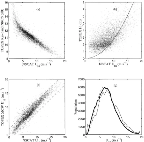
3. The training set—NSCAT and TOPEX
Figure 1 presents TOPEX altimeter parameters versus NSCAT-derived wind speed for the TOPEX/NSCAT collocation dataset. Only one tenth of the total sampling are represented in Figs. 1a–c. Figure 1a shows TOPEX Ku-band soversus NSCAT wind speed. Their relation
appears to be close to linear above 5–6 m s21, while,
with decreasing wind speeds,soincreases rapidly. One
can note thatsoscatter is on the order of 1–2 dB for a
given wind speed. This scatter also increases with de-creasing wind speed. An obvious feature of the large dataset is measurement across a range of ocean wind speeds but note that the population lessens above 15 m s21.
FIG. 1. (a) TOPEX Ku-bandso, (b) TOPEX HS, and (c) TOPEX MCW-derived wind speed—all versus the reference NSCAT 10-m wind speed. (d) Histograms for UNSCAT(thick), UECMWF(dashed), and
UMCW(thin). The model curve in (b) represents fully developed seas
[image:5.612.71.300.70.296.2]for a given NSCAT wind speed using the Sverdup–Munk model.
FIG. 2. Spatial density of TOPEX/NSCAT satellite crossover points used in this study.
observed range of sea-state conditions and HSwind
de-pendence are consistent with past global TOPEX ob-servations (e.g., Callahan et al. 1994). A model curve is superposed on the graph representing HSfor a wind
sea that has reached full development under a given wind (Sverdrup and Munk 1947). Observed HSvalues
falling below this curve likely indicate cases where a wind sea is building. For light to moderate winds HS
data usually exceed this curve indicating that a swell component is common. It follows that idealized fetch-limited wind sea situations are infrequent on the open ocean. This holds except for cases of high wind speeds where swell becomes a much smaller contributor within the total wave height.
Figure 1c presents altimeter wind speed estimated from the operational TOPEX algorithm (Witter and Chelton 1991), showing that wind differences frequently exceed 62 m s21. About 15% of the TOPEX-derived
wind estimates exceed these bounds within the complete TOPEX/NSCAT dataset. Furthermore, a systematic overestimation of wind speed by about 0.5 m s21 is
[image:5.612.122.485.452.606.2]observed over the whole wind speed range. This bias is confirmed by the wind speed histograms presented in Fig. 1d. This same level of bias has also been pointed out in past studies (e.g., Freilich and Challenor 1994). Figure 1d also provides the wind speed histogram for collocated ECMWF wind model data. There is excellent agreement between the NSCAT and ECMWF estima-tion. Note that the global wind distributions show pre-vailing ocean wind speeds fall between 3 and 12 m s21.
This strong weighting of the sampled population to-wards a median value near 7 m s21needs consideration
in wind model developments and validation.
[image:5.612.227.394.648.697.2]FIG. 3. NSCAT and ECMWF wind speed comparisons: (a) bin-averaged relations (dashed) and symmetrical linear regression (solid); (b) standard deviation of the Unscat2Uecmwfwind difference, as a
function of NSCAT wind (dashed) and ECMWF wind (solid).
increased likelihood of high-latitude intersections. This same polar weighting is evident in the TOPEX/ERS and TOPEX/QSCAT data.
Next is an assessment of the chosen reference wind product for model developments—NSCAT’s 10-m wind derived from a 25-km wind vector cell. As noted earlier, scatterometer data are restricted to winds derived using radar incidence angles above 408to ameliorate possible wind speed errors associated with long waves or sea state. For indepth validation of the NSCAT winds and the NSCAT-1 geophysical model function see Freilich and Dunbar (1999) and Wentz and Smith (1999).
Figure 3a presents bin-averaged relations (1 m s21
bin width) and an orthogonal linear regression between the ECMWF model wind and the NSCAT product. As mentioned earlier the model winds have been interpo-lated and are a lower resolution product to begin with. Both products will have substantial rms about a ‘‘true’’ wind measurement as well as possible biases. An or-thogonal linear regression is provided to show results are invariant with choice of regressor. The comparison between the two parameters shows excellent agreement with a slight bias that never exceeds 0.3 m s21 in the
average of one estimate when averaged over binned subsets of the other.
Referencing Fig. 3b one sees that standard deviation (std) of the UNSCAT2UECMWFwind difference as a
func-tion of ECMWF or NSCAT wind speed is about constant at 1.7 m s21for winds less than 10 m s21. For higher
wind speeds the std increases strongly—up to 2.4 m s21
at 16 m s21. This increase is likely associated with the
different resolution cells for NSCAT (25 km) and ECMWF (120 km). This becomes more important for stronger winds because they are likely to be associated with smaller-scale meteorological features.
The cross correlation between significant wave height, altimeter backscatter and surface wind is now addressed. Figure 4 displays a gridding of so versus UNSCAT with color representing the average value for
altimeter-derived HSat a given wind speed ands o. One
can observe a clear dependence of altimeter so upon
HSvariation for a given U10. The relative magnitude of
the change decreases with increasing wind speed. How-ever, the variance is quite strong for common ocean wind speeds, such as the 2-dB range at 6 m s21. Such
a 2-dB range translates to large wind error for the MCW
sowind speed algorithm where wind sensitivity is about
3 m s21dB21at 6 m s21.
It is important to recognize that the pattern that emerges in Fig. 4 is due to the very large amount and global nature of the assembled dataset. Much of the space mapped here represents infrequent events and high latitude observations that might not be seen in smaller and more localized composite datasets (e.g., al-timeter collocations with the NDBC buoy network ob-servations). One can expect such a mapping to gain even better definition with a long-term multiyear data com-pilation where the sampling of sparse regions and in-frequent events increases (e.g., continued collocation between TOPEX/Jason-1 and the SeaWinds sensors).
The observed correlation between altimeter so and HSfor any fixed wind speed confirms, at least in some respects, numerous past studies suggesting sea-state im-pacts on altimeter wind estimations as discussed in our introduction and first noted by Monaldo and Dobson (1989). Cursory inspection of the GEOSAT/NDBC da-taset used for many past sea state impact studies indi-cated little of the variations seen in Fig. 4 and as such, inconclusive findings (cf. Wu 1999) are not surprising. Another means of illustrating the sea-state impact is in terms of the operational altimeter wind product. Fig-ure 5 (left panel) provides that TOPEX estimate versus the coincident ECMWF model wind speed for varied
HSlevels. The TOPEX wind bias is systematically above or below the reference wind for a given HS. NSCAT
wind data (right panel) for the same conditions indicate that the scatterometer wind product shows a negligible relation to HSvariation. These data affirm that the
al-timeter exhibits this mean HSdependence, whereas the
high angle scatterometer winds do not.
We reemphasize that the results shown here depict the average, not instantaneous, globally derived signa-tures. Moreover, significant wave height is the lowest-order moment of the directional wave height spectrum, and HSdoes not necessarily covary with the long wave
slope statistics that correlate more closely withso
mea-surements. Therefore, just as for the backscatter alone, one anticipates no unique pairing ofsoand H
Sthat maps
to a unique U10. Ambiguity is likely to remain due to
the indeterminate ratio of sea versus swell within HS,
the indeterminate direction of the sea versus the swell, unknown fetch and duration, etc. The notion that HSis
a limited surrogate for actual long wave impacts in al-timeter U10 inversion should be kept in mind when
de-veloping a two-parameter (soand H
S) wind speed
al-gorithm for the altimeter.
4. Two-parameter model functions
As discussed, a sea-state impact upon so
pre-FIG. 4. Grid for TOPEXsovs NSCAT wind speed and HS, where color represents the average value for
HS. Bin width : 0.2 m s21, 0.1 dB.
FIG. 5. Symetrical linear regression between (a) Umcwand Uecmwf,
(b) Unscat, and Uecmwfvs ECMWF U10for different SWH classes: 1 m
(dashed line), 3 m (dotted line), 5 m (solid line). The HSrange is
60.5 m about the indicated value.
vailing wind speed inversion for TOPEX still follows the single parameter MCW model:
o
s 5 fMCW(U ).10 (1)
The NSCAT/TOPEX data offers a new opportunity to develop a globally based altimeter wind speed so-lution relevant for operational usage. That is, invert U10
using solely those two products measured by any Ku-band altimeter:
o
U105 f (1s , H ).S (2)
Referring back to Fig. 4 one can see that the three-dimensional representation indicates some nonlinearity, particularly when considering both high and low wind speed regimes. For this reason we choose artificial neu-ral networks to develop the empirical model relating these three parameters, so, H
S, and U10. This choice
assures a robust nonparametric mapping, with one ram-ification being that a derivative sea-state parameter such as pseudowave age (e.g., Glazman and Greysukh 1993) that combines wind speed (or so) with H
S should be
encompassed by this solution.
The overall objective in this nonparametric regression is to generate a globally faithful and continuous rep-resentation of the observed relation between a reference
U10and TOPEX measurements. A most direct inversion
is given by f1[Eq. (2)]. However, from a physical or
sensor perspective one anticipates that Ku-bandso
ob-servations are correlated with the local wind waves (U10)
but also with the long wave roughness and its surrogate,
HS. As such, a more physically relevant (forward) model treats those latter variables as network inputs andsoas
the output:
o
FIG. 6. Correlation of the dependent variable in (a) f2and (b) f1
with variation in HS: y axis depicts the value of the linear correlation coefficient computed at each respective x-axis location.
TABLE2. Coefficients for the f1model.
Parameter Matrix elements
Wx
Wy
Bx
By
P
233.95062
23.93428 0.54012 18.06378
22.28387 0
as01bs0s
211.03394
20.05834 10.40481
20.37228 . . .
aHS1b HHS S
TABLE1. Input and output data scaling coefficients needed for both neural network models.
Parameter a b
s0
HS
U10
20.34336 0.08725 0.10000
0.06909 0.06374 0.02844
TABLE3. Coefficients for the f2model.
Parameter Matrix elements
Wx
Wy
Bx
By
P
243.39541 2.78612 1.18281 7.83459 1.13906
1 U10
aU10 bU10
26.92550 1.22293
23.30096
21.46489 . . .
1 HS
aHS bHS
Wind speed is readily derived from f2by inversion
using a look-up table. These two functions [Eqs. (2) and (3)] will not necessarily provide identical U10values for
identicalsoand H
Sinputs.
This point is deduced from the relatively high cor-relation observed between the radar backscatter and HS
in comparison to the correlation between NSCAT’s wind speed and HS(see Fig. 6). At a given value of its first
input parameter so (U
10), the f1 ( f2) mapping has a
relatively lower (higher) correlation between its output variable U10(s
o) and H
S. The input variables [U10, HS]
for f2are less self-correlated than those for f1. Thus,
the f2mapping is expected to weight the sea-state
pa-rameter more strongly than f1.
Detail for f1and f2model developments are provided
in appendix A. In initial studies (Gourrion et al. 2000) two differing neural techniques were applied to the TO-PEX/NSCAT data. The first approach used a general regression neural network (GRNN) and the second ap-proach used the multilayer perceptron (MLP). That re-port concludes that the two approaches give results that are in close agreement. This paper reports only the MLP solutions as they provide closed-form solutions that are most readily disseminated.
a. Model definition
Given the input pair [so, H
S] or [U10, HS] the
fol-lowing equations and coefficients (Tables 1, 2, and 3) define the analytical neural network solutions f1and f2,
respectively.
The f1 solution provides an altimeter-derived 10-m
neutral-stability wind speed trained to the NSCAT-1 model function output:
Yf12aU10
U105 f15 , (4)
bU10
while f2predicts the normalized radar cross section at
Ku-band and for vertical incidence:
Yf 2 aso
2 o
s 5 f25 . (5)
bso
The variable Y (for either f1or f2) is derived as
T T 2(W Xy 1B )y 21
Y5 [1 1 exp ] , (6)
with X defined as
T T 2(W Px f1B )x 21
X 5[1 1 exp ] . (7)
The subscripts on scaling coefficients (a and b) corre-spond to the appropriate altimeter parameter, boldface variables are vectors, andTdenotes the vector transpose.
Here, P (respectively P ) is the two-row input matrixf1 f2
to the f1( f2) transfer function given by
o f
sf U10
, respectively ,
1 2
HfS1 2
HfSthe;denoting data normalized with the appropriate a and b coefficients. Equations (4) and (5) provide the network outputs once renormalized using these coeffi-cients.
FIG. 7. (a),(b) represent the average over the input data domain for the f1(left) and f2(right) models as derived from TOPEX/NSCAT
[image:9.612.168.527.70.313.2]dataset. (c),(d) represent the overall behavior of the neural network solutions. Curves depict data or model results about three different SWH values: 1 m (circles), 3 m (pluses), and 5 m (squares). The MCW model is overlaid for comparison (thick line).
FIG. 8. Frequency distribution of wind speeds over the entire NSCAT/TOPEX dataset.
FIG. 9. (a) The average of TOPEX HSvalues for a given NSCAT
U10(60.5 m s21) and TOPEXso512.2 (60.2 dB). (right panel)
(b) The average NSCAT U10at differing zonal bands for the fixed
TOPEX data pair [so512.2 (60.2), HS51.7 (60.2)].
attenuating property of the log-sigmoid is what allows us to represent nonlinear input–output relationships within our training and test data.
As described in appendix A, we empirically deter-mined that adequate characterization is obtained with a three-layer MLP network. Model outputs are readily calculated with the simple matrix operations defined in Eqs. (4)–(7).
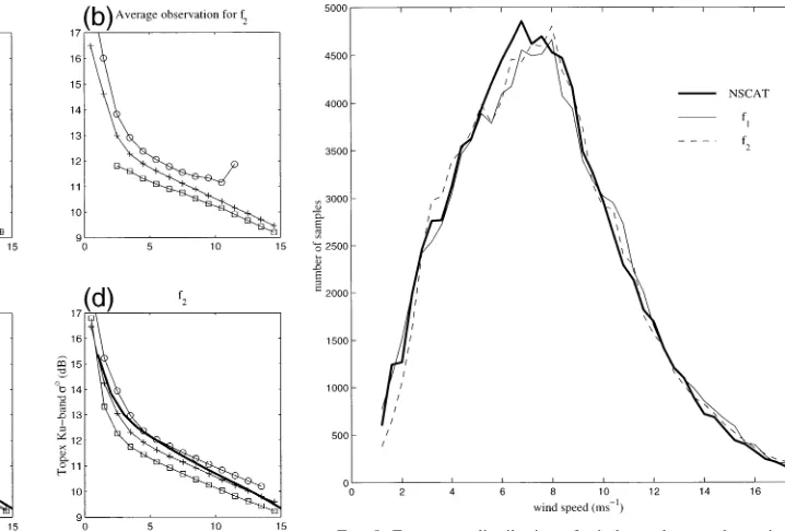
[image:9.612.314.540.548.668.2]b. Model results
Figure 7 illustrates model response versus so and
versus wind speed for three separate HSvalues. Upper
panels depict the average TOPEX/NSCAT observations and are representative of the f1and f2training sets. The
standard TOPEX routine (MCW) is displayed for ref-erence. Both neural models clearly differ from this MCW result. The observations and models also make it clear that the f1 mapping differs substantially from
f2. As already discussed, this may lead to differences
with respect to HSimpacts on wind inversion.
Differ-ences are particularly evident in Fig. 7 at low and high
U10. Overall, it is apparent that the f1model represents
a weaker departure from MCW.
Histograms of NSCAT and model-derived winds are shown in Fig. 8. Wind speed is retrieved from f2using
a look-up table. The histogram bin size here is 1.0 m s21. Agreement between the three products is close, with
the models missing only slightly in the range of 5–7 m s21. Referring back to Fig. 1, one observes that the new
functions appear to improve over MCW.
Finally, recall that multivaluedness within this par-ticular three parameter dataset thwarts efforts to further refine model performance by various methods such as changing the training set makeup, network size, or data limits. That is, given altimeter measurement pairs [so, HS] do not always map to a unique wind speed. This property is partially attributed to the fact that HS is a
limited proxy for the actual long wave conditions dic-tating the relation between so and U
10. Illustration is
provided in Fig. 9, where the left panel shows observed
U10 ranging from 4 to 8 m s21 for fixed values of HS
(1.7 m) andso(12.2 dB). The right-hand panel provides
na-TABLE4. Wind speed error statistics for TOPEX altimeter U10
de-rived using the specified algorithms. Computations are made over the 96 436 samples within the collocated dataset TOPEX/NSCAT where the reference NSCAT wind speed fell between 1 and 17 m s21. Error
trends are the slopesain the linear regression model Uerr5b 1 aX
where X is UNSCATor HS. The separation time between altimeter and
scatterometer estimates is61 h. Altimeter
model Bias
(m s21) Std Rms
% error
.2 m s21
U error trend
HSerror trend B81 MCW FC GG2 Lefe`vre f1 f2 0.36 0.61 0.02 0.04 0.28 0.04 0.01 1.16 1.19 1.22 1.07 1.44 1.05 1.10 1.22 1.34 1.22 1.07 1.47 1.05 1.10 9 12 7 5 15 5 6 20.22 0.03 0.03 20.06 20.28 0.00 20.02 20.04 0.48 0.48 0.17 0.17 0.20 20.06
ture. This plot shows systematic U10 variance versus
latitude for the specified [so, H
S] pair. To first order,
this latitudinal dependence indicates some regional change in the long wave climate. Toward the poles there is typically a larger ratio between swell and wind waves within the total sea state. Wind speed is systematically 0.6 m s21lower than at midlatitudes. Regardless of the
source, a multivalued behavior manifests itself in em-pirical model training as a fundamental error source that the network cannot resolve without additional infor-mation. This is true for both f1and f2mappings. The
latitudinal dependence evident in Fig. 9 also suggests that the improved two-parameter altimeter wind models will still exhibit residuals in regional or seasonal eval-uations. Further work on these points is warranted but deemed beyond the scope of the present effort.
5. Wind speed model intercomparison
This section uses the total TOPEX/NSCAT data to compare model-derived results with previously pub-lished altimeter wind speed routines. A following sec-tion documents addisec-tional independent validasec-tion. A key study objective is to provide wind estimates with im-proved overall statistical performance when applied to global open-ocean observations. Past efforts have em-phasized that the measure for algorithm accuracy should not solely be the global wind speed error (cf. Glazman and Greysukh 1993). The large amount of data in our training and validation datasets permits detailed wind error evaluation. This includes the ability to assess error at light, moderate and high wind speeds, as well as the identification of residual correlation with the reference wind speed and/or HS. Evaluation criteria values both
bias and rms minimization. Due to operational and cli-mate study considerations, a continuous function is also desired. Moreover, estimates should produce a faithful global wind speed histogram.
There are many published altimeter wind speed mod-els that use only the Ku-bandso. A review is found in
Chelton et al. (2001). Here, the choice of single-param-eter algorithms for intercomparison is limited to Brown et al. (1981), Witter and Chelton (1991), and Freilich and Challenor (1994). These are noted as B81, MCW, and FC, respectively, in the text to follow. The conten-tion is that these models encompass most other varia-tions—B81 represents a buoy-tuned discontinuous (three branch) function that has often produced the low-est overall rms, whereas MCW and FC represent smoother, statistically derived functions that are well-validated and robust.
Two wind speed models that utilize both the Ku-band
soand H
Sare also assessed. Lefe`vre et al. (1994)
pro-vides a closed-form parametric solution as a function of the two altimeter inputs based on comparison between TOPEX and wind model (ARPEGE, the Meteo-France atmospheric model) data. Glazman and Greysukh (1993, GG2 hereafter) developed a classification approach
where wind speed is estimated using one of two dis-tinctly separate single parameter (so → U
10) models.
This work was based on comparisons between the GEO-SAT altimeter and buoy-derived wind and wave mea-surements. For operational inversion, the classification relies on altimeter HSand soestimates. The two GG2
wind models are rooted in the concept of pseudowave age, z[.f (HS/U2)], where the first model is for
‘‘young’’ or fetch-limited wind wave conditions and the second covers all other situations (i.e., covering fully developed seas and the ubiquitous mixed seas). As noted in GG2, the classification is inherently discontinuous and leads to bimodality in the output U10 distribution.
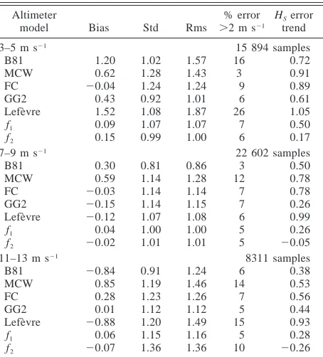
Table 4 presents wind speed differences between the altimeter and scatterometer for the commonly cited case where statistics are computed over all wind values. Computations for each altimeter algorithm are included. The reference (NSCAT) U10range used here is 1–17 m
s21. The limits encompass the range of conditions over
which most of the models were developed. Note that, where applicable, TOPEXsovalues are adjusted down
by 0.63 dB before use in GEOSAT-era routines (see Callahan et al. 1994).
The wind speed difference Uerris defined as altimeter reference
Uerr5 U10 2 U10 , (8)
where the reference is NSCAT in this case and the neu-tral stability wind speed is given in meters per second. Wind error standard deviation is simply
2 2 1/ 2 2 2 1/ 2
std5(^Uerr& 2 ^Uerr& ) 5 (rms 2bias ) . (9) This factor provides bias-independent rms assessment and is of some value in the following discussion where small differences become significant.
TABLE5. Results follow the same format as table 4, but estimates are now localized to three separate wind speeds (4, 8, and 12 m s21)
as indicated. Altimeter
model Bias Std Rms
% error
.2 m s21
HSerror trend
3–5 m s21 15 894 samples
B81 MCW FC GG2 Lefe`vre f1 f2 1.20 0.62 20.04 0.43 1.52 0.09 0.15 1.02 1.28 1.24 0.92 1.08 1.07 0.99 1.57 1.43 1.24 1.01 1.87 1.07 1.00 16 3 9 6 26 7 6 0.72 0.91 0.89 0.61 1.05 0.50 0.17
7–9 m s21 22 602 samples
B81 MCW FC GG2 Lefe`vre f1 f2 0.30 0.59 20.03 20.15 20.12 0.04 20.02 0.81 1.14 1.14 1.14 1.07 1.00 1.01 0.86 1.28 1.14 1.15 1.08 1.00 1.01 3 12 7 7 6 5 5 0.50 0.78 0.78 0.26 0.99 0.26 20.05
11–13 m s21 8311 samples
B81 MCW FC GG2 Lefe`vre f1 f2 20.84 0.85 0.28 0.01 20.88 0.06 20.07 0.91 1.19 1.23 1.12 1.20 1.15 1.36 1.24 1.46 1.26 1.12 1.49 1.16 1.36 6 14 7 5 15 5 10 0.38 0.53 0.56 0.44 0.93 0.28 20.26
Hwang et al. 1998). The largest temporal separation here is one hour. Total sample population is more than 96 000, thus parameter noise levels are negligible.
The overall bias for any altimeter routine is well be-low 1 m s21with only MCW output showing a value
above 0.5. Slopes computed for the linear trend of Uerr
versus wind speed are provided as some indication of bias variability with wind speed. It is clear that B81 and Lefevre model bias trends are much higher than for the other routines. The most commonly reported assessment parameter, global rms, shows values spanning from 1.05 to 1.47. The Lefevre algorithm exhibits the highest error. The single parameter models (B81, MCW, and FC) ex-hibit similar rms and std estimates (1.2) while the 3 two-parameter algorithms (GG2, f1, f2) are below 1.10.
Table 4 also provides a column representing the wind error slope versus HSfor consistency with Freilich and
Challenor (1994). But this parameter is of questionable meaning when taken over all wind speeds and a much clearer picture emerges when viewing that error trend for specific U10 levels as shown in Table 5. This table
summarizes local error estimates near 4, 8, and 12 m s21that provide measures at the most populated
mod-erate wind region, and for low and high wind levels where there is still a substantial data population. Con-tinuous detail versus the reference U10 is provided in
Fig. 10. The panels show wind error bias, standard de-viation, and rms along with the linear regression cor-relation coefficient (R) for wind error versus HS.
Residual statistics versus wind speed are not typically cited in altimeter wind studies, often due to the limited
data samples and hence high uncertainty. But this in-formation helps to ascertain small but measurable al-gorithm differences. Referring to Table 5 and Fig. 10, it becomes evident that overall B81 statistics of Table 4 can be misleading. The figure shows that B81 has the lowest rms error in the range of 7–9 m s21. But highest
rms levels then occur for B81 at low and high winds in step with the bias magnitude. B81 also presents lower wind error standard deviation than the other single pa-rameter algorithms, again related to wind-dependent bias. B81 bias variation relates directly to the20.22 m s21 error trend of Table 4 and seems consistent with
Freilich and Challenor (1994) who noted that the chosen three-branch form of the Brown model leads directly to these characteristics. All indications are that B81 is a weaker choice for wind inversion than, for example, MCW or FC.
The MCW statistics exhibit constancy (bias, std, HS
-related residual) versus U10, but a constant positive bias
of about 0.5 to 0.6 m s21 produces a systematically
elevated rms. This bias agrees with other studies (e.g., Glazman and Greyzukh 1993; Freilich and Challenor 1994). The FC model presents a lower bias as well as stable rms and bias variation over all winds. In fact, we conclude that FC is nearly equivalent to MCW aside from this 0.5 m s21 constant. For example, H
S
corre-lation for MCW and FC in Fig. 10 is almost identical. Perhaps the most notable observation regarding single parameter models is the measurable correlation between wind error and the altimeter-derived HS for any wind
speed. The error slope (and linear regression correlation coefficient) is strongest in the range 4–9 m s21 with
values of 0.8–0.9. Correlation decreases slightly for the lowest and highest U10and reaches a minimum at
high-est winds.
Tables 4 and 5 and Fig. 10 show that the two input algorithms provide low bias levels and consistently low-er standard deviations aside from Lefe`vre et al. (1994). Considering all factors, it is evident that the Lefevre model performs poorly and this algorithm will not be discussed further.
Data indicate that the GG2 model leads to wind error statistics that often match the low levels obtained with the neural network solutions. But the bias is somewhat erratic versus U10. One feature of this model is the abrupt
lowering of the HSerror trend for moderate wind speeds
of 7–9 m s21seen in Fig. 10. Aside from this region,
the HSimpact (error trend or correlation) is nearly
iden-tical to the single parameter algorithms. This localized use of the HSinput is a feature of the two-class scheme
used in that algorithm combined with the large range of possible [so, H
S] combinations within this moderate
wind range. Basically, the GG2 leads to a bimodal wind histogram (not shown) due to its discontinuous nature, much as for B81.
As alluded to earlier, the HSerror trend for a given U10will, by design, be significantly reduced in the neural
[image:11.612.72.299.100.351.2]FIG. 10. Altimeter wind speed error statistics for the cited algorithms as a function of NSCAT U10: (a)
bias, (c) standard deviation, (b) SWH correlation with wind error, and (d) rms. Calculations are made over 2 m s21bins.
5 and Fig. 10 clearly indicate that the f2routine strongly
attenuates the HSresidual (to less than 0.1 m s21m21
while MCW and FC were generally higher than 0.6 m s21 m21). The f
1 model provides a reduction but not
removal of this correlation. Recall that these two al-gorithms carry different weighting of HS due to their
alternate training. Both neural solutions provide a very small and stable bias across the complete wind speed range. The rms for the two solutions is nearly identical up to 10 m s21and at that point the f
2begins to increase
substantially with increasing wind speed. This increase is partially related to the aforementioned multivalued-ness that the neural network encounters when attempting to optimize the [U10, HS]→somapping over both
erate and high wind speeds. The forward network mod-el, f2, upon inversion to wind speed, can actually lead
to a negative correlation with HSat high winds as seen
in Table 5. Thus while f2best removes the HS
depen-dence and may represent a better physically based model for Ku-bandsoas a function of H
S(surrogate for wave
climate), the model is not optimal for point-to-point U10
inversion. This observation is strong evidence in support of the idea that HSdoes not directly describe true long
wave conditions that cloud the mapping between U10
andso.
Considering all algorithms and observations includ-ing their bias, functional continuity and rms error min-imization, it appears that f1 provides the best overall
altimeter wind speed model. The improvement (relative to the operational MCW model) is on the order of 10%– 15% in terms of the global or local reduction in the wind error standard deviation or rms. In an absolute sense, the new routine appears to lower the rms error by 0.1–0.2 m s21. Improvements are negligible for the
high winds above 12–14 m s21. The bias is minimized
to less than 0.1 m s21over all wind speeds. These
TABLE6. Altimeter Uerrstatistics as for Table 4, but where the reference U10now changes with each row as indicated. The three TOPEX/
ECMWF subsets come respectively from the TOPEX/NSCAT, TOPEX/QSCAT, and TOPEX/ERS compilations as discussed in section 2. Separation times for altimeter comparisons with scatterometer and buoy observations is630 min in all cases. Computations are made over the reference wind range of 1 to 17 m s21. The slope of the error trend with HS(see Table 4) is given asa
Hs. Dataset Time period Extent (month) No. of samples FC
Bias Std aHS
f1
Bias Std aHS
TOPEX/NSCAT TOPEX/QSCAT ERS/NSCAT TOPEX/ERS 1996–97 1999–00 1996–97 1995–97 9 12 9 24 48 331 88 324 129 701 55 765 0.02 20.48 20.70 20.07 1.16 1.18 1.02 1.08 0.49 0.44 0.47 0.27 0.05 20.53 20.56 20.08 0.99 0.97 0.87 1.01 0.20 0.15 0.16 20.03 TOPEX/ECMWF1 TOPEX/ECMWF2 TOPEX/ECMWF3 TOPEX/BUOY 1996–97 1999–00 1995–97 1992–98 9 12 24 75 231 102 312 102 208 518 4380 20.24 0.03 20.06 20.32 1.84 1.46 1.64 1.45 0.38 0.37 0.25 0.56 20.20 0.03 20.05 20.132 1.77 1.43 1.56 1.33 0.14 0.08 0.01 0.26
TABLE7. Results follow the same format as table 6, but estimates are now localized to three separate wind speeds (4, 8, and 12 m s21)
as indicated.
Dataset
FC Bias Std aHS
f1
Bias Std aHS
3–5 m s21
TOPEX/NSCAT TOPEX/QSCAT ERS/NSCAT TOPEX/ERS TOPEX/ECMWF1 TOPEX/ECMWF2 TOPEX/ECMWF3 TOPEX/BUOY 20.03 20.65 20.92 0.08 20.01 20.01 0.05 20.34 1.23 1.07 0.86 1.12 1.85 1.46 1.63 1.49 0.92 0.70 0.53 0.79 0.93 0.66 0.81 0.80 0.10 20.50 20.72 0.21 0.13 0.18 0.19 20.03 1.05 0.89 0.76 0.94 1.83 1.40 1.57 1.43 0.52 0.39 0.29 0.38 0.59 0.28 0.44 0.51 7–9 m s21
TOPEX/NSCAT TOPEX/QSCAT ERS/NSCAT TOPEX/ERS TOPEX/ECMWF1 TOPEX/ECMWF2 TOPEX/ECMWF3 TOPEX/BUOY 20.07 20.47 20.77 20.11 20.34 20.04 20.04 20.46 1.09 1.10 0.89 0.91 1.72 1.38 1.52 1.35 0.78 0.72 0.67 0.54 0.94 0.66 0.76 0.86 0.03 20.38 20.53 20.09 20.27 0.02 20.01 20.18 0.95 0.96 0.79 0.84 1.68 1.34 1.47 1.19 0.27 0.17 0.11 20.03 0.47 0.14 0.25 0.34 11–13 m s21
TOPEX/NSCAT TOPEX/QSCAT ERS/NSCAT TOPEX/ERS TOPEX/ERS2 TOPEX/ECMWF1 TOPEX/ECMWF2 TOPEX/ECMWF3 TOPEX/BUOY 0.31 20.49 20.29 20.20 20.14 20.39 0.13 20.21 20.08 1.14 1.14 1.10 0.97 0.76 1.78 1.53 1.52 1.59 0.57 0.54 0.48 0.44 0.39 0.68 0.59 0.51 0.88 0.10 20.70 20.40 20.43 20.38 20.58 20.14 20.47 20.05 1.05 1.04 1.01 0.90 0.68 1.69 1.50 1.50 1.41 0.30 0.20 0.18 0.12 0.05 0.45 0.29 0.20 0.63
of independence and confidence for these conclusions within the assumption that NSCAT winds represent a valid U10N reference. Attention is now given to
addi-tional algorithm validation using the numerous inde-pendent data products discussed earlier.
6. Further model validation
Model intercomparisons presented above suggest that the two-input altimeter algorithm, f1, provides the best
performance. The model is now evaluated against the
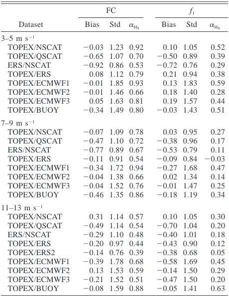
seven additional collocation datasets detailed earlier. These sets include independent altimeter (ERS-2) mea-surements as well as reference wind speed estimates from C- and Ku-band scatterometers, the ECMWF mod-el, and a large open-ocean buoy compilation. The varied reference winds encompass most sources used in past altimeter studies and they each present differing spatial sampling, TOPEX time period, and scattering or model physics. The main goal here is to determine if the al-gorithm provides consistently improved results across these varied sources. Expanded detail in support of the following findings can be found in Gourrion et al. (2000).
Initial altimeter algorithm assessment against these data indicates that relative differences amongst the al-gorithms discussed in the previous section (e.g., f1
per-formance vs f2) remain consistent with the TOPEX/
NSCAT findings. Therefore presentation is condensed to compare and contrast the preferred single and two-parameter routines: FC and f1. As mentioned earlier,
FC is essentially the operational MCW routine without a 0.5 m s21overall bias.
Altimeter wind error statistics are presented in Tables 6 and 7. Sample population and time period covered are listed in Table 6. Note that the buoy dataset covers the longest time period, yet contains the fewest points.
Look first to U10 bias values. It is evident that both
the FC and f1models provide biases that fall below 0.5
m s21for all TOPEX cases. Given that the combined
periods span from 1992 to 2000, this is, first of all, an indication of long-term stability for the satellite’s so
calibration. For reference, asochange of 0.1 dB
cor-responds to roughly 0.3 m s21 in wind speed for the
altimeter. The ERS-2 altimeter (ERS/NSCAT in the ta-bles) exhibits a consistent 0.5 to 0.9 m s21bias below
TOPEX for both the FC and f1models. This translates
to a small10.2 to 0.3 dB sobias range between the ERS-2 altimeter and TOPEX. Returning to the TOPEX
table entries, the bias differences between FC and f1,
for any given dataset in Tables 6 and 7, are very small; in almost all cases less than 0.1 m s21. Agreement
[image:13.612.70.300.411.708.2]pro-posed f1implies that a switch to use of the latter model
should be seamless.
One possible outlier with respect to the altimeter wind speed bias (for both FC and f1) comes in the QSCAT
comparison. Here the TOPEX bias is consistently below other sets by about 0.5 m s21. Recall that QSCAT is a
Ku-band scatterometer but differs from NSCAT in sev-eral aspects, the most important being the scatterometer model function. We noted in section 2 that the NSCAT-1 model function was purported to be 0.3 m s21too low
and that the QSCAT-1 model is without this bias. Rais-ing the NSCAT-1 model by 0.3 m s21would bring
PEX closer to QSCAT but also, consequently, bias TO-PEX above most other table entries. The weight of the other data presented here, including possible time-de-pendent sensor and model bias variations, is not ade-quate to accept or dismiss bias adjustments at this small level. Averaging the bias values over all TOPEX entries of Table 7, one concludes that the absolute wind speed bias level is below 0.3 m s21 for both f
1 and FC
al-gorithms.
Reduction in the error variation versus HSis the prime
indicator of a difference between the FC and f1
algo-rithms. The reduction is evident for all aHs entries in Table 7. This is consistent with the results of the pre-vious section and with the goal of attenuating long-wave impact on the altimeter wind speed. Some disparity be-tween particular reference sets is evident, but the re-duction is not. The values of FCaHsrange from 0.6 to 0.9 and the f1model lowers these levels on average by
factors of 1.8, 3.5, and 2.4 at 4, 8, and 12 m s21,
re-spectively. Thus, regardless of possible sampling or product disparities, the sea state–related impact is al-ways measurably decreased in a global average sense. Similar results hold for those wind levels not shown, consistent with Fig. 10.
Finally, the rms wind error is assessed using the stan-dard deviation to directly compare (without bias) FC and f1results. Reference winds lead to some clear
dif-ferences here for the TOPEX data sets. Scatterometer-based comparisons using NSCAT, QSCAT, and ERS, all provide the lowest std levels, generally between 0.9 and 1.2 m s21. As before, f
1output reduces the std by 10%
to 15% overall and at the noted wind speeds. The TO-PEX–ECMWF comparisons show std levels of 1.5–1.8, an increase of 30%–45% over results obtained using the scatterometers. This rise is consistent with the expected increase in intercomparison noise due to ECMWF’s in-herently larger time and space averaging as predicted by Freilich and Dunbar (1993). Moreover, the std re-duction obtained using f1is not so dramatic, only 3%–
5%. So while the HS dependence (a) is clearly
atten-uated in the ECMWF comparisons using the f1
algo-rithm, the elevated intercomparison noise tends to mask the precision gained. Note that the ERS/NSCAT com-parison usually indicates the lowest std levels, and these values are also comparable to those of the TOPEX/ERS computations. The common factor between these two
datasets, not found in the others, is the use of a 50-km scatterometer wind vector cell. The lower std levels for these table entries may be associated with a possible reduction in the scatterometer’s inherent wind estimate noise. Regardless, the nominal 10%–15% reduction in std is still found when using f1 in lieu of the FC
al-gorithm.
a. Buoy comparison
Comparison between TOPEX-derived wind speed and buoy measurements represents our only in situ val-idation. For this reason, greater detail is presented here. Further information on this particular data set can be found in Gommenginger et al. (2002). Findings to fol-low were also affirmed by comparing GEOSAT altim-eter data to NDBC buoy observations in Gourrion et al. (2000). Comparison statistics are listed in Tables 6 and 7. The results are generally consistent with the findings above. Note however that std values are now of the order of 1.4 m s21instead of the 1.0 m s21levels found
for the altimeter/scatterometer validation datasets. This may be attributed to differences in measurement tech-niques, sampling methods and/or in the time–space col-loction criteria. The std and residual HStrend (aHs)
dis-play a reduction between the one- and two-parameter algorithms, which is consistent with previous validation results. In this case, the improvement in the overall std with the additional parameterization on HSis of the order
of 10%.
Figure 11 presents statistics versus buoy wind speed over the range of 1–17 m s21 calculated in 2 m s21
-wide wind bins incremented by 0.5 m s21. Display
for-mat follows Fig. 10 and results are shown for four al-timeter model functions as indicated. Comparison of Figs. 11 and 10 suggests the altimeter wind error is nearly invariant between these two reference wind prod-ucts for wind speeds above 4–5 m s21. As before, one
sees the FC and MCW models track each other aside from a;0.5 m s21bias. GG2 compares well with the
f1 results in all aspects. These two input models once
again outperform the single parameter mapping. In Fig. 11 and Tables 6 and 7 the f1model returns the smallest
and most stable wind error bias over the full wind speed range, with retrieved winds only slightly underestimated (by 0.2 m s21) at intermediate wind speeds. The std for
GG2 is lowest of all models at low wind speed, although the neural network-derived model is alone in achieving a near-zero bias. Here again we observe that the two-parameter models reduce, but do not eliminate, the re-sidual dependence on HS.
mod-FIG. 11. Altimeter wind error statistics using buoy measurements as the reference wind. Computations and data display follow those for Fig. 10.
FIG. 12. Frequency distributions of wind speed retrieved with (a) MCW and (b) f1along with the buoy-derived result. Bin size is 1.5
m s21.
el, as this is the model currently used for operational wind speed retrieval on TOPEX and ERS altimeters.
The retrieved wind speed histograms are compared to the buoy result in Fig. 12. Visual improvement is evident for f1with respect to MCW. The goodness of
fit is estimated via the computed correlation between
the buoy and model wind speed histograms. One finds a correlation of 0.989 for MCW and 0.994 for f1. The
improved fit is most noticeable at intermediate to high wind speeds (U10 . 8 m s21). Consequently, the
two-parameter f1model is expected to return more accurate
global wind fields than the current operational MCW algorithm.
b. Residual sea-state effects
The availability of in situ wave period measurements within the collocated TOPEX/buoy dataset permits fur-ther investigation of the effect of sea state on altimeter retrieved wind speed. From this dataset a dependence of altimeter wind speed on wave age has been reported (Gommenginger et al. 2002) and MCW winds shown to systematically underestimate winds in underdevel-oped sea conditions (wave age,1.5). Here we assess if wave age dependence is ameliorated by the param-eterization with HSin the f1model. Figure 13 represents
FIG. 13. Residual dependence on buoy-derived wave age (z) ob-served in the retrieved wind error calculated with (a) MCW and with (b) f1.
f1 against the buoy-derived wave age calculated from
the peak wave period, Tp, as z 5gTp(2pU10)2 1. A
de-pendence of the wind error on wave age is clearly ob-served for young seas (z ,1) for both altimeter wind speed algorithms. No residual dependence on wave age is observed for either model for wave age greater than 1.5.
The residual wave age dependence for young seas is quantified with the linear regression coefficient of Uerr
against z calculated for z , 1.0. We find that the pa-rameterization with HS used in the f1 model yields a
marginal reduction in the wave age trend, from 4.0 for MCW to 3.5 m s21per unit of wave age for f
1. However,
the dependence of altimeter wind speeds on wave age in underdeveloped sea conditions certainly remains. Thus the addition of HSinto the algorithm falls far short
of correcting the known underestimation associated with
young seas. It is again notable that only 7% of the total TOPEX/buoy samples over this period of 1992–98 have
z ,1.0. This fraction is consistent with the global ob-servations (see Fig. 1) discussed earlier.
7. Summary
This study defines and validates a two-input altimeter wind speed algorithm applicable for operational use, where a Ku-band altimeter’s coincidentsoand H
S
es-timates are utilized in the point-to-point inversion. An analytical formulation (termed f1) is prescribed with
nine coefficients as detailed in section 4. Motivation comes from the new capability to assemble large, glob-ally distributed and high fidelity model training sets composed of coincident satellite altimeter and scatter-ometer crossovers. The dataset chosen for model train-ing and subsequent validation is a 96 000 sample com-pilation of TOPEX and NSCAT crossings. Limiting NSCAT usage to only higher incidence angle retrievals strengthens our assumption that the scatterometer wind product is itself free of sea-state impacts. Subsequent validations using buoy and ECMWF winds provide fur-ther support.
The empirical development is focused to define an improved and robust wind inversion that incorporates
HSinto the solution. This routine should be applicable for all Ku-band altimeters such as those aboard the ERS, ENVISAT, GFO, and Jason-1 platforms. f1
intercom-parison to past altimeter models and numerous inde-pendent validations demonstrates modest, but measur-able, success in improving upon the current operational MCW model. These independent data sources include an extensive buoy compilation, the ERS scatterometer, the SeaWinds scatterometer, and the ECMWF model. The f1inversion ([so, HS]→[U10N]) delivers an overall
rms improvement of 10–15%, 0.1 to 0.2 m s21in
ab-solute terms. The domain for model application covers all values of HSand wind speeds ranging from 1 to 20
m s21. Error statistics were evaluated over the range of
1–17 m s21. Wind speed bias is below 0.3 m s21
through-out this range. Improvement in rms error is significant up to winds of about 12 m s21and equivalent to MCW
above this point. The weighting of HSwithin the model
becomes negligible at these high wind levels. While wind speeds above 20 m s21 are infrequent, a slight
modification of f1 that aligns the altimeter inversion
with that predicted by the QSCAT-1 model function is proposed in appendix B. Statistically, the GG2 algo-rithm provides similar improvement, but we recall that this classification scheme leads to point-to-point esti-mate discontinuities and a bi-modal wind speed distri-bution. TOPEX wind speed histograms, derived using
f1, provide marked improvement over the MCW result