Multi issue negotiation under time constraints

(1)

Multi-Issue Negotiation Under Time Constraints

Shaheen S. Fatima

Department of Computer

Science University of Liverpool Liverpool L69 7ZF U.K.

Michael Wooldridge

Department of Computer

Science University of Liverpool Liverpool L69 7ZF U.K.

Nicholas R.Jennings

Department of Electronics and

Computer Science University of Southampton Southampton SO17 1BJ U.K.

ABSTRACT

This paper presents a new model for multi-issue negotiation un-der time constraints in an incomplete information setting. In this model the order in which issues are bargained over and agreements are reached is determined endogenously as part of the bargaining equilibrium. We show that the sequential implementation of the equilibrium agreement gives a better outcome than a simultaneous implementation when agents have like, as well as conflicting, time preferences. We also show that the equilibrium solution possesses the properties of uniqueness and symmetry, although it is not al-ways Pareto-optimal.

Categories and Subject Descriptors

I.2.11 [Distributed Artificial Intelligence]: Multiagent Systems; K.4.4 [Computers and Society]: Electronic Commerce

General Terms

Algorithms, Design

Keywords

Negotiation, game theory, agendas

1. INTRODUCTION

Agent mediated negotiation has received considerable attention in thefield of electronic commerce [14, 9, 7]. In many of the appli-cations that are conceived in this domain it is important that the agents should not only bargain over the price of a product, but also take into account aspects like the delivery time, quality, payment methods, and other product specific properties. In such multi-issue negotiations, the agents should be able to negotiate outcomes that are mutually beneficial for both parties [11]. However the com-plexity of the bargaining problem increases rapidly as the number of issues increases. Given this increase in complexity, there is a need to develop software agents that can operate effectively in such circumstances. To this end, this paper reports on the development of a new model for multi-issue negotiation between two agents.

Permission to make digital or hard copies of all or part of this work for personal or classroom use is granted without fee provided that copies are not made or distributed for profit or commercial advantage and that copies bear this notice and the full citation on thefirst page. To copy otherwise, to republish, to post on servers or to redistribute to lists, requires prior specific permission and/or a fee.

AAMAS’02, July 15-19, Bologna, Italy

In such bilateral multi-issue negotiations, one approach is to bun-dle all the issues and discuss them simultaneously. This allows the players to exploit trade-offs among different issues, but requires complex computations to be performed [11]. The other approach — which is computationally simpler — is to negotiate the issues sequentially. Although issue-by-issue negotiation minimizes the complexity of the negotiation procedure, an important question that arises is the order in which the issues are bargained. This ordering is called the negotiation agenda. Moreover, one of the factors that determines the outcome of negotiation is this agenda [4]. To this end, there are two ways of incorporating agendas in the negotia-tion model. One is to fix the agenda exogenously as part of the negotiation procedure [4]. The other way, which is moreflexible, is to allow the bargainers to decide which issue they will negotiate next during the process of negotiation. This is called an endoge-nous agenda [5]. Against this background, this paper presents a multi-issue negotiation model with anendogenous agenda.

To provide a setting for our negotiation model, we consider the case in which negotiation needs to be completed by a specified time (which may be different for the different parties). Apart from the agents’ respective deadlines, the time at which agreement is reached can effect the agents in different ways. An agent can gain utility with time, and have the incentive to reach a late agreement (within the bounds of its deadline). In such a case it is said to be a strong (patient) player. The other possibility is that it can lose util-ity with time and have the incentive to reach an early agreement. It is then said to be a weak (impatient) player. As we will show, this disposition and the actual deadline itself strongly influence the negotiation outcome. Other parameters that effect the outcome in-clude the agents’strategies, their utilities and their reservation lim-its. However, in most practical cases agents do not have complete information on all of these parameters. Thus in this work we focus on bilateral negotiation between agents withtime constraintsand

incomplete information.

(2)

tation scheme. Moreover, we show that the sequential implemen-tation of the equilibrium agreement results in an outcome that is no worse than the outcome for the simultaneous implementation, both when agents have like as well as conflicting time preferences. Finally, we study the properties of the equilibrium solution.

This work extends the state of the art by presenting a more re-alistic negotiation model that captures the following three aspects of many real life bargaining situations. Firstly, it is a model for negotiating multiple issues. Secondly, it takes the time constraints of bargainers into consideration. Thirdly it allows agents to have incomplete information about each other.

In section 2 wefirst give an overview of the single-issue negotia-tion model of [3] and then prove that the mutual strategic behavior of agents where both use their respective optimal strategies results in equilibrium. In section 3 we extend this model to allow multi-issue negotiation and study the properties of the equilibrium solu-tion. Section 4 discusses related work. Finally section 5 gives the conclusions.

2. SINGLE-ISSUE NEGOTIATION MODEL

In this section wefirst provide an overview of the single issue ne-gotiation model and a brief description of the optimal strategies as determined in [3]. Due to lack of space, we describe the optimal strategy determination for one specific negotiation scenario. We then prove that the optimal strategy profiles form sequential equi-librium points.

2.1 The Negotiation Protocol

This is basically an alternating offers protocol. Let denote the buyer,the seller and let [

] denote the range of

val-ues for price that are acceptable to agent, where . A

value for price that is acceptable to both and, i.e., the zone of

agreement, is the interval [

]. (

) is the

price-surplus. denotes agent’s deadline. Let

denote the

price offered by agent at time. Negotiation starts when thefirst

offer is made by an agent. When an agent, say, receives an offer

from agent at time, i.e.,

, it rates the offer using its utility

function

. If the value of

for

at time

is greater than

the value of the counter-offer agentis ready to send at time

, i.e.,

¼ with

then agentaccepts. Otherwise a counter-offer is

made. Thus the action A that agenttakes at timeis defined as:

if if

¼

otherwise

2.2 Counter-offer generation

Since both agents have a deadline, we assume that they use a time dependent tactic (e.g. linear (L), Boulware (B) or Conceder (C)) [2] for generating the offers. In these tactics, the predominant factor used to decide which value to offer next is time. The tactics vary

the value of price depending on the remaining negotiation time, modeled as the above defined constant . The initial offer is a

point in the interval [ ,

]. The constant

multiplied

by the size of interval determines the price to be offered in thefirst proposal by agent(as per [2]). The offer made by agentto agent

at time( ) is modeled as a function depending on

time as follows:

for

for.

Price

Time Pb_max

min

O2 O1

Ps

[image:2.612.333.539.7.140.2]

T

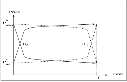
Figure 1: Negotiation outcome for Boulware and Conceder functions

A wide range of time dependent functions can be defined by vary-ing the way in which is computed (see [2] for more details).

However, functions must ensure that ,

and . That is, the offer will always be between the

range

, at the beginning it will give the initial

con-stant and when the deadline is reached it will offer the reservation value. Function is defined as follows:

½

These families of negotiation decision functions (NDF) represent an infinite number of possible tactics, one for each value of .

However, depending on the value of , two extreme sets show

clearly different patterns of behaviour.

1. Boulware[11]. For this tacticand close to zero. The

initial offer is maintained till time is almost exhausted, when the agent concedes up to its reservtion value.

2. Conceder [10]. For this tactic is high. The agent goes

to its reservation value very quickly and maintains the same offer till the deadline. Finally whenprice is increased

linearly.

The value of a counter offer depends on the initial price (IP) at which the agent starts negotiation, thefinal price (FP) beyond which the agent does not concede,and . A vector V of these four

variables, i.e., V = [IP, FP, ,] forms the agent’sstrategy. Let

and . Thenegotiation outcome

is an element of, where the pair () denotes theprice

andtimeat which agreement is reached anddenotes the conflict

outcome.

For example, when ’s strategy is defined as

and ’s strategy is defined as

, the outcome

( ) that results is shown infigure 1. As shown in the figure,

agreement is reached at a price

- and

at a time close to T. Similarly when the NDF in both strategies is replaced with C, then agreement (

) is reached at the same price

but towards the beginning of negotiation.

2.3 Agents’ information state

Each agent has a reservation limit, a deadline, a utility function and a strategy. Thus the buyer and seller each have four parameters denoted

and

respectively.

(3)

The information state of an agent is the information it has

about the negotiation parameters. An agent’s own parameters are known to it, but the information it has about the opponent is not complete.

and

are taken as:

and

where ,

,

and

are the information about ’s own pa-rameters and

and

are its beliefs about

. Similarly, ,

,

and

are

’s own parameters and and

are its

be-liefs about . and

are two lotteries that denote ’s beliefs

about’s deadline and reservation price, where

such that

and

such that

.

Similarly and

are two lotteries that denote

’s beliefs about

’s deadline and reservation price, where

such that

and

such that

.

Thus agents have uncertain information about each other’s dead-line and reservation price. However, the agents do not know their opponent’s utility function or strategy.

Agents’ utilities are defined with the following two von Neumann-Morgenstern utility functions [6] that incorporate the effect of time discounting.

, where and

are

uni-dimensional utility functions. Here, preferences for attribute ,

given the other attribute, do not depend on the level of.

is defined as:

for the buyer

for the seller

is defined as

Æ , where

Æ

is the discounting factor.

Thus when Æ the agent is patient and gains utility with time

and when Æ the agent is impatient and loses utility with

time. Note that the agents may have different discounting factors. Agents are said to have similar time preferences if both gain on time or both lose on time. Otherwise they have conflicting time preferences. Each agent’s information is itsprivateinformation that is not known to the opponent.

2.4 Optimal strategies

We describe how optimal strategies are obtained for players that are von Neumann-Morgenstern expected utility maximizers. Since utility is a function of price and time, these strategies optimize both. The discussion is from the perspective of the buyer (although the same analysis can be taken from the perspective of the seller). believes that with probability ,

’s deadline is

and with

prob-ability

it is . Let

denote ’s own deadline. This gives rise to three relations between agent deadlines;

,

or

. For each of the two possible

realizations of ’s discounting factor, these three relations can hold between agent deadlines. In other words, there are six possible sce-narios ! ""!

under which negotiation can take place. Due to

lack of space we describe here how the optimal strategies are ob-tained for one specific scenario –! , i.e, when gains on time (i.e., Æ

and

.

SinceÆ

, prefers to reach agreement at the latest possible

time and at the lowest possible price. The optimal strategy for is determined usingbackward induction. The optimal price

and

the optimal time

are determinedfirst, and then a strategy that

ensures agreement at and

is devised.

Pb

s

S 1

S S

S 2 4 3

Ts1 Tsh Tb

Time Price

Ss

b b

s minh

P

Pminl max

Pminb max

[image:3.612.334.539.6.140.2]

Ps

Figure 2: Possible buyer strategies in a particular negotiation scenario

No matter which strategy (B, C or L)uses, it is bound to reach

its reservation price by its deadline. Since both possible values of

’s deadline are less than

, ’s optimal strategy would be never to offer a price more than’s reservation price (

or

).

Moreover, it should offer this price at the latest possible time, which is’s deadline (

or

). This is because

quits if agreement is

not reached by then.

From its beliefs, it is known to that’s reservation price,

dead-line pair could be one of (

,

), (

, ), (

,

) or (

,

). One of these four pairs is (

,

). The possible

strategies that can use are

if’s reservation price deadline pair

is (

,

), if it is (

, ),

if it is (

,

) or

if it is ( ,

). These strategies are depicted infigure 2. Out

of these four possible strategies, the one that results in maximum expected utility (EU) is ’s optimal strategy (note that ’s optimal strategy does not depend on’s strategy). The EUs from these four

strategies depend on and .

An agent’s utility from price is independent of its utility from time, i.e, the buyer always prefers a low price to a high price, and for a given price it always prefers a late agreement to an early one. In order to simplify the process offinding the optimal strategy, we assume

, i.e., there is only one possible value,

, for

’s reservation price. This leaves us with only two strategies,

and

(seefigure 2). The EUs

1_{from these strategies are:}

#

where

and #

$%

Out of these two, the one that gives a higher utility is optimal.#

and#

depend on the value of

. So is varied between 0 and

1 and# and #are computed for different values of

. A comparison of these two utilities shows that for a particular value of , say

,

# # . For

,#

# and

for

,# #. Thus is crucial in determining the

optimal strategy. This computation gives the optimal time

for

reaching agreement. is

if

or if

.

The next step is tofind the optimal price. Assume that

which means that

is better than

. This implies that the optimal

time for reaching agreement is

and not

. Strategies

and

can result in an agreement only after

, since the price offered prior to

is unacceptable to the seller. Thus neither nor

can be optimal. The optimal strategy is or

depending on the

(4)

Negotiation Optimal Scenario Strategy ! [

] for all values of ! [ ] if [ ] if ! [

] for all values of ! [

] for all values of

! [ ] if [ ] if ! [

[image:4.612.70.280.7.121.2]

] for all values of

Table 1: Optimal strategies for the buyer

value of

. The expressions for# and#are:

# $% and # where and

. Here T denotes

the time at which offers .

is varied between 0 and 1 and # and#

are computed. For ( ) # # , for

# # and for

# #. This

gives the optimal price

for reaching agreement. is if or if

. Assume that

. This

means that the optimal price is

and the optimal strategy is . Thus

results in an outcome that is

optimal in both the price

and time

.

Assume that the seller also gains on time and and

. Let the values of

and

in

’s lottery be

and some value greater than

respectively. Since both possible

values of the buyer’s deadline are greater than its own, irrespective of its value for

, it has to concede up to by

. Thus from the seller’s perspective, the optimal price

and the

op-timal time

. In such a scenario, the optimal strategy for

is to start at some high price, make small concessions till its dead-line is almost reached and then offer the reservation price

at

using the Boulware NDF, i.e., . In

order for the andstrategies to converge, the values of

and

in ’s lotteries should be such that and .

When these conditions are satisfied equals and equals

. The optimal strategies

then converge and result in an agreement at price

and time

(seefigure 2). gets the

entire price-surplus.

When both buyer and seller lose utility on time, the optimal strat-egy for them is to offer

at the earliest opportunity. This can

be done using a Conceder NDF that results in agreement at the same price

but towards the beginning of negotiation. In the

same way, optimal strategies are obtained for the remaining nego-tiation scenarios. These are summarised in table 1.

denotes the

beginning of negotiation. A similar kind of analysis is made from the seller’s perspective to obtain

and

in the six possible

sce-narios. In each of these scenarios, the agents’ optimal strategies do not depend on their opponent’s strategy. Again see [3] for details.

There are many scenarios in which negotiation can take place. These depend on the agents’ attitude towards time and the rela-tionship between their deadlines. As stated earlier in this section, there are six possible scenarios from the buyer’s perspective, on the basis of which it selects its strategy. Similarly from the seller’s per-spective there are also six possible scenarios. But the negotiation outcome depends on all possible ways in which interaction between

Case 1, 2 and 3 Case 4

Deadline Seller’s Outcome Outcome

Ordering Deadline ’s deadline ’s deadline

( ) ( ) ( ) ( ) D1 ( ) ( ) ( ) ( ) ( ) ( ) ( ) ( ) D2 ( ) ( ) ( ) ( ) ( ) ( ) ( ) ( ) D3 ( ) ( ) ( ) ( ) ( ) ( ) ( ) ( ) D4 ( ) ( ) ( ) ( ) ( ) ( ) ( ) ( ) D5 ( ) ( ) ( ) ( ) ( ) ( ) ( ) ( ) D6 ( ) ( ) ( ) ( )

Table 2: Outcome of negotiation when both agents use their respective optimal strategies

andcan take place. There can be six possible orderings on the

agent deadlines: 1. (D1) 2. (D2) 3. (D3) 4. (D4) 5. (D5) 6. (D6)

For each of these orderings, the agents’ attitudes towards time could be one of the following:

1. Both buyer and seller gain utility with time (Case 1).

2. Buyer gains and seller loses utility with time (Case 2).

3. Buyer loses and seller gains utility with time (Case 3).

4. Both buyer and seller lose utility with time (Case 4).

Thus in total there are 24 possible negotiation scenarios and the outcome of negotiation depends on the exact scenario. A summary of these is given in table 2.

indicates that the price-surplus goes

to and

indicates that the price-surplus goes to

. As seen

in this table, the price-surplus always goes to the agent with the longer deadline. The time of agreement is

(which denotes the

[image:4.612.319.578.8.309.2]

(5)

1

2 3 4

5 6 7 8 9 10 11 12 13

B _C L

B C

L B _B

C C

L _L

Buyer

Seller

Buyer I

I2 I I4

1

[image:5.612.65.283.7.139.2]

3

Figure 3: Extensive form of the negotiation game

deadline if at least one agent gains on time. Note that these are the outcomes that will result if the agents’ beliefs about each other satisfy the following conditions for convergence of strategies.

1. (

) if (

) and (

) if (

) for .

2. (

) if (

) and (

) if (

) for .

3. (

) if (

) and (

) if (

) for .

4. (

) if (

) and (

) if (

) for

.

The similarity between these results and those of Sandholm and Vulkan [15] on bargaining with deadlines is that, in both cases, the price-surplus always goes to the agent with the longer dead-line. However, the difference is that in [15] the deadline effect overrides time discounting, whereas here the deadline effect does not override time discounting. This happens because in [15] the agents always make offers that lie within the zone of agreeement. In our model, agents initially make offers that lie outside this zone, and thereby delay the time of agreement. Thus when agents have conflicting time preferences, in our case, agreement is reached near the earlier deadline, but in [15] agreement is reached towards the beginning of negotiation.

The single issue negotiation model of [3] only determines opti-mal strategies for agents on the basis of available information and shows the resulting outcome. However such an outcome is only possible if this mutual strategic behavior of agents leads to equi-librium. In the following subsection we prove this by using the standard game theoretic solution concept of sequential equilibrium.

2.5 Equilibrium agreements

Since agents do not have information about their opponent’s strat-egy or utility, negotiation can be considered as a game of in-complete information. Astrategy profileandbelief systempair is a

sequential equilibriumof an extensive game if it issequential ratio-nalandconsistent[8]. A system of beliefs&in an extensive form

game is a specification of a probability' for each

deci-sion node'in such that

&'for all information sets . In other words,&represents the agent’s beliefs about thehistory

of negotiation. The player’s strategies satisfy sequential rationality if for each information set of each player, the strategy of player

is a best response to the other player’s strategies, given’s beliefs

at that information set. The requirement for&to be consistent with

the strategy profile is as follows. Even at an infromation set that is not reached if all players adhere to their strategies, it is required

that a player’s belief be derived from some strategy profile using Bayes’ rule.

THEOREM 1. There exists sequential equilibrium of at the point

for the negotiation

scenario corresponding to case 1 and deadline ordering(, where

if

or

if

and

if

or

if

.

PROOF. Thefirst three levels of the extensive form of this game are shown infigure 3. At node 1 one of the players, say , starts negotiation by using its optimal strategy

. Play

reaches node 2. At this level it is player’s turn to make a

de-cision. becomes the information set for since it is unaware

of the strategy used by and hence does not know which of the three nodes 2, 3 or 4 play has reached. However, irrespective of which node play reaches at this level (i.e., irrespective of’s

be-lief about the history of negotiation), the dominant strategy for

is

. Play now reaches node 5 (since both agents

use B) at which makes a move. At this point does not know exactly which node the play is at, but it knows with certainty that its information setis reached (the probability of reaching other

decision nodes at this level is 0). The dominant strategy for at this information set (and at all others) is

. Thus

at every information set at which it is ’s turn to make a move, its optimal strategy is

, and at every

informa-tion set at which it is’s turn to make a move, its optimal strategy

is [

]. The strategy profile [

therefore satisfies the requirements for

sequen-tial rationality. Furthermore, at every information set, the optimal strategies are also dominant strategies. This makes the strategy profile

a sequential

equi-librium point irrespective of the agents’ beliefs about the history of negotiation.

COROLLARY 1. The optimal strategy profile constitutes a unique equilibrium.

PROOF. This is a direct consequence of the above proof. As the optimal strategies for both agents are dominant strategies at each of their information sets, there does not exist any other equilibrium (neither a pure nor a mixed strategy) where an agent uses a strategy other than its optimal strategy.

In the same way, sequential equilibrium can be shown to exist when agents use their optimal strategies in all the remaining nego-tiation scenarios.

3. MULTI-ISSUE NEGOTIATION

We now extend the above model for multi-issue bargaining where the issues are independent2 _{of each other. Assume that buyer, ,} and seller,, that have unequal deadlines, bargain over the price of

two distinct goods/services, X and Y. Negotiation on all the issues must end before the deadline. We consider two goods/services in order to simplify the discussion but this is a general framework that works for more than two goods/services.

3.1 Agents’ information state

Let the buyer’s reservation prices for X and Y be and

and the

seller’s reservation prices be and

respectively. The buyer’s

information state is:

Independence is a common and reasonable assumption to make in

(6)

where ,

,

and

are the information about its own parameters and

,

and

are three lotteries that denote its

be-liefs about the opponent’s parameters.

is the lottery on the seller’s

reserva-tion price for X such that

,

)

is the lottery on the seller’s

reserva-tion price for Y such that

and

is the lottery on the seller’s deadline

such that

.

Similarly, the seller’s information state is defined as:

An agent’s information state is its private knowledge. The agents’ utility functions are defined as:

Æ

for

Æ

for

Note that the discounting factors are different for different issues. This allows agents’ attitudes toward time to be different for differ-ent issues.

3.2 Negotiation protocol

Again we use an alternating offers negotiation protocol. There are two types of offers. An offer on just one good is referred to as asingle offerand an offer on two goods is referred to as a com-bined offer. One of the agents starts by making a combined offer. The other agent can accept/reject part of the offer (single issue) or the complete offer. If it rejects the complete offer, then it sends a combined counter-offer. This process of making combined offers continues till agreement is reached on one of the issues. Thereafter agents make offers only on the remaining issue (i.e., once agree-ment is reached on an issue, it cannot be renegotiated). Negotiation ends when agreement is reached on both the issues or a deadline is reached. Thus the action A that agenttakes at timeon a single

offer is as defined in section 2.1 . Its action on a combined offer,

*

+

, is defined as:

1. Quit if

2. Accept* if

*

¼

3. Accept+ if

+

¼

4. Offer*

¼ if

*

not accepted

5. Offer+

¼ if

+

not accepted.

A counter-offer for an issue is generated using the method de-scribed in section 2.2. Although agents initially make offers on both issues, there is no restriction on the price they offer. Thus by initially offering a price that lies outside the zone of agreement, an agent can effectively delay the time of agreement for that issue. For example, can offer a very low price which will not be accept-able toandcan offer a price which will not be acceptable to .

In this way, the order in which the issues are bargained over and agreements are reached is determined endogenously as part of the bargaining equilibrium rather than imposed exogenously as part of the game tree.

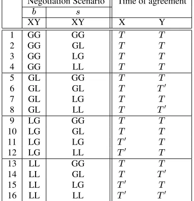
Two implementation rules are possible for this protocol [4]. One issequential implementationin which agreement on an issue is im-plemented as soon as it is settled; and the other issimultaneous implementationin which agreement is implemented only after all the issues are settled. Wefirst list the equilibrium agreements in different negotiation scenarios and then compare the outcome that results from the sequential implementation with that of the simul-taneous implementation.

Negotiation Scenario Time of agreement

XY XY X Y

1 GG GG

2 GG GL

3 GG LG

4 GG LL

5 GL GG

6 GL GL

7 GL LG

8 GL LL

9 LG GG

10 LG GL

11 LG LG

12 LG LL

13 LL GG

14 LL GL

15 LL LG

16 LL LL

[image:6.612.341.532.8.206.2]

Table 3: Equilibrium agreements for two issues X and Y

3.3 Equilibrium strategies

We assume that the conditions for convergence (as listed in sec-tion 2.4) are satisfied for both X and Y. As agents negotiate over the price of two distinct goods/services, the equilibrium strategies for the single issue model can be applied to X and Y independently of each other. The equilibrium agreements in different negotiation scenarios are listed in table 3. T equals

if (

) and

if (

).

denotes the beginning of negotiation. G indicates that the agent gains utility on time and L indicates that it loses on time. The price-surplus on both issues always goes to the agent with the longer deadline (see section 2.4).

Consider a situation where both andlose on time on X and

gain on time on Y (row 11 of table 3). Let

. Assuming the

conditions for convergence are satisfied, ’s equilibrium strategies for X and Y are

and

and those forare

and

(see table 1). During the process of negotiation, agents generate offers using these strategies. This results in an agreement on X towards the beginning of negotiation, and on Y at time

(which is the earlier deadline). The price-surplus for X and Y goes to the agent with the longer deadline, i.e., .

3.4 Implementation schemes

Any two strategies

lead to an outcome of the game. If

and

are the equilibrium strategies, then the outcome is an

agreement on X at timeand price and an agreement on Y at

time,and price. Payoffs for this outcome depend on the rules

by which agreements are implemented.

Sequential implementation. Exchange of a given good/service takes place at the time of agreement on a price for that good/service. The agents’ utilities from the strategy pair

leading

to agreements

and

,are:

,

Æ

,

Æ

(7)

the goods. The agents’utilities for this rule are:

,

Æ

,

Æ

Since the equilibrium strategies optimize the time (and price) of agreement on an issue, it seems obvious that the agents will be bet-ter off if exchange takes place sequentially rather than simultane-ously. However, since agents can have like, as well as, conflicting time preferences, it is important to determine if sequential imple-mentation proves better than simultaneous impleimple-mentation for both agents under all negotiation scenarios. We show below that sequen-tial implementation of the equilibrium agreement always gives a better outcome than simultaneous implementation.

THEOREM 2. The outcome generated by sequential implemen-tation is no worse than the outcome for simultaneous implementa-tion for both agents.

PROOF. When at least one of the agents gains on time on an issue, say X, then the equilibrium strategies result in an agreement at the earlier of the two deadlines. If

, then

and

and if

then

and

. When both

agents lose on time on X, then agreement is reached towards the beginning of negotiation. Thus

and

if

and

if

. As shown in table 3, the agents have like

time preferences in thefirst and last rows. In all other cases they have conflicting preferences on at least one issue. There are three possible ways in which agreement can be reached between agents. We analyze each of these cases below.

1. Both issues are agreed upon near the earlier deadline. Here

,. Such an agreement is possible only if, for every issue,

at least one agent gains on time. Ifandare the prices

that are agreed for X and Y, the expressions below yield equal utility from both implementation schemes to both and.

Æ

2. Both issues are agreed upon towards the beginning of ne-gotiation. This happens when both agents lose on time on both the issues. As in case 1, the expressions for utility from sequential and simultaneous schemes yield the same values

since,

.

3. One issue is agreed towards the beginning of negotiation and the other near the earlier deadline. This occurs when both agents lose on time on one of the issues, say X, and at least one agent gains on time on the other issue, say Y. Here

and the buyer’s utilities from sequential and simultaneous

implementations are:

Æ

¼

Æ

and

Æ

"

The utility from X is greater for sequential implementation since

,and both agents lose on time. The utility from Y

is equal for both schemes. As a result, sequential implemen-tation gives a total utility that is higher than simultaneous implementation. The utility that the seller gets is:

Æ

¼

Æ

and

Æ

"

Asalso loses on time on X, its utility from X is higher for

sequential implementation giving a higher cumulative utility than simultaneous implementation. Thus sequential imple-mentation always gives a better outcome than simultaneous implementation.

The same argument holds good when andnegotiate over more

than two issues. Thus from the perspective of both agents, sequen-tial implementation proves to be a better implementation scheme than simultaneous implementation.

3.5 Properties of equilibrium solution

The main focus in the design of a negotiation model is on the prop-erties of the outcome, since the choice of a model depends on the attributes of the solution it generates. We therefore study some im-portant properties [8] of the equilibrium agreement.

1. Uniqueness. If the solution of the negotiation game is unique, then it can be identified unequivocally.

THEOREM 3. For each negotiation scenario, the proposed negotiation model has a unique equilibrium agreement.

PROOF. There areindependent negotiation issues each

of which has a single equilibrium agreement (see section 2.5 for proof). This gives a unique equilibrium agreement for all

issues.

2. Symmetry. A bargaining mechanism is said to be symmet-ric if it does not treat the players differently on the basis of inappropriate criteria. Exactly what constitutes inappropri-ate criteria depends on the specific domain. The proposed negotiation mechanism possesses the property of symmetry since the outcome does not depend on which player starts the process of negotiation.

THEOREM 4. In all negotiation scenarios, the bargain-ing outcome is independent of the identity of thefirst player.

PROOF. As shown in table 3, there are two time points at which agreements can be reached;

which denotes the beginning of negotiation or T which is the earlier deadline. At these time points one of the agents (either ordepending

on whose turn it is) offers the equilibrium solution which the other agent accepts.

3. Efficiency. An agreement is efficient if there is no wasted utility, i.e, the agreement satisfies Pareto-optimality. The equilibrium solution in the proposed model is Pareto-optimal in some, but not all, negotiation scenarios.

THEOREM 5. When players have opposite time prefer-ences on an issue and the agent with the longer deadline loses on time on that issue, the equilibrium solution is not necessarily Pareto-optimal.

PROOF. Consider row 5 of table 3. Assume that

. On issue Y, the agents have conflicting time preferences. As

,

and the price-surplus in the equilibrium

solution goes to (

(8)

be increased by changing price or time or both. Price

can only be increased and, can only be decreased, since a

decrease in price or an increase in, will be unacceptable

to. An increase indecreases

and increases

. A decrease in, increases

and decreases

. But a change

in both and

, can improve both

and

. The same argument holds for the other cases.

In all the remanining scenarios it can be seen that the solution is Pareto-efficient; an increase in one agent’s uitlity lowers its opponent’s utility.

4. RELATED WORK

Fershtman [4] extends Rubinstein’s complete information model [12] for splitting a single pie to multiple pies. This model imposes an agenda exogenously, and studies the relation between the agenda and the outcome of the bargaining game. It is based on the assump-tion that both players have identical discounting factors and does not consider agent deadlines. Similar work in a complete informa-tion setting includes [5] but it endogenizes the agenda.

Bac and Raff [1] developed a model that has an endogenous agenda. They extend Rubinstein’s model [13] for single pie bar-gaining with incomplete information by adding a second pie. In this model the price-surplus is known to both agents. For both agents, the discounting factor is assumed to be equal over all the issues. One of the players knows its own discounting factor and that of its opponent. The other player knows its own discounting factor but is uncertain of the opponent’s discounting factor. This can take one of two values,Æ

with probability andÆ

with probability . These probabilities arecommon knowledge. Thus agents

have asymmetric information about discounting factors. They how-ever do not associate deadlines with players.

The difference between these models and ours is thatfirstly, our model considers both agent deadlines and discounting factors. Sec-ondly, in our case the players are uncertain about the opponent’s reservation price and deadline. Each agent knows its own reserva-tion price and deadline but has a binary probability distribureserva-tion over its opponent’s reservation price and deadline. Moreover, the dis-counting factor is different for different issues and the players have no information about the opponent’s discounting factors. Thirdly, each agent’s information state is itsprivate knowledgewhich is not known to its opponent. Our model is therefore closer to most real life bargaining situations than the other models. The fourth point of difference lies in the attributes of the solution. Comparing the solu-tion properties of these models, we see that the existing models do not have a unique equilibrium solution. The equilibrium solution depends on the identity of thefirst player. In our model, the equi-librium solution is unique and is independent of the identity of the

first player. However, as is the case with our model, the equilibrium solution is not always Pareto-optimal in the other models.

5. CONCLUSIONS

This paper presented a model for multi-issue negotiation under time constraints in an incomplete information setting. The order in which issues are bargained over and agreements are reached is determined endogenously as part of the bargaining equilibrium rather than im-posed exogenously as part of the game tree. An important property of this model is the existence of a unique equilibrium. For any is-sue, this equilibrium results in agreement at the earlier deadline if at least one agent has the incentive to reach a late agreement and at the beginning of negotiation if both agents have the incentive to reach an early agreement. The price-surplus on all issues goes to the agent with the longer deadline.

The sequential implementation of the equilibrium agreement was shown to result in an outcome that is no worse than the outcome for simultaneous implementation when agents have similar, as well as conflicting, time preferences. The equilibrium agreement possesses the properties of being unique and symmetric, although it is not always Pareto-optimal.

As it currently stands, our model considered the negotiation is-sues to be independent of each other. In future we intend to study bargaining over interdependent issues. Apart from this, our model considered the case where agents had uncertain information about each other’s deadline and reservation price. In future we will in-troduce learning into the model that will allow the agents to learn these parameters during negotiation. These extensions will take the model further towards real life bargaining situations.

6. REFERENCES

[1] M. Bac and H. Raff. Issue-by-issue negotiations: the role of information and time preference.Games and Economic Behavior, 13:125–134, 1996.

[2] P. Faratin, C. Sierra, and N. R. Jennings. Negotiation decision functions for autonomous agents.International Journal of Robotics and Autonomous Systems,

24(3-4):159–182, 1998.

[3] S. S. Fatima, M. J. Wooldridge, and N. R. Jennings. Optimal negotiation strategies for agents with incomplete

information. InATAL-2001, pages 53–68, Seattle, USA, 2001.

[4] C. Fershtman. The importance of the agenda in bargaining.

Games and Economic Behavior, 2:224–238, 1990. [5] R. Inderst. Multi-issue bargaining with endogenous agenda.

Games and Economic Behavior, 30:64–82, 2000. [6] R. Keeney and H. Raiffa.Decisions with Multiple

Objectives: Preferences and Value Tradeoffs. New York: John Wiley, 1976.

[7] A. Lomuscio, M. Wooldridge, and N. R. Jennings. A classification scheme for negotiation in electronic commerce. In F. Dignum and C. Sierra, editors,Agent-Mediated Electronic Commerce: A European Agentlink Perspective., pages 19–33. Springer Verlag, 2001.

[8] M.J.Osborne and A. Rubinstein.A Course in Game Theory. The MIT Press, Cambridge, England, 1998.

[9] R. P. Maes and A.G.Moukas. Agents that buy and sell.

Communications of the ACM, 42(3):81–91, 1999. [10] D. G. Pruitt.Negotiation Behavior. Academic Press, 1981. [11] H. Raiffa.The Art and Science of Negotiation. Harvard

University Press, Cambridge, USA, 1982.

[12] A. Rubinstein. Perfect equilibrium in a bargaining model.

Econometrica, 50(1):97–109, January 1982. [13] A. Rubinstein. A bargaining model with incomplete

information about time preferences.Econometrica, 53:1151–1172, January 1985.

[14] T. Sandholm. Agents in electronic commerce: component technologies for automated negotiation and coalition formation.Autonomous Agents and Multi-Agent Systems, 3(1):73–96, 2000.

[15] T. Sandholm and N. Vulkan. Bargianing with deadlines. In

Multi issue negotiation under time constraints