B. Image acquisition



Abstract—This paper reports on observations of the distribution of micro-structural features in a sample of cortical bone (mid-diaphysis femur from bovine). Such features include lacunae, Haversian canals, and canaliculi clusters and are considered, upon bone treatment, to be porosities. Initially, image segmentation was utilized to quantify feature geometric attributes such as area A (µm2), perimeter P(µm), elliptical ratio min/maj axis length, and compactness. A center point of the bone cross section was determined from which a polar coordinate system was constructed related to which was a grid containing 25 regions of roughly 500x500 µm in size. Distributions of these features were plotted vs. distal radius and vs. angular positions as measured from the center of the bone. Analyses of the linear trends reveals that all porosity attributes and for all feature types (Haversian canals, and canaliculi clusters) appear to decrease fairly linearly with increasing radius from bone center (p< 0.05%) as the outer perimeter is reached. Also, these features tend to become more round (p< 0.05%) as they get closer to the outer shell. In contrast, the geometric attributes appear to be indifferent vs. the angle.

Index Terms— Image segmentation, cortical bone microstructure, size, shape, radius, angle.

I. INTRODUCTION

aversian canals, lacunae and canaliculi represent the major constituents of the total porosity in cortical bone [1]. These porous micro-features are characterized by non-uniform distribution through the cortical width [2, 3]. Distribution of such features has been reported to contribute toward bone mechanical integrity, the higher the density of those cavities the weaker is the bone [4, 5].

Since the alteration of the micro-structural geometric distribution in the cortical bone affects its mechanical integrity [6], the aim of this paper is to investigate the geometrical distribution of such porous micro-structures in the cortical bone and to develop a relationship that links the geometrical properties size and shape (e.g.: area, compactness, perimeter, and ratio) of the porosities (lacunae, Haversian canals, and canaliculi clusters) to the radial distance from the bone center using imagery.

Manuscript received March 06, 2014; revised March 29, 2014. I. S. Hage is a PhD student in the Mechanical Engineering Department at the American University of Beirut, Riad-El Solh, Beirut 1107 2020 Lebanon (e-mail: [email protected])

R. F. Hamade is a Professor of Mechanical Engineering at the American University of Beirut, Riad-El Solh, Beirut 1107 2020 Lebanon (corresponding author to provide phone: 961-1-374 374 ext. 3481; e-mail: [email protected]).

An image segmentation methodology developed by the authors [7, 8, 9] is utilized here to automatically segment cortical bone images captured at different polar and linear positions from center of the bone. Each micro-constituent of the bone was separated in 25 adjacent images of roughly 500x500 m in size. The geometrical properties in each image were extracted and related to the polar coordinate where the image was captured.

II. MATERIALS

A. Sample preparation

Bones were extracted from bovine animal femur (2-year-old cow collected fresh from a butcher). The bone samples were pathologically prepared where for better visualization; slices were exposed to Hematoxylin and Eosin (H&E) staining solution. Fig. 1 illustrates the preparation steps of the bone sample, where shown in figure 1 a) is the position where the slice was cut with a polar coordinate system is assigned with marked origin and the angular/radial directions. Fig. 1 b) represents the bone after staining. Fig. 1 c) and d) show the images captured with an Olympus optical microscope at 5X and 20X magnifications respectively. B. Image acquisition

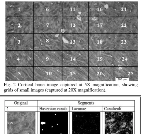
BX-41 M LED optical microscope, equipped with an SC-30 digital camera was used to capture images. Fig. 2 shows an image at 5X magnification, this image was gridded into 25 images where each one of the 25 images is captured at 20X for the purpose of better detection of the micro-constituents of the bone.

III. IMAGE SEGMENTATION

An image segmentation technique based on pulse coupled neural networks (PCNN) combined with adaptive threshold (AT) and PSO optimization is used to automatically discern the micro-features of cortical bone histology [9,10]. The fitness function for the PSO optimization algorithm was based on geometric attributes [9, 10]. Each of the 25 images was segmented based on the methodology advanced in [7]. Fig. 3 shows samples of the images considered for segmentation as they are prepared as 25 adjacent blocks.

Observations on the Geometric Distribution of

Micro-structural Features in Cortical Bone

I. S. Hage, R. F. Hamade

IV. METHODOLOGY

Based on Fig. 1 a) a polar coordinate system was adopted to identify the location of the bone micro constituents. The distance between the origin and the inner diameter of the bone (image b) in Fig. 1) was measured using a digital caliper to be 1.2 cm or (12000µm). The 20x images where localized in the coordinate system by using the calibrated scale bar of the microscope (the dimensions of the images in pixels (2048*1532 pixels2) were converted to µm2 (575*430 µm)) thus the radius and angle for the center of each image was calculated and each image was assigned radial coordinates.

Following geometrical attribute identification procedure described in [9], values of the area, perimeter, compactness, and ratio (of elliptical major/minor axis length) were calculated for each of the three bone micro-constituents at different R/Θ locations.

V. RESULTS

Based on Fig. 4, images that share the same angle are the following images:

 Images 15,20,24 at the same angle θ1: 104.4817

 Images 14,19,23 at the same angle θ2: 105.9967

 Images 9,13,18 at the same angle θ3: 107.27

 Images 8,17 at the same angle θ4: 108.5867

 Images 3,12 at the same angle θ5: 109.3032

 Images 2,7 at the same angle θ6: 110.4283

 Images 6,11 at the same angle θ7: 111.3775 Based on Fig. 4 images that are at the same distal radius are the following imgaes:

 Images 11, 17, 23 at the same radius R1: 1.60860

 Images 6, 12, 18, 24 at the same radius R2:1.64075

 Images 7, 13, 19 at the same radius R3: 1.671513

 Images 2, 8, 14, 20 at the same radius R4: 1.70378

 Images 3, 9, 15 at the same radius R5: 1.733987 The values of total area, total perimeter, average ratio, and average compactness of the three porosities in each image were calculated and were plotted versus the angle Θ and the radius R.

A. Area

Areas of the Haversian canals, lacunae and canaliculi versus Θ at different radius

The areas of the individual micro porosities (Haversian canals, lacunae and canaliculi) in each image were calculated then their sum was plotted versus the angle Θ at all the radii. Fig.5 shows the results.

Fig. 1. Bone sample preparation and imaging a) the section cut showing the polar coordinate system and the position where the slice was cut, b) the slice after pathological processing, c) the image captured at 5x magnification, d) one of the images captures at 20x magnification

Fig. 2 Cortical bone image captured at 5X magnification, showing grids of small images (captured at 20X magnification).

Fig. 3 Resultant segments of some of the images shown in Fig. 2

Fig. 4 Bone images of the grids shown in Fig. 2 captured at 20X magnification

Total Area Haversian canals

Total Area Lacunae

Total Area Canaliculi

Fig. 5 The area of the Haversian canals, lacunae and canaliculi vs. θ for all distal values (cm): R1=1.608603, R2= 1.640754, R3= 1.671513, R4= 1.70378, R5= 1.733987

Areas of the Haversian canals, lacunae and canaliculi versus R at different angles

The areas of the Haversian canals, lacunae and canaliculi were plotted versus the radius Rat all the angles, Fig.6 show the results.

Total Area Haversian canals

Total Area Lacunae

Total Area Canaliculi

Fig. 6 The area of the Haversian canals, lacunae and canaliculi vs. R(cm) for all angles: ϴ1=104.4817, ϴ2=105.9967, ϴ3= 107.27, ϴ4= 108.5867, ϴ5= 109.3032, ϴ6=110.4283, ϴ7=111.3775

The area vs. R were fitted using linear trend. Table 1 shows the results of the trends obtained as well as the corresponding statistical analysis for each linear regression where R is the radius in cm, A is the area in µm2. The area vs. angle were fitted using constant linear trends.

B. Perimeter

Perimeter of the Haversian canals, lacunae and canaliculi versus Θ at different radius

The perimeters of the individual micro porosities (Haversian canals, lacunae and canaliculi) in each image were calculated then their sum was plotted versus the angle Θ at all the radii. Fig.7 shows the results.

Total Perimeter Haversian canals

Total Perimeter Lacunae TABLEI

STATISTICAL ANALYSIS OF THE TOTAL AREA LINEAR REGRESSIONS

Linear fit Coefficients R2 _p-value

Total Perimeter Canaliculi

Fig. 7 The perimeter of the Haversian canals, lacunae and canaliculi vs. θ for all distal values (cm): R1=1.608603, R2= 1.640754, R3= 1.671513, R4= 1.70378, R5= 1.733987

Perimeter of the Haversian canals, lacunae and canaliculi versus R at different angles

The perimeter of the Haversian canals, lacunae and canaliculi were plotted versus the radius Rat all the angles. Fig.8 shows the results.

Total Perimeter Haversian canals

Total Perimeter Lacunae

Total Perimeter Canaliculi

Fig. 8 The perimeter of the Haversian canals, lacunae and canaliculi vs. R(cm) for all angles: ϴ1=104.4817, ϴ2=105.9967, ϴ3= 107.27, ϴ4= 108.5867, ϴ5= 109.3032, ϴ6=110.4283, ϴ7=111.3775

The perimeter vs. R were fitted using linear trend. Table 2 shows the results of the trends obtained as well as the corresponding statistical analysis for each linear regression where R is the radius in cm, P is the perimeter in µm. The area vs. angle were fitted using constant linear trends.

C. Ratio

Ratio of the Haversian canals, lacunae and canaliculi versus Θ at different radius

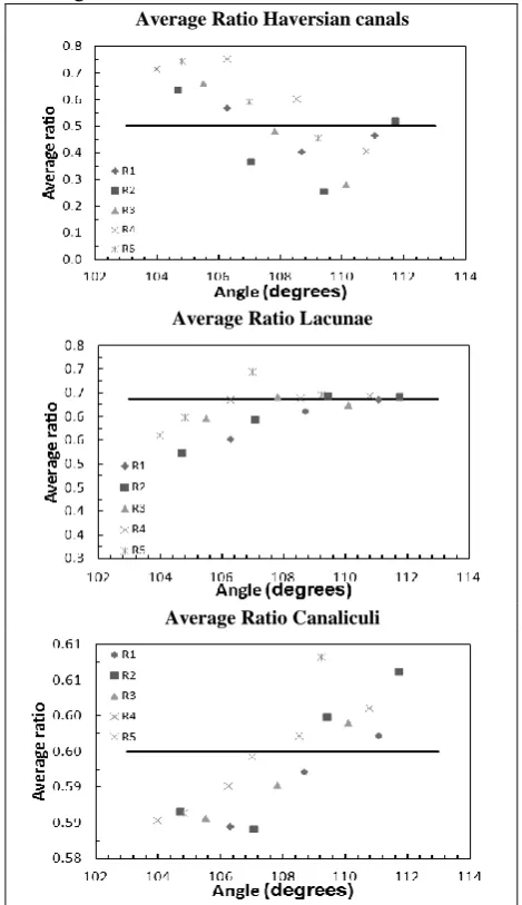
The ratios of the individual micro porosities (Haversian canals, lacunae, and canaliculi) in each image were calculated. The values were averaged and plotted in Fig. 9 versus angle Θ at all the radii.

Average Ratio Haversian canals

Average Ratio Lacunae

Average Ratio Canaliculi

Fig. 9 The ratio of the Haversian canals, lacunae and canaliculi vs. θ for all distal values (cm): R1=1.608603, R2= 1.640754, R3= 1.671513, R4= 1.70378, R5= 1.733987

TABLEII

STATISTICAL ANALYSIS OF THE TOTAL PERIMETER LINEAR REGRESSIONS

Linear fit Coefficients R2 _p-value

Ratio of the Haversian canals, lacunae and canaliculi versus R at different angles

The ratio of the Haversian canals, lacunae and canaliculi were plotted versus the radius Rat all the angles. Fig.10 shows the results.

Average Ratio Haversian canals

Average Ratio Lacunae

Average Ratio Canaliculi

Fig. 10 The ratio of the Haversian canals, lacunae and canaliculi vs. R(cm) for all angles: ϴ1=104.4817, ϴ2=105.9967, ϴ3= 107.27, ϴ4= 108.5867, ϴ5= 109.3032, ϴ6=110.4283, ϴ7=111.3775

The ratio vs. R were fitted using linear trend. Table 3 shows the results of the trends obtained as well as the corresponding statistical analysis for each linear regression where R is the radius in cm, r is the ratio. The area vs. angle plots were fitted using constant linear trends.

D. Compactness

Compactness of the Haversian canals, lacunae and canaliculi versus Θ at different radius

The compactness of the individual micro porosities (Haversian canals, lacunae and canaliculi) in each image were calculated then the average was plotted versus the angle Θ at all the radii. Fig.11 shows the results.

Average Compactness Haversian canals

Average Compactness Lacunae

Average Compactness Canaliculi

Fig. 11 The compactness of the Haversian canals, lacunae and canaliculi vs. θ for all distal values (cm): R1=1.608603, R2= 1.640754, R3= 1.671513, R4= 1.70378, R5= 1.733987

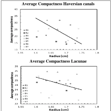
Compactness of the Haversian canals, lacunae and canaliculi versus R at different angles

The compactness of the Haversian canals, lacunae and canaliculi were plotted versus the radius Rat all the angles. Fig.12 shows the results.

Average Compactness Haversian canals

Average Compactness Lacunae TABLEIII

STATISTICAL ANALYSIS OF THE AVERAGE RATIO LINEAR REGRESSIONS

Linear fit Coefficients R2 p-value

Haversian r=2.2372*R-3.2766 R^2=0.9673 0.00127

Average Compactness Canaliculi

Fig. 12 The compactness of the Haversian canals, lacunae and canaliculi vs. R(cm) for all angles: ϴ1=104.4817, ϴ2=105.9967, ϴ3= 107.27, ϴ4= 108.5867, ϴ5= 109.3032, ϴ6=110.4283, ϴ7=111.3775

Compactness vs. R plots were fitted using linear trend lines. Table 4 shows the results of the trends obtained as well as the corresponding statistical analysis for each linear regression where R is radius in cm, C is compactness. Plots of area vs. angle were fitted using linear trends.

VI. INTERPRETATION OF RESULTS

Examining figures 5, 7, 9 and 11 which represent the area, perimeter, ratio, and compactness, respectively, for the Haversian canals, lacunae and canaliculi clusters vs. θ at different radii, the geometric characteristics were practically horizontal vs. angle. One may conclude that no effect exits of θ on the porosities geometric attributes. This is logical since bone growth in thickness occurs by building radial cortical shells, thus by varying θ (circularly) the composition of the bone would be the same, and within the same radius by varying the angle θ from 0º to 360º the bone microstructure would not change.

On the contrary, figures 6, 8, 10 and 12 which represent the porosities’ geometric characteristics vs. R at different angles θ, show definite trends where:

1- For the shape properties, compactness values appear to decrease and the ratio increase with R (from the inner to the outer radius). As compactness values approach 12.5 (or ratio approaches unity) [9], features tend to be circular. this finding suggests that the outer shell of the cortical bone contains porosities that are more round than those present in the inner cortical regions.

2- For the size properties, the total area and perimeter decreased with R almost linearly which appears to give the cortical bone its toughness. This decrease in porosity is in line with those reported by other authors in [11, 12]. The trend of the geometric properties is approximated using linear trends with calculated p< 0.05 values illustrating a statistical significance of such decreasing trends.

VII. CONCLUSIONS

For cortical bone, reported in this paper are preliminary observations on the geometric characteristics (area, perimeter, ratio, and compactness) of the micro-features

(Haversian canals, lacunae, and canaliculi) present in relation to position within the cortical bone. This position is determined with respect to a polar system centered on the geometric center of the bone cross section. Geometric characteristics of micro features were extracted from optical images at 20X magnification using an image segmentation methodology proposed previously by the authors. The geometric characteristics are plotted as function of the distal radius and polar angle.

While values of geometric characteristics are found to be independent with respect to angle θ, they appear to vary greatly when plotted against bone radius, R. For example, porosity decreases greatly with increasing radius. Area A (µm2) and perimeter P(µm) of the porosities was found to decrease linearly for the lacunae A=-1050.1*R+2061.3/ P=-3796.8*R+7388.5, for the Haversian canals A=-11547*R+21118/ P=-369.35*R+750, and for the canaliculi A=-71713*R+137667/ P=-82454*R+164028R where R is the radius from bone center (in cm)).

Compactness values were found to decrease and the values of the ratio measure to increase as function of radius suggesting that porosities tend to become more circular as they near the outer shell of the cortical bone. The compactness, C, and the ratio, r, of the porosities were found to decrease almost linearly for the lacunae C=-9.005*R+39.258 /r=0.828*R-0.7759, for the Haversian canals C=-129.021*R+240 / r=2.2372*R-3.2766, and for the canaliculi C=-2.6089*R+31.8/ r=0.0521*R+0.5085. The outer shell of the cortical bone appears to contain more circular-shaped porosities than the inner regions.

REFERENCES

[1] P. Atkinson, "Changes in resorption spaces in femoral cortical bone with age," J. Pathol. Bacteriol., vol. 89, pp. 173-178, 1965. [2] V. Bousson, A. Meunier, C. Bergot, É. Vicaut, M. A. Rocha, M. H.

Morais, A. Laval‐Jeantet and J. Laredo, "Distribution of intracortical porosity in human midfemoral cortex by age and gender," Journal of

Bone and Mineral Research, vol. 16, pp. 1308-1317, 2001.

[3] M. L. Bouxsein and D. Karasik, "Bone geometry and skeletal fragility," Current Osteoporosis Reports, vol. 4, pp. 49-56, 2006. [4] I. S. Hage and R. F. Hamade, "Micro-FEM orthogonal cutting model

for bone using microscope images enhanced via artificial intelligence," Procedia CIRP, vol. 8, pp. 384-389, 2013.

[5] I. S. Hage and R. F. Hamade, "Segmentation of histology slides of cortical bone using pulse coupled neural networks optimized by particle-swarm optimization," Comput. Med. Imaging Graphics, vol. 37, pp. 466-474, 2013.

[6] R. B. Martin, "Porosity and specific surface of bone," Crit. Rev.

Biomed. Eng., vol. 10, pp. 179-222, 1984.

[7] R. McCalden, J. McGeough and M. Barker, "Age-related changes in the tensile properties of cortical bone. The relative importance of changes in porosity, mineralization, and microstructure," The Journal of Bone & Joint Surgery, vol. 75, pp. 1193-1205, 1993.

[8] W. Sietsema, "Animal models of cortical porosity," Bone, vol. 17, pp. S297-S305, 1995.

[9] I. S. Hage and R. F. Hamade, "Geometric-attributes-based segmentation of cortical bone slides using optimized neural networks," submitted.

[10] I. S. Hage and R. F. Hamade, "Detecting Individual Osteons in histology cortical bone slides using PSO-optimized PCNN," submitted.

[11] D. Thompson, "Age changes in bone mineralization, cortical thickness, and haversian canal area," Calcif. Tissue Int., vol. 31, pp. 5-11, 1980.

[12] R. Zebaze, A. Ghasem-Zadeh, A. Bohte, S. Iuliano-Burns, M. Mirams, R. I. Price, E. J. Mackie and E. Seeman, "Intracortical remodelling and porosity in the distal radius and post-mortem femurs of women: a cross-sectional study," The Lancet, vol. 375, pp. 1729-1736, 2010.

TABLEIV

STATISTICAL ANALYSIS OF THE AVERAGE COMPACTNESS LINEAR REGRESSIONS

Linear fit Coefficients R2 _p-value