Nonlinear adaptive filter performance in typical applications

Pergamon

A. Rev. Control, Vol. 20, pp. 107-118, 1996 ©International Federation of Automatic Control 1997 S0066-4138-97-000 ~ - ~ = ( ) 09-8 Printed in Great Britain. All rights reserved 1367-5788/97 $32.00 + 0.00

NONLINEAR ADAPTIVE FILTER PERFORMANCE IN TYPICAL APPLICATIONS

Peter M. Grant, S. Chen I and B. Muigrew

Electrical Engineering, University of Edinburgh, Edinburgh, Scotland now at Electrical Engineering, University of Portsmouth, Portsmouth, UK

Abstract: This paper examines approaches to the realisation of nonlinear filters as used in signal and image processing. The design of adaptive nonlinear processors is examined and their application as adaptive equalisers to alleviate bandlimiting, distortion and interference in a typical communications channel is investigated. This paper re-examines the equalisation process as one which seeks to correctly classify the channel output into one of a finite and known alphabet of symbols encompassing the data at the channel input. The optimal solution for this classification problem is shown to be inherently nonlinear. Several nonlinear structures are examined, which allow much more complex classification boundaries, and provide greatly enhanced performance for the nonlinear filter over the more conventional linear filter. Finally the use of a nonlinear predictor is investigated for time series analysis.

Keywords: adaptive filter, adaptive equaliser, neural network, nonlinear filter, prediction methods

1. INTRODUCTION

Linear processors are bounded by the fact that the output is formed by a weighted sum of the input sig- nal values or samples. They are a restricted class of systems but they do predominate in most electronic communication systems, The linear property means that the response to a sum of two or more inputs is equal to the sum of the responses to the individual inputs, as is implied in the principle of superposition. Systems are often not only linear but also time invari- ant, in that their properties such as gain etc, hopefully do not alter with time.

Many electronic components, however, only provide linear operation over a restricted range of (small) sig- nals and when the signal amplitude increases then the system becomes nonlinear. This is clearly true in an amplifier as the signal magnitude approaches the power supply voltages then saturation in the gain stages introduces limiting or clipping and the output signal is no longer related, in a linear manner, to the input signal, Figure 1.

In electronics there are many phenomena which cause the system output to be nonlinearly related to the input. The diode detector and rectifier both have a nonlinear characteristic. Other significant nonlinear

effects arise from non-Gaussian or impulsive noise. Film for recording images as well as photodetectors are nonlinear, as is the human perception system. In this latter case the logrithmic nonlinearities in human vision system are vital to achieve the large dynamic range and permit it to handle the wide range of input signals. Many other image processing operations, such as maximum entropy restoration, are nonlinear, as is the corresponding speech system which is used to represent efficiently the PCM encoded signals.

0"%

INPUT

OUTPUT

(i) ~

(c)

H k

o

(b) ~

" ~

Ill

"~)""

+

Vt~

.~..V...~...V... o v

OV

Fig. 1 Nonlinear distortion in an amplifier.

107

108 Adaptive Systems

signal types.

2. FILTERS FOR NOISE REDUCTION

It is widely realised that if a signal is corrupted by wideband noise then the noise can he reduced by lowpass filtering. Lowpass filters can he designed into finite impulse response (FIR) filters by appropri- ate design and selection of the weight coefficient val- ues, h,, Figure 2. The relationship between the filter input,

x(k),

N-I

y(k) = ~

hix(k-i)

where N is the number of weights in the filter.

Unfortunately to he effective the passband width must he narrow and this often distorts the signal. In image processing, where a 2-dimeusional filter i s used, the effect of the iowpass operation removes all the high frequency components which are associated with edge features. Thus the filtered image will have blurred edges. The image processing

community

hN~

Fig. 2 Finite impulse filter.

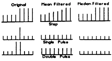
The 1-D median FIR filter processes an odd number of pixels or samples and it rank orders the magni- tudes of the samples from the largest to the smallest and outputs the middle or median value. This is clearly a nonlinear filter as the output is based on the statistics of the input data. This median filter is espe- cially useful in impulsive noise provided that the number of noise samples encountered is less than half the number of samples or pixels being processed in the filter. Features such as edges are largely unaf- fected by the processing. Figure 3 shows a schematic example of a 1-D input signal as filtered in a lowpass (mean) and median filter.

More recently interest has focussed on weighted median filters (Gabbonj) and stack filters (Coyle). In the weighted median filter a non-negative integer weight is assigned to each position in the filter win- dow, as in the FIR filter, prior to the rank order opera- tion. These structures are particularly important when the filter is to be adaptive and the weights have

to be

shown in the processed speech waveform of Tabus, Figure 4. Other work on 2-D images (Yin) compares the mean square and mean absolute errors in lowpass, median and weighted median filters, where consider- able performance improvements are obtained over the simple median filters.

O r i j ~ r m l M e a n F i l l e r e d I ' l e d ~ . F t l l e r e d

,,,,IILI ,,111111 ,,,,llil

S t e p

I I I I [ I I I

l l l l l l l l

l l I I s l l l

, , l , , , I I I I I I I I , , , , , , , ,

De4~bb PtAse

Fig. 3 Linear mean and nonlinear median filtering.

(b)

~ j ~ 'lm~ ~ ~

7 ~ 7000 7960 8000

?mOO 7ISO ?llO0 7HO iO00

Fig. 4 Noise reduction in speech, courtesy Tabus. (a) I0 s of speech signal with added (dotted) burst errors, (b) error after 3-point median filtering as in Fig. 3, (c) reduced error after using the filter of Tabus.

Adaptive Systems 109

Stack filters with boolean operations are particularly important for efficient VLSI implementation of high

speed

3. ADAPTIVE EQUALISATION

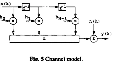
input, x ( k ) , and the channel output, y(k), can be sum- m a r i ~ in the following extended equation:

N-!

y(k) = ~, hix(k - i) + n(k) (2)

b,O

Adaptive channel equalisation is an old problem for which a variety of solutions have been proposed and attempted (Qureshi). There is always a commercial demand to increase the capacity of existing commw nications channels and to operate in more difficult environments with more severe levels of intersymbol interference (ISI), co-channel interference, additive noise and Doppler spread.

This paper re-examines the equalisation process as one which seeks to correctly classify an observed sequence (the channel output) into one of a finite and known alphabet of symbols (the data at the channel input). It demonstrates that by adopting a Bayesian approach an optimum decision boundary can be defined by certain probability density functions - effectively defining an optimal nonlinear equaiiser as a mapping from observations to decisions. A geomet- ric visualisation of classification highlights the short- comings of the linear equaliser.

Now explore techniques for constructing the nonlin- ear equaliser starting with the multilayer percepu'on (MLP) or neural network. Greatly enhanced perfor- mance can be achieved using this highly nonlinear structure. We demonstrate how the polynomial-based Volterra.filter can also be configured as an equaliser and how its performance compares with that of the MLP. Finally, a radial basis function (RBF) structure is examined and it is show to be a more natural solu- tion.

z

~

n(k)

Fig. $ Channel model.

Many digital communications channels are subject to intersymbol interference (ISI), due to restricted band- width and/or the presense of muitipath distortion in the transmission medium. Many such channels can be characterised by a FIR digital channel filter and an additive noise source, Figure 5. The observed sequence, {y(k)}, is formed by adding Ganssian ran- dora noise to the output of the FIR channel filter, of equation (I). The relationship between the channel

Essentially, the equalisation problem is that of using the information present in the observed channel out- put vector

y(k) = [y(k) y ( k - 1 ) . - . y ( k - M + 1)] r (3)

to produce an estimate, :t(k - d), of the channel input

x ( k - d), as illuslrated in Figure 6. The device or algorithm which performs this function is the equaliser which has order M and operates with lag (delay) d, Figure 6.

n(k)

(k-d)

Fig. 6 Generic equaliser structure.

4. A CLASSIFICATION PROBLEM

In order to exploit the characteristics of the transmit- ted sequence more fully it is appropriate to highlight the finite state nature of the channel itself. To sim- plify the development we will assume that the trans- mitted sequence is binary with equal probability. For the simple case where the channel has 2 coefficients and the equaliser vector y(k) has 2 elements, we can summarise all possible channel output vectors by the following equation:

r

,(k)

]_[ho h,

+

ho

j

which can be written more compactly as

y(k) = H x(k) + n(k) = 9(k) + n(k) (5)

110 Adaptive S y s t e m s

X(k) x(k- I) x ( k - 2 ) ,, ,,,,

-1 - ! - I

-1 -1 +1

- I +1 - I

- I +1 +1

+1 -1 - ! + i - i +! +1 +1 - i

+1 +1 +1

9(*)

-1.5 - ! . 5 -0.5 .0.5

~(A-l)

-1,5 -0.5 -~0,5 +1.5

40.5 -1.5 +0.5 .0.5 +!.5 ~1.5 +1.5 +1.5

Table I Noise-free outputs for channel n(:)= I +o. s:".

A

I

-i

-2

! I

" ~ ( k ) = - I

×

X

I l

-2 -I

I / I I

2 (k) - + i

/

/ , , n 2 - O . 01

.

' n 2 - 0 . 2

t •

'~n2-O. 5

/

t

,i I I I

0 1 2

y(k)

Fig, 7 Observation space formed by two successive outputs from channel H ( z ) = l + 0 . 5 z -I. Dashed line: linear decision boundary, solid curves: optimal decision boundaries with different values of noise v a r i a n c e n 2.

Figure 7 shows each of these 8 possible points plot- ted as either a × to indicate that the output vector rep- resents an input

x(k)

x(k) = +1. When we add noise to the vector ~(k), the 8 points become 8 clusters where the displayed points are the means or centres of the clusters. Thus the equalisation problem now involves the assigning of regions within the observation space spanned by the noisy channel output vector y(k) to represent inputs of either x(k) = +1 or x(k) = -1.

The linear equaliser performs such a classification in conjunction with a decision device or slicer. The decision boundary is the locus of all values of y(k) for which the output of the linear filter is zero. The decision device in this simple case is a sign function and when y(k) has only two elements, it is a straight (dashed) line in Figure 7 which divides the space into two regions. All observation vectors to the right of line will be classified as indicating that

x(k)

all points to the left of the line as

x(k)

example the points y = [-0.5 0.5] r and

y = [1.5 0.5] r. The point associated with a -1 deci- sion is closer to the boundary than the point associ- ated with a +1 decision. Therefore, in the presence of noise, there is a higher probability of a channel out- put vector centred on [-0. 5 0. 5] r being incorrectly detected as a +I than a channel output centred on [l. 50. 5] r being incorrectly detected as a - I . This is clearly a non-optimum strategy.

This geometrical description of the shortcomings of the linear equaliser leads us directly to a Bayesian approach (Chert, 1990IEE). Having observed a vec- tor y(k), if the probability that it was caused by x ( k - d ) =+1 exceeds the probability that it was caused by x ( k - d ) - - l , then we should decide in favour of +1 and vice versa. The optimal decision boundary is the locus of all values of y(k) for which the probability that x ( k - d ) = +1 given a value for y(k) is equal to the probability that x ( k - d ) - - 1 given the same y(k). More formally, the decision boundary can be defined as the solution to a condi- tional probability equation, which leads to the follow- ing nonlinear equaliser function (Chert, 1990IEE) based on the difference of conditional density func- tions:

.e(k - d) = sgn ( py,x(y(k)lx(k - d) -- + l ) -

p~(y(k)lx(k - d) = -1) ) (6) The density functions and hence the equaliser can now be derived directly from the generation mecha- nism summarised in equation (4). The decision boundary defined by this analysis is illustrated for various levels of noise in Figure 7. For low levels of noise the boundary is piecewise linear but it becomes more smooth as the noise level increases. Clearly to equalise this channel we require to use a nonlinear filter.

The above geometric analysis can easily be applied to the general equaliser structure of Figure 6. In general, the optimal Bayesian decision boundary is a hyper- surface in the M-dimensional observation space and the realization of this nonlinear boundary requires nonlinear decision capability. The linear equaliser can however only implement a hyperplane decision boundary.

5. THE MULTILAYER PERCEPTRON

Adaptive Systems 111

The basic building block of the MLP is the single neuron or node which is shown in Figure 8. A node receives a number of inputs x l , " ", x,, say, which are then multiplied by a set of weights w l , " ", wn and

the resultant values are summed. A constant O, known as the node threshold, is added to this weighted sum of inputs, and the output of the node is obtained by evaluating a nonlinear function, f , of the total. The output mapping function is the operation which makes this processor nonlinear. We focus our attention on nodes where the node activation func- tion, f , is defined by

f(x) = (1 -e-X)l(l + • -x) (7)

the graph of which is also shown in Figure 8.

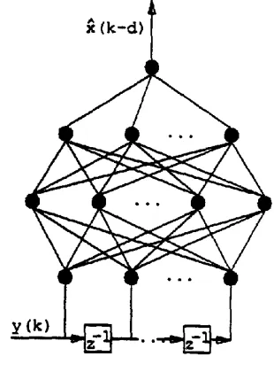
learn a task adaptively, MLPs can be trained by m e a n s of the back-propagation (BP) algorithm (Rumelhart). This is a simple stochastic gradient- descent algorithm similar to that used in linear equalisers (Qureshi).

The major difficulty with the MLP is that training is essentially a nonlinear optimisation problem. The mean squared error surface is multi-modal and hence it is exlremely difficult to design gradient type algo- rithms which are guaranteed to find the global mini- mum under all input signal conditions, hence the next algorithm development.

x±" w ±",,~

Xn:" °

f(x)

~ X

- 1

Fig. 8 Node structure and activation function.

In the MLP a number of nodes are arranged in layers, as depicted in Figure 9. A multi-dimensional input is passed to each node in the first layer. The outputs of the first layer nodes then become inputs to the nodes in the second layer, and so on. The output of the net- work is therefore the outputs of the nodes lying in the final layer. Thus, weighted connections exist from a node to every node in the succeeding layer, but no connections exist between nodes in the same layer. Since an equaliser usually has one output the network has a single node in the output layer.

MLPs which have three layers are essentially capable of forming any desired decision region (Gibson, 1990), and it is this property which makes them attractive as nonlinear equalisers. When required to

Fig. 9 Multilayer perceptron equaliser.

The slab algorithm (Hassell Sweatman et al. 1994) is a deterministic design method for constructing a 2 layer MLP from McCulloch and Pins units i.e. the node activation function of equation (7) is

f ( x ) = sgu(x) and is such that the node output is either +1 or -1. The output of the ith node in the hid- den layer is typically:

sgu(yr(k) w i - Oi )

where w i is the vector of weights on the input to the ith node and Oi is the threshold. The algorithm requires knowledge of the noise free states or equiv- alently the channel impulse response and application of linear programming techniques.

112 Adaptive Systems

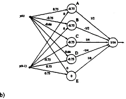
are associated with a +1. If A and B are the same hyperplane then the states are linearly seperable, as the hyperplanes are identical and the common hyper- plane defines the coefficients of a linear equaliser. If the states are not linearly seperable the space between the two lines is "slab 1". The width of the slab is chosen to minimise the number of states within it. The hyperplanes A and B define two nodes on the MLP structure illustrated on Figure 10Oa). The weights on the input to the second layer o f the network are now taken from a geomeuic series. In this case any decision made by nodes A and B will dominate the final decision and they have significant weight values (½). Thus if the input vector y(k) is to the left of hyperplane A an output decision o f + l will result. If the vector is to the right of B an output decision of -1 will result. Finally if the vector is within slab 1, nodes A and B will contribute a total of 0 to the output node and will not affect the final deci- sion.

~t.I)

0.75

(b)

Fig. 10 MLP constructed by the Slab algorithm for channel H ( z ) = O . 3 3 3 + O . 6 6 7 z - I + z - 2 : (a) state structure and resultant hyperplanes; (b) MLP archi- tecture.

The next step is to consider only states within slab 1 and repeat the process. All points associated with a +1 are above hyperplane D, all points associated with a -1 are below hyperplane C and the number of states within slab 2 has been minimised. Hyperlanes C and D give us nodes C and D in the network. Finally within slab 2 the states are linearly separable with the further hyperplane E giving node E in the network with the smallest weight values on the output node.

In comparing the slab algorithm, against the more conventional MLE the slab algorithm is more pre- dictable in training to achieve the required weight solution but it may suffer a minor performance degra- dation.

• ? • •

%

• 0

t •

! •

I ! ! 0 I ! ! !

B,

0 0

. . . "L . . . . E - , - y~k)

J.

12"

KEY: • x(k.l) = +1

slab i

o x t k - l ) ffi .1

(a)

6. THE VOLTERRA SERIES

The classical approach to dealing with nonlinear sys- tems is the Volterra series (VS) expansion. Essen- tially, it is a modification to a Taylor series to include a time dispersive or memory element. Using a VS we can construct a nonlinear equaliser of the form (Chen, 1990IEE):

M-I M-I M-I

f~(y(k)) = ~, wiy(k - i) + ~, ~ wijy(k - i)y(k - j )

i~O i~O j=i M-I M-I M-I

+ ~_, ~, ~ w i j t y ( k - i ) y ( k - j ) y ( k - l ) + + + (8) iffiO j=i l f j

~?(k - d) = sgn(fv(Y(k))) (9)

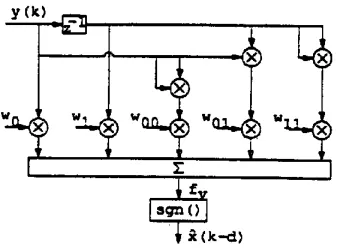
The coefficients w i, w O, wot, etc are known as the Volterra kernals.

In theory the number of terms in equation (8) can be infinite. However in practice only a finite number of terms can be implemented. Consider a simple VS equaliser where M = 2 and the polynomial expansion is truncated to degree-2 terms:

~(k - d) = sgn(woy(k) + wi y(k - 1) +

wo0y2(k) + w01 y ( k ) y ( k - 1 ) + wjl yZ(k - 1 )) (10)

Adaptive Systems 1 ! 3

[

x

Fig. 11 Volterra equaliser of order 2 and degree 2.

2 i (k) -~i

1

×

-2

I T I

-2 -I 0 1

y(k)

(a) Dashed curve: M L P equalise~.

A I

0

v

! !

~(k)-i

2 ~ (k) -~i

I

X

-i x / •

×

-2

I I ! t

-2 -i 0 1

y(k)

(b) Dashed curve: VS equaLiser.

l

0

v

).

! 1 R(k)=l

Fig. 12 Comparison of decision boundaries. Channel

H ( z ) = l + 0 . 5 z -I, solid curve: optimal decision boundary.

.2 in Figure 5 and equation (2), was 0.2, representing a signal to noise ratio (SNR) of approximately 8 dB. The MLP has a 2 - 9 - 5 - 1 configuration. That is, the observation vector y(k) has 2 elements corre- sponding to the two tap channel transfer function, the first hidden layer has 9 nodes, the second hidden layer has 5 nodes and the output layer has 1 node. The VS equaliser has a structure of order 2 and degree 3. The decision boundaries of these two non- linear equalisers, obtained after a training sequence of 300 samples, are compared with the optimal deci- sion boundary in Figure 12(a) and (b) respectively. Performance of the MLP and VS equalisers for more realistic channels and equaliser configurations have extensively been studied (Chen, 1990IEE; Gibson.

1991SP).

7. THE RADIAL BASIS FUNCTION NETWORK

In this section a third adaptive nonlinear structure, namely the radial basis function (RBF) network of Broombead, is described. The RBF network is ideal for equalisation application because it has an equiv- alent structure to the optimal Bayesian equalisation solution (Chen, 1993NN). The schematic of the RBF network is depicted in Figure 13. The overall response of the network can be summarised in the following equation:

n r

fAy(t)) = ]~ wi$; (l l)

i=1

f i e

= ~,

w,¢~[v(lO-

c,~l 2/p;)

o u t p u t l a y e r

×>

l a y e r

y(k) y (k-M+l)

Figure 12 illustrates the performance of the straight- forward MLP and VS equalisers when used to equalise a simple channel with transfer function

H(z)

114 Adaptive Systems

ci are the RBF centres which have the same dimen- sional as the input vector y(k), II'll denotes the Euclidean norm, P i are t h e positive constants known as the widths, and ¢(.) is the basis function. To use the RBF network for detecting the channel input

x ( k - d ) , t h e output of the network, f r , is passed through a decision slicer.

The relationship between the RBF network and the Bayesian equalisation solution, equation (6), can be given explicitly (Mulgrew, 1996). The number of centres, nr, is equal to that of the noise-free channel output vector ~, and ei are in fact these vectors. The weights w i are all known and they are the corre- sponding scaling factors of the conditional density functions in equation (6). The widths P i are con- trolled by the noise variance n 2, and are usually set at

Pi = 2¢r, 2, while ¢(.) is the noise probability density function which is usually Gaussian. When these con- ditions are met, the RBF network realizes precisely the Bayesian equalisation solution.

For the simple channel and the equaliser configura- tion given in Figure 13, 60 training samples were used to estimate the RBF centres based on the clus- tering scheme. The resulting RBF equaliser produces a decision boundary which is indistinguishable from the optimal Bayesian decision boundary. The bit error rate of the _,O~ptive RBF equaliser was further compared with that of the optimal Bayesian equaliser for the channel with impulse response H ( z ) = O. 3482 +0. 8704z -l + 0. 3482z -2 under a variety of SNR val- ues. The equaliser had a s~ucture of M = 4 and d = 1. The adaptive RBF equaliser used the least mean square algorithm to identify the channel model with a training sequence of 90 samples. The bit error rate curves of the adaptive RBF and Bayesian equalisers are depicted in Figure 14. The third error rate curve in Figure 14 was obtained by the Wiener filter which is the theoretical performance bound of the linear equaliser. From Figure 14, it is seen that the adaptive RBF equaliser realizes the optimal per- formance and is far superior to the linear equaliser.

To realize the optimal Bayesian solution using the RBF network, one thus needs to identify the cenlres or the noise-free channel output vectors. Cben (1993) conveniently achieved this using two alterna- tive schemes. The first method identifies the channel model using standard linear adaptive algorithm and then calculates the noise-free vectors from the gener- ation mechanism, H x(k), of equation (5). The sec- ond method estimates these vectors or centres directly using a supervised and unsupervised cluster- ing algorithms (Cben, 1993NN and 1993SP).

°l ' ! ' ~ I

[ ! w i e n e r ~e±J.te= o l

_~ I.. ... ~ . . . ~ . . . , . . ~ - . . ~ . . ~ . . , . ~ . . . ± . . . - 1

- 2

,,=I

- 6

5 I0 15 20 25

S i g n a l to N o i s e R a t i o (dB)

Callender(1994) has also compared the RBE MLP and VS equalisers and added distance classification techniques based on the Mahalanobis distance metric. The modified Mahalanobis (Callender, 1992) adds noise to the covariance update recursion to avoid con- vergence problems.

The intimate link between the RBF network and the Bayesian equaliser makes the RBF design an attrac- tive solution to equalisation problems. The perfor- mance of the RBF equaliser is superior to the MLP and VS equalisers and it needs a much shorter train- ing period than these other two nonlinear equalisers. Moreover the two adaptive schemes for the RBF equaliser are guaranteed to converge to the optimal Bayesian solution.

8. THE DECISION FEEDBACK EQUALISER

A powerful technique to improve equalisation perfor- mance is to use decision feedback (Qureshi). A generic decision feedback equaliser (DFE) is illus- trated in Figure 15, where M and n b are known as the feedforward and feedback orders respectively. This structure is obtained by expanding the equaliser input vector y(k) of Figure 5 to include the past detected symbols t b ( k - d ) = [ ~ ( k - d - 1)...~(k - d - nh)] r. The conventional DFE (Qureshi) is based on a linear filtering of the expanded equaliser input vector [yr (k) tr(k - d)] r.

Fig. 14 Performance on the fixed

H ( z ) = 0. 3482 + 0. 8704z -z + 0. 3482z °2.

Adaptive Systems. 115

tures given previously can then be applied to adap- tively implement this Bayesian solu~on.+ In particular.:, the RBF design has many advantage.< It provides a clear explanation of how decision feedback improves performance, as well as reducing the computational complexity.

Fig. 15 A generic decision feedback equaliser.

Figure 16 shows results on a 4 symbol quadrature amplitude modulated (4-QAM) system, comparing a conventional DFE detector, a Bayesian (i.e. RBF) DFE and a maximum likelihood Viterbi algorithm (MLVA) equaliser, with delays of 2 & 10 symbols. The Bayesian is superior to the conventional detector by 3 dB but the MLVA is best with longer delay of 10 on this stationary channel, as it is able to perform a more accurate channel estimate.

design using a simulated mobile radio nonstationary

(l~lLag) c h ~ | . ~ channel input x ( k ) is again 4~(~AM and the symbol rate is 300 lffIz. The trans- mission pulse has a raised-cosine characteristic with a rolloff factor of 0.5 and is split equally between the transmitter and receiver filters. A multipath Rayleigh fading channel is simulated with a Doppler frequency of 100 Hz, and the channel dispersion spans 4 sym- bol durations. The time-varying channel thus has a transfer function

H ( z ) = ho(k) + hm(k)z-l + . . . +h4(k)z -4 (12)

The time-varying taps hi(k) and the channel output

y( k ) are complex-valued.

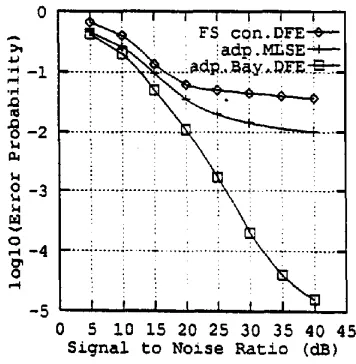
Three adaptive equalisers, namely the conventional DFE, the maximum likelihood sequence estimator (MLSE) (Forney) and the Bayesian DFE based on the RBF design, are investigated. The conventional DFE is fractional spaced (FS), that is, the channel output is sampled at a rate faster than the symbol rate. It has nine half-symbol spaced feedforward terms and 4 feedback terms. The MLSE is implemented as a Viterbi detector with a fixed decision delay of 6 sym- bol periods and equipped with a least mean square channel estimator. The Bayesian DFE based on the RBF design has a structure of d = 2, M = 3 and nb= 4, and it employs a least mean square channel estimator to adaptively update the RBF centres. The symbol error rates of these three adaptive equalisers are depicted in Figure 17.

0 !

con. det~.

-- ~ Bay. deti. t

~

-6 i

10 15 20 25 30

signal to Noise Ratio (dB)

Fig. 16 DFE performance comparisons on the same channel as used in Fig. 14.

Chert (1993SP) has also demonstrated adaptive per- formance of the Bayesian DFE based on the RBF

0

.,4

o _ ~

v O - * - 4

O

-5

! I I I I I I

~ - ~ 4 ~ : rs e o n . D F X

iiiiii!!i

...

i!i!i

...

!!ili

. - . - . . _

0 5 i0 15 20 25 30 35 40 45 S i g n a l to N o i s e P a t i o (dB)

Fig. 17 Performance comparison for a multipath fad- ing mobile radio channel with 100 Hz Doppler.

116 Adaptive Systems configurations of Figures 6 and 16 are known as the

symbol-by-symbol equaliser where detection of the channel input sequence is on a symbol-by-symbol basis. The MLSE on the other hand is the optimal solution for a very different class of sequence- estimation equalisers. It provides the lowest error rate attainable for any equaliser when the channel is known. However, for fast time-varying channels such as moble radio fading channels, the adaptive MLSE suffers serious performance degradation due to chan- nel tracking errors. In contrast the adaptive Bayesian DFE based on the RBF design is very robust and suf- fers a much smaller degradation in the time-varying environment. A more extensive simulation study is presented in (Chan, 1995).

It has also been convincingly demonstrated how the RBF can be deployed to realise new designs of blind equalisers with equally significant

performance

moid network model (Chen, 1990LIC; Weigend). Chen (1994JASE) has also fitted an RBF model to this sunspot time series.

Because this is a scalar time series, Chens (1994JASE) RBF network employed a single output node. The nonlinearity of hidden nodes was chosen to be the thin-plate-spline function. The desired value for the predictor lag was derived by fitting RBF predictors of different lags and choosing one that gives the best result. For the sunspot time series, it is found that a lag of 8 was an appropriate choice. The one-step RBF predictor

9(t + I I t)= f, (y(t), y(t - I),... y(t - 7)) (13) was fitted to the training data set. The evaluation of the fitted R B F predictor is then done by examining

the prediction error and the normalized prediction variance was further used to evaluate the fitted RBF model.

9. SIGNAL PREDICTION

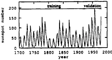
These nonlinear processing techniques are equally applicable to signal prediction (Mulgrew, 1992) and system modelling (Cben, 1992IJC) as well as equali- sation. Application of the RBF model to nonlinear signal prediction has been regularly demonstrated by analyzing for example the time series of the annual sunspot numbers. The annual sunspot numbers for the years 1700-1979 are plotted as 280 observations in Figure 18.

2 0 0

150 c

i00

~ 5o 0 1700

' =tu~--~' ' ' vLlidaUon

1750 1800 1850 1900 1950 year

I000

Fig. 18 Sun spot time series data.

The sunspot data from 1700 to 1920 were used for training and the data from 1921 to 1979 were employed for evaluating predictive accuracy. Because this time series is nonstationery, a shorter v~flidation set, 1921-1955, is also used for evaluation of the prediction accuracy. Many researchers have fitted various predictors or models to the sunspot time series. These include the linear autoregressive model and the bilinear model (Gabr), the threshold autore- gressive model (Tong), the polynomial or Volterra- series (Cben, 1989), and the one-hidden-layer sig-

c o

-*-4

200

®

~q

.Q 0 1 5 0

1 0 0

~ 5o

g o

! 1 ! ! !

o b s e r v a t i o n .4)-- p r e d i c t i o n -+--

+

I I

1 9 2 0 1 9 3 0 1 9 4 0 1 9 5 0 1 9 6 0 1 9 7 0 1 9 8 0 y e a r

Fig. 19 RBF predictor fitted to Fig. 18 validation data with the OLS training algorithm.

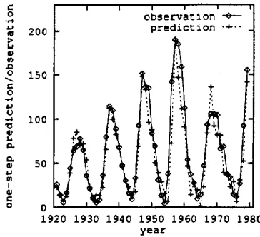
The training set has 221 samples and therefore there are 221 candidates for the RBF centres. The orthog- onal least squares (OLS) algorithm was initially employed to construct a one-step RBF predictor. As expected, when the OLS algorithm added more cen- tres to the selected RBF network, the accuracy of the model over the training set continued to improve. After 25 centres had been selected, the normalised variance over the validation set began to increase as more centres were added in to the network. This sug- gested that the selection procedure should be termi- nated at the 25th step, giving rise to a RBF predictor of 25 centres. Figure 19 shows the one-step predic- tions over the validation set, superimposed on the time series observations.

Adaptive Systen~s 117

sunspot time series (Chen 1994JASE). The number of hidden nodes was again chosen to be 25: ' The training input data were passed through the clustering algorithm five times with the corresponding adaptive gain being 0.2, 0.1, 0.05, 0.025 and 0.01. After the centres had been obtained, the weights were then learnt using the recusive least squares (RLS) algo- rithm. Repeated training was performed by passing the data through the RLS algorithm five times. The one-step predictions over the years 1921-1979 are again superimposed on the original time series obser- vations in Figure 20. Comparing Figure 19 with Fig- ure 18, it can be seen that the predictor obtained by the OLS algorithm has better short-term predictions than the predictor fitted by the clustering and RLS algorithm, but the long-term predictions of the latter are better than those of the former!

the RBF network.

10. CONCLUSIONS

This paper has attempted to briefly review the appli- cation of nonlinear filter structures to noise reduction, channel equalisation and prediction problems. These sffuctures show considerable promise for improved noise reduction and the nonlinear adaptive filters give significantly improved equaliser performance over linear filter approaches. Recent equaliser research has focused on the radial basis function design incorpo- rating decision feedback, and this provides a practical and powerful equalisation scheme which even outper- forms the maximum likelihood sequence-detection in a highly nonstationary environment.

t - o

L ,

.D

O

O

D~

r .

o 2 0 0

150

100

50

I i i

o b s e r v a t i o n p r e d i c t i o n -÷--

0

1920 1930 1940 1950 1960 1970 1980 y e a r

Fig. 20 R B F predictor fitted to Fig. 18 validation data with clustering and the R L S algorithm.

Some time ago Chen (1989) fitted a subset polyno- mial model to the sunspot time series and showed that it had better performance than the linear and bilinear models of Gabr. For the sake of comparison, Chen selected the same predictor lag of 9 as used in the linear and bilinear models. Weigend has also constructed a sigmoid network model for the sunspot time series and demonstrated its superior perfor- mance over the threshold model of Tong. They chose a predictor lag of 12 because this was the value used in the threshold model. The overall multi-step pre- diction performance of the RBF model obtained in Cherts (1994JASE) study was better than either those of the subset polynomial model or the sigmoid net- work model. It is worth pointing out that only a modest number of cenues were used in the Chen RBF model. Weigend surprisingly commented that the RBF approach was inefficient and required a very large number of centres. Chens more recent results clearly suggest otherwise! Chen (1994JASE) also describes other system modelling simulations using

The results presented here are typical of those received from nonlinear filter designs, and hence the RBF is now assuming a prominant position as one of the most am'active nonlinear filter design approaches. As a result of these excellent results the RBF is now being applied to other communications processor functions such as interference cancellation (Mulgrew,

1995) and bearing estimation.

11. ACKNOWLEDGEMENTS

This paper is one of a continuously developing series on nonlinear filtering. The authors wish to thank par- ticularly Sbeng Chen for access to his recent research results. We also wish to acknowledge the significant contributions of Steve McLaughlin, Colin Cowan and Gavin Gibson to the work reviewed in this paper. The sponsorship of the UK Engineering and Physical Science Research Council under previous contracts GR/E/10357 and GR/FJ72380 is gratefully acknowl- edged.

12. REFERENCES

D.S. Bmomhead and D. Lowe, "Multivariable func- tional interpolation and adaptive networks," Complex Systems, Vol.2, pp.321-355, 1988.

C.P. Callender and C.F.N. Cowan, "Use of cluster classification for channel equalisation at high SNR",

IMA Mathematics in Signal Processing Conference Proceedings, Warwick, December 1992.

C.P. Callender and C.EN. Cowan, "A comparison of 6 different nonlinear equaliser techniques for digital communications systems", Proceedings Vll Euro. pean Signal Processing Conference, EUSIPCO-94, pp. 1524-1527, Edinburgh, Sept 1994.

I 18 Adaptive Systems ral networks", IEEE Int. Symposium Circuits and

Systems, pp. 995-998, May 1989.

S. Chen and S.A. Billings, "Modelling and analysis of non-linear time series", Int. Journal Control, Vol. 50, No. 6, pp. 2151-2171, 1989.

S. Chen, S.A. Billings and P.M. Grant, "Non-linear systems identification using neural networks", Int. Journal Control, Vol. 51, No. 6, pp. 1191-1214,

1990.

S. Chen, G.J. Gibson and C.EN. Cowan, "Adaptive channel equalisation using a polynomial-perceptron structure," IEE Proceedings, Part.l, Vo1.137, No.5, pp.257-264, 1990.

S. Chen and S.A. Billings, "Neural networks for non- linear dynamic system modelling and identification," Int. Journal Control, Special Issue on Intelligent Control, Vol.56, No.2, pp.319-346, 1992.

S. Chert, B. Mulgrew and P.M. Grant, "A clustering technique for digital communications channel equaii- sation using radial basis function networks," IEEE Trans. Neural Networks, Vol. 4, No. 4, pp. 570-579, July 1993.

S. Chen, B. Mulgrew and S. McLaugblin, "Adaptive Bayesian equaliser with decision feedback," IEEE Trans. Signal Processing, Vol. 41, No. 9, pp. 2918-2926, 1993.

S. Chen, "Radial basis functions for signal prediction and system modelling", Journal of Applied Science & Engineering, Vol. I, No. 1, June 1994.

S. Chen, S. McLaughlin, B. Mulgrew and P.M. Grant, "Adaptive Bayesian decision f~dback equaliser incorperating cochannel interference suppression", in proceedings IEEE Int. Conference Communications, Vol. 1, pp. 530-533, May 1994.

S. Chen, S. McLaughlin, B. Mulgrew and P.M. Grant, "Adaptive Bayesian decision feedback equaliser for dispersive mobile radio channels," IEEE Trans. Com- munications, Vol.43, No.5, pp.1937-1946, May 1995. G.D. Forney, "Maximum-likelihood sequence estima- tion of digital sequences in the presence of intersym- bol interference," IEEE Trans. Information Theory, VoI,IT-18, No.3, pp.363-378, 1972.

M. Gabbouj, EJ. Coyle and N.C. Gallacher "An Overview of median and stack filters", Circuits, Sys- tems Signal Processing, Vol. 1 I, No. I, pp. 7-45, 1992.

M.M. Gabr and T. Subba Rao, "The estimation and prediction of subset bilinear time series models with applications", Journal Time Series Analysis, Vol. 2, pp. 155-171,

G.J. Gibson and C.EN. Cowan, "On the decision

region of multi-layer pcrceptrons," Proc. IEEE, Vol.78, No.10, pp.1590-1594, 1990.

G.J. Gibson, S. Siu and C.F.N. Cowan, "The applica- tion of nonlinear structures to the reconstruction of binary signals," IEEE Trans. Signal Processing, Vol.39, No.8, pp.1877-1884, 1991.

C.Z.W. Hassell Sweatman, G.J. Gibson and B. Mul- grew, "A Constructive Algorithm for Neural Network Design and Application to Channel Equalization", IMA Conference on Applications of Combinatorial Mathematics, December 1994.

R.P. Lippmann, "An introduction to computing with neural nets," IEEE ASSP Magazine, Vol.4, pp.4-21, 1987.

W.S. McCuiloch and W. Pitts, "A Logical Calculus of the Ideas Imminent in Nervous Activity", Bulletin on Mathematical Biophysics Vol. 5, pp. 115-133, 1943. B. Mulgrew, K. Nisbet and S. McLaughlin, "Degen- eracy of nonlinear predictor," in Proc. VI European Signal Processing Conference, EUSLPCO-92, Brus- sels, 1992, pp.791-794.

B. Mulgrew, E.S. Warner and P.M. Grant, "A Bayesian receiver for asynchronous CDMA commu- nications", in IEEE PIMRC Conference Proceedings pp. 985-989, September 1995.

B. Mulgrew, "Applying Radial Basis Functions", IEEE Signal Processing Magazine, Vol. 13, No. 2, pp. 50-65, March 1996.

S.U.H. Qureshi, "Adaptive equalization," Proc. IEEE, Vol.73, No.9, pp.1349-1387, 1985.

D.E. Rumelhart, G.E. Hinton and R.J. Williams, "Learning internal representations by error propaga- tion," in Parallel Distributed Processing: Explo- rations in the Microstructure of Cognition, D.E. Rumelhart and J.L. McCldland, Eds., Cambridge, MA: M1T Press, 1986, pp.318-362.

I. Tabus, M. Gabbouj and L. Lin, "Real domain adap- tive WOS filtering using neural network approxima- tions", IEEE Winter Workshop on Nonlinear DSP, pp. 7.2-1.1 to 7.2--1.6, Jan 1993.

H. Tong and K.S. Lira, "Threshold autoregression, limit cycles and cyclical data", Journal Royal Statisti- cal Society, B Vol. 42, pp. 245-292, 1980.

A.S. Weigend, B.A. Huberman and D.E. Rumelhart, "Predicting the future: a connectionist approach", Int. Journal Neural Systems, Vol. 1, No. 3, pp. 193-209,

1990.

L. Yin, J. Astola and Y. Neuvo, "Adaptive stack filter- ing with application to image processing", IEEE