University of Southampton Research Repository
ePrints Soton
Copyright © and Moral Rights for this thesis are retained by the author and/or other
copyright owners. A copy can be downloaded for personal non-commercial
research or study, without prior permission or charge. This thesis cannot be
reproduced or quoted extensively from without first obtaining permission in writing
from the copyright holder/s. The content must not be changed in any way or sold
commercially in any format or medium without the formal permission of the
copyright holders.
When referring to this work, full bibliographic details including the author, title,
awarding institution and date of the thesis must be given e.g.
AUTHOR (year of submission) "Full thesis title", University of Southampton, name
of the University School or Department, PhD Thesis, pagination
MODELLING GENETIC ALGORITHMS
AND EVOLVING POPULATIONS
By
Alexander Rogers B.Sc.(Hons)
A thesis submitted for the degree of Doctor of Philosophy
Department of Electronics and Computer Science University of Southampton
United Kingdom
UNIVERSITY OF SOUTHAMPTON
ABSTRACT
FACULTY OF ENGINEERING
ELECTRONICS AND COMPUTER SCIENCE DEPARTMENT
Doctor of Philosophy
Modelling Genetic Algorithms and Evolving Populations
by Alexander Rogers
A formalism for modelling the dynamics of genetic algorithms using methods from statistical physics, originally due to Pr¨ugel-Bennett and Shapiro, is extended to ranking selection, a form of selection commonly used in the genetic algorithm com-munity. The extension allows a reduction in the number of macroscopic variables required to model the mean behaviour of the genetic algorithm. This reduction allows a more qualitative understanding of the dynamics to be developed without sacrificing quantitative accuracy.
The work is extended beyond modelling the dynamics of the genetic algorithm. A caricature of an optimisation problem with many local minima is considered — the basin with a barrier problem. The first passage time — the time required to escape the local minima to the global minimum — is calculated and insights gained as to how the genetic algorithm is searching the landscape. The interaction of the various genetic algorithm operators and how these interactions give rise to optimal parameters values is studied.
Contents
Declaration x
Acknowledgements xi
Chapter 1 Introduction 1
1.1 The Genetic Algorithm . . . 1
1.2 Genetic Algorithm Theory and Modelling . . . 2
1.2.1 Microscopic models . . . 4
1.2.2 Macroscopic models . . . 4
1.2.3 Biological models . . . 5
1.3 Thesis Goal . . . 6
1.4 Thesis Outline . . . 7
Chapter 2 Statistical Physics Formalism 9 2.1 Introduction . . . 9
2.2 Generational Selection . . . 9
2.2.1 The Model Genetic Algorithm . . . 9
2.2.2 Selection . . . 10
2.2.3 Integrating around a Gaussian . . . 12
2.2.4 Finite Sample Effects . . . 12
2.2.5 Weak Selection Expansion . . . 13
2.2.6 Mean Behaviour . . . 14
2.3 Steady State Selection . . . 15
2.3.1 Calculating Selection . . . 15
2.3.2 Strong Selection . . . 16
2.3.3 Weak Selection . . . 17
2.3.4 Small Beta Expansion . . . 19
2.3.5 Comparison with Simulation Data . . . 19
2.4 Comparison of Generational and Steady State GA . . . 20
2.5 Discussion . . . 22
Chapter 3 Genetic Drift in Selection Schemes 25 3.1 Introduction . . . 25
3.2 Population Fitness Variance . . . 26
3.3 Results . . . 28
3.4 Performing the Calculations . . . 30
3.4.1 Generational Selection . . . 30
3.4.2 Steady State Selection . . . 31
3.4.3 Varying Generation Gap . . . 31
3.4.4 CHC Algorithm . . . 32
3.5 Evolutionary Strategies . . . 33
3.6 Discussion . . . 35
Chapter 4 Ranking Selection 38 4.1 Introduction . . . 38
4.2 Ranking Selection . . . 39
4.2.1 Infinite Population Model . . . 40
4.2.2 Tournament Selection . . . 41
4.2.3 Finite Population Effects . . . 41
4.2.4 Roulette Wheel and Stochastic Universal Sampling . . . 42
4.3 Results . . . 45
4.4 Discussion . . . 46
Chapter 5 Crossover and the Onemax Problem 48 5.1 Introduction . . . 48
5.2 Onemax . . . 48
5.2.1 The Model Genetic Algorithm . . . 49
5.2.2 Selection . . . 49
5.2.3 Mutation . . . 50
5.2.4 Crossover . . . 50
5.3 Results . . . 54
5.4 The Original Interpretation ofC . . . 54
5.5 Linkage Equilibrium and a Closed Form Approximation . . . 57
5.6 Discussion . . . 60
Chapter 6 Stabilising Selection 61 6.1 Introduction . . . 61
6.2 Stabilising Selection . . . 63
6.3 Results . . . 65
6.4 Equilibrium Distribution . . . 65
6.5 A Closed Form Solution . . . 68
6.6 Discussion . . . 70
Chapter 7 Solving the Basin with a Barrier 72 7.1 Introduction . . . 72
7.2 First Passage Time . . . 73
7.3 Simulation Results . . . 74
7.4 Theoretical Analysis . . . 75
7.4.1 Population Size . . . 76
7.4.2 Selection Scheme . . . 77
7.4.3 Mutation Rate . . . 77
7.4.4 String Length . . . 79
7.5 Stochastic Walker . . . 80
7.6 Conclusions . . . 81
Chapter 8 Biological Models 82 8.1 Introduction . . . 82
8.2 Overlapping and Non-Overlapping Generations . . . 82
8.3 Stabilising Selection-Mutation Balance . . . 84
8.3.1 Mutation Rate Threshold . . . 86
8.4 Discussion . . . 87
Chapter 9 Conclusions and Future Directions 89 9.1 Introduction . . . 89
9.2 Low Mutation Phase Transition . . . 89
9.3 Conclusions . . . 92
Appendix A Mutation 93
Appendix B Crossover 95
Appendix C Correlation under Selection 97
Appendix D Linkage Equilibrium 100
Appendix E Stabilising Selection 102
Appendix F First Passage Time 104
Bibliography 105
List of Figures
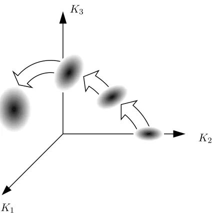
2.1 Ensemble of populations evolving in the phase space of macroscopic variables. . . 14
2.2 Strong and weak selection comparison. . . 18
2.3 Comparison of simulation and theory for steady state selection. . . 20
2.4 Comparison of simulation data for generational and steady state se-lection. . . 22
2.5 Comparison of simulation data for generational and steady state ge-netic algorithms with rescaled parameters. . . 23
3.1 Comparison of the rate of genetic drift. . . 29
3.2 Comparison of the rate of genetic drift in evolutionary strategies. . 34
3.3 Comparison of genetic algorithm selection schemes. . . 36
4.1 Comparison of simulation and theory calculation of finite population effects for roulette wheel selection. . . 43
4.2 Comparison of simulation and theory calculation ofhn2i for
stochas-tic universal sampling. . . 44
4.3 Comparison of finite population effects for roulette wheel selection and stochastic universal sampling. . . 45
4.4 Comparison of theory and simulation for finite population effects with roulette wheel selection. . . 46
4.5 Comparison of theory and simulation for finite population effects with stochastic universal sampling. . . 47
5.1 Diagram of deviation from natural correlation. . . 52
5.2 Comparison forC for roulette wheel selection and stochastic univer-sal sampling. . . 53
5.3 Simulation and theoretical results for onemax. . . 55
5.4 Comparison of theoretical and simulation results for the C within the population. . . 56
5.5 Comparison of numerical and simulation results for the end point equilibrium of onemax. . . 58
5.6 Comparison of numerical and analytical theory results for the end point equilibrium of onemax. . . 59
6.1 The basin with a barrier problem. . . 62
6.2 Simulation and theory results for the basin with a barrier problem. 66
6.3 Comparison of theoretical numerical solutions and simulation results for the end point equilibrium for the basin with a barrier with crossover. 67
6.4 Comparison of theoretical numerical solutions and simulation results for the end point equilibrium for the basin with a barrier without crossover. . . 67
6.5 Comparison of theoretical numerical solutions and closed form ex-pressions for end point equilibrium for the basin with a barrier with crossover. . . 71
6.6 Comparison of theoretical numerical solutions and closed form ex-pressions for end point equilibrium for the basin with a barrier with-out crossover. . . 71
7.1 Simulation of time to solve the basin with a barrier problem. . . 74
7.2 Theoretical calculation of time to solve the basin with a barrier problem 75
7.3 Comparison of finite population effect for roulette wheel selection and stochastic universal sampling. . . 76
7.4 Changing population size in the basin with a barrier problem. . . . 78
7.5 Changing string length in the basin with a barrier problem. . . 79
7.6 Theoretical first passage times for a single stochastic walker to solve the basin with a barrier. . . 80
8.1 Comparison of simulation and theory results for equilibrium mean and variance for sexual and asexual populations in stabilising selec-tion - mutaselec-tion balance. . . 85
8.2 Comparison of mutation rate threshold in sexual and asexual popu-lations with changing loci number. . . 87
9.1 Simulation results of equilibrium variance at the low mutation thresh-old in stabilising selection. . . 90
9.2 Simulation results showing phase transition in correlation under sta-bilising selection. . . 91
Declaration
No portion of the work referred to in this thesis has been submitted in support of an application for another degree or qualification of this or any other university or other institution of learning.
Acknowledgements
I would like to thank Adam Pr¨ugel-Bennett for providing direction and supervision throughout the course of this research and for not solving all the problems himself. I would also like to thank Neil Lawrence and Bart Naudts for many useful discussions and Margaret Ann and Eleanor Mary for providing diversion.
I gratefully acknowledge a research studentship awarded by the Engineering and Physical Sciences Research Council (ref. 97307210).
Chapter 1
Introduction
1.1 The Genetic Algorithm
The genetic algorithm (GA) came to popularity through the work of John Holland [11] in 1975. It is now commonly seen as a generic stochastic search algorithm and as such is often applied to combinatorial optimisation problems. These problems generally exhibit un-characterised problem spaces which are highly dimensional and have many local minima; features which prevent the use of traditional optimisation techniques.
At its simplest the genetic algorithm functions as a simple model of an evolving population. Potential solutions to the problem under study are mapped onto a binary string which represents the genetic material of the individual. A population of such individuals is maintained and allowed to evolve in a caricature of natural evolution. A cost function maps the encoded solution to a fitness value on which selection acts: replicating fitter individuals and culling the less fit. Mutation acts to generate small changes in the genetic code of each individual and recombination or crossover allows individuals to exchange genetic material. By repeating this process, it is hoped that good solutions to the problem are evolved.
Genetic algorithms operate in the realm of stochastic search operators and compete with more established techniques such as the Metropolis algorithm [17] or simulated annealing [14]. In these algorithms, the problem is again represented in a form which allows local moves to be generated. If only moves which improve fitness are accepted, the algorithms rapidly become trapped in local minima. To avoid this, the Metropolis algorithm allows moves which are detrimental to fitness with some
1.2. GENETIC ALGORITHM THEORY AND MODELLING 2 small probability. The probability of these moves is controlled by a temperature parameter. If the criteria for accepting moves is chosen correctly, the algorithm asymptotically samples according to the Gibbs distribution.
If the temperature is low and the system is in equilibrium, there is a high probability of sampling the global minimum. One difficulty of this approach is that at low temperature, reaching equilibrium can be very slow. Simulated annealing remedies this by allowing a gradual lowering of the temperature – annealing. If done slowly, so that the system remains in equilibrium, the algorithm is shown to converge to the global minimum. In practice, such time scales are not available and the algorithm eventually freezes into a local minimum. Choosing the annealing schedule is critical to the success of any simulated annealing algorithm.
The genetic algorithm is differentiated from these stochastic search methods by the maintenance of a population and the possibility of performing recombination. In the common understanding of the genetic algorithm, the population of individuals, performing local search through mutation, allows the algorithm to escape local minima. Crossover allows moves on the landscape which are more global in nature, potentially finding new fitter areas for further search. Whilst there is no single parameter such as temperature, it is clear that the dynamics of the genetic algorithm are parameterised indirectly through the choice of selection scheme, mutation rate and crossover.
Understanding the interplay of these various parameters is a very complex problem and little progress has been made. Yet without some theoretical basis, practitioners are forced to work by a set of ‘rules of thumb’ which have been shown to work on previous problems. There is a clear need for a comprehensive theory which would give some insight into the sort of problems where genetic algorithms should excel and gives some guidance as to how to set the various parameters.
1.2 Genetic Algorithm Theory and Modelling
1.2. GENETIC ALGORITHM THEORY AND MODELLING 3 Much of the genetic algorithm theory literature is still based around the schema theory and it has received renewed interest recently through the work of Stephens [44]. The original problems remain despite being reformulated. It results in an inequality for the probability of occurrence of each schema in the next generation, if the average fitness of each schema in the current generation is known. It is thus not able to predict the dynamics of the evolving population and it is unclear how the schema theorem will help understanding of genetic algorithms.
A less expansive approach is to try to develop a simple model of the genetic al-gorithm. Rather than attempting to make general comments on a broad range of algorithms and problems, the details of a number of simple cases may be studied to try to develop an insight into how the genetic algorithm is working. To be of use, such a model must capture the essential elements of the genetic algorithm but not become so complex that the underlying process is obscured by the details. Creating such a model is difficult for a number of reasons:
- The problem size is extremely large. For a binary string of typical length 100, there are 2100 possible genotypes or binary combinations.
- The small population sizes of typically 100 individuals, sample a very small fraction of the total search space. Thus theoretical results based on infinite population models are often misleading. Indeed much of the interesting phe-nomena observed in the evolution of genetic algorithms are features of a finite population.
- The translation from the encoding of the binary string to a fitness value for any particular individual is often highly non-linear and simple cases need to be studied to make any real progress.
- The interaction between population members in terms of the selection of fitter members and the transfer of genetic material between them in crossover is fundamental to the power of the genetic algorithm. It is thus not possible to model an average population member and the entire population of interacting individuals must be modelled.
1.2. GENETIC ALGORITHM THEORY AND MODELLING 4
1.2.1 Microscopic models
The evolution of a genetic algorithm from one generation to another is simply subject to the influence of selection, mutation and crossover. If at each generation, the population can be exactly described, the resulting evolution may be described by a Markov chain. This approach has been pioneered by Vose and collaborators [50, 51, 27, 53] and is detailed in Vose’s recent book [52].
Such models consider all the microscopic detail of the population and construct transition matrices which describe the change in the population due to the various genetic operators. To describe problems of reasonable size, very large matrices are generated and in general, these may only be solved in the infinite population limit.
Relating infinite population results back to the finite population case must be done carefully and it is here that the microscopic models encounter difficulties. The state space of the genetic algorithm is vast compared to the typical size of population used. Thus the response of an infinite population can be very different from that of the finite population under analysis and many of the interesting features of the genetic algorithm relate to the existence of a finite population.
1.2.2 Macroscopic models
Whilst analysis of the population at the microscopic level can be exact, it is often not what is of interest. Macroscopic descriptions such as the average fitness of the population or the fittest member of the population tend to be more useful in gaining a qualitative understanding of what is happening.
This situation is similar to that in physics when modelling the properties of a material. The behaviour and state of every individual atom contributes to the bulk properties of the material such its magnetism or temperature. However it is these bulk properties which are of interest and much can be said about the behaviour of the material without having to worry about the microscopic details. For example, thermodynamics allows the behaviour of gases to be predicted without resorting to a calculation of the velocity of every molecule.
1.2. GENETIC ALGORITHM THEORY AND MODELLING 5 Crutchfield and Van Nimvegen at the Santa Fe Institute have taken this approach [49, 48]. By starting at the level of the transition matrices and extracting the macro-scopic descriptors which are of interest, they have been able to model the dynamics of a simple genetic algorithm on the royal road functions [18]. Unfortunately in-cluding crossover into their formalism has proved to be very difficult. Whilst this does not prevent the analysis of problems such as the royal road function, where crossover is shown to be of little benefit, it limits the applicability to other problem spaces.
Another approach to the macroscopic modelling of the genetic algorithm is to start with a macroscopic description of the population, or more precisely its fitness distri-bution, and model the effect of selection. Theile and Blickle [3] compared selection schemes by considering the mean and variance of fitness in an infinite population and M¨uhlenbein [26, 23, 24] modeled a special class of genetic algorithm using a similar technique. In general, the accuracy of these models precluded them from considering more that one generation and they gave qualitative results rather then quantitative predictions of the dynamics of a genetic algorithm.
The formalism developed by Pr¨ugel-Bennett and Shapiro [29, 43, 41, 30, 42] and later extended by Rattray [32] represents the most sophisticated of these approaches. The population fitness distribution is described by its cumulants and finite popula-tion effects are calculated accurately. The accuracy of the model allows the calcu-lations for one generation to be iterated and the dynamics of the genetic algorithm followed over many generations. Significantly, not only is selection considered but the formalism is extended to mutation and crossover. This allows the dynamics of a simple genetic algorithm to be completely modelled on a number of simple problems. It is this formalism which provides the basis for the work in this thesis.
1.2.3 Biological models
For obvious reasons many of the simple models of genetic algorithms are very similar to biological models of evolving populations. The field of quantitative genetics is much more established than that of genetic algorithms with the work of Fisher [10] and Wright [54] dating back to the nineteen twenties and thirties.
1.3. THESIS GOAL 6 and thus the models concentrate on the particular allele frequency at each loci; equivalent to considering the individual probabilities that each bit is either a one or zero.
Despite this difference in focus, models of evolving populations which now appear to be very similar to simple models of genetic algorithms have been proposed by many researchers, amongst them Moran [21, 20, 19] and Kimura [13]. Typically these are solved by making a diffusion equation approximation to the Markov chain analysis; a technique which is of direct use in the microscopic modeling of genetic algorithms.
1.3 Thesis Goal
The aim of modelling the genetic algorithm is to gain insight into how the algorithm works. Genetic algorithms are complex systems and to model them a number of simple cases must be considered. The aim is always to reduce the complexity of the model without removing the fundamental features which are of interest. By studying these simple cases, techniques and insights are gained which will hopefully be of use to other more complex cases.
The formalism developed by Pr¨ugel-Bennett and Shapiro and later extended by Rattray has been applied to a range of simple cases by these researchers. Due to the complexities involved, much of the focus of the work so far has been in deriving the formalism. Whilst being quantitatively accurate, the model developed is not particularly amenable to qualitative analysis.
In this thesis, the formalism is extended to a more common form of selection scheme and in the process, significantly simplified. This simplification reduces the number of macroscopic variables required to describe the genetic algorithm and allows a more qualitative understanding of the dynamics to be developed without sacrificing quantitative accuracy.
1.4. THESIS OUTLINE 7 The work presented in this thesis has previously been published in a number of sources [35, 34, 37, 39, 36, 38].
1.4 Thesis Outline
The thesis is presented as detailed below:
• Chapter 2 - Statistical Physics Formalism
The formalism developed by Pr¨ugel-Bennett and Shapiro is presented and extended to the case of steady state genetic algorithms.
• Chapter 3 - Genetic Drift in Selection Schemes
The comparison of genetic drift in selection schemes is generalised by devel-oping a simple method of calculating the rate of genetic drift. The technique is applied to a range of genetic algorithm selection schemes and those used in evolutionary strategies.
• Chapter 4 - Ranking Selection
The formalism originally developed by Pr¨ugel-Bennett and Shapiro is ex-tended to the case of ranking selection. Finite population effects for both roulette wheel and stochastic universal sampling are calculated and compared. • Chapter 5 - Crossover and the Onemax Problem
The dynamics of a full genetic algorithm under selection, mutation and crossover is modelled on the onemax problem. Closed form expressions are derived for the equilibrium point.
• Chapter 6 - Stabilising Selection
A model of a hard optimisation problem – the basin with a barrier problem – is introduced and the analysis of ranking selection is extended to the case of stabilising selection in order to model the dynamics of the genetic algorithm on this problem.
• Chapter 7 - Solving the Basin with a Barrier
The analysis of stabilising selection is used to calculate the time to solve the basin with a barrier problem. The influence of the genetic algorithm parameters – population size, mutation rate and selection scheme – on this time are explored.
• Chapter 8 - Biological Models
1.4. THESIS OUTLINE 8 • Chapter 9 - Conclusions and Future Directions
Chapter 2
Statistical Physics Formalism
2.1 Introduction
The formalism developed by Pr¨ugel-Bennett and Shapiro [29, 43, 41, 30, 42] and later extended by Rattray [32] allows the dynamics of a simple genetic algorithm to be modelled. It is based on a macroscopic description of the population fit-ness distribution using the cumulants of the distribution. Selection is modelled by calculating the effect on these cumulants.
The formalism was initially developed considering generational Boltzmann selection and is presented first in this form. The value of the formalism for exploring questions of interest in the genetic algorithm community is demonstrated by extending it to the case of steady state selection. This work represents the first formal comparison of the two schemes – previous analysis being based on empirical observations.
2.2 Generational Selection
In the generational or canonical genetic algorithm, selection is applied once to an initial population, generating a new population of P individuals. As selection operates solely on the fitness of individuals within the population, a population with discrete fitnesses can be considered without initially having to consider the details of any particular problem space or encoding.
2.2.1 The Model Genetic Algorithm
The model genetic algorithm considered consists of a population of P individuals each with some assigned fitness value, F. At each time generation, Boltzmann
2.2. GENERATIONAL SELECTION 10 roulette wheel selection is performed whereby P population members are drawn independently with replacement from the original population using the weighting
wα =
eβFα
Z (2.1)
where β is a parameter allowing control of the selection strength and Z is the normalisation factor over the population
Z =
P
X
α=1
eβFα (2.2)
commonly referred to as the partition function.
2.2.2 Selection
The macroscopic variables chosen to model the fitness distribution are the distribu-tion cumulants, denoted byKn. These are natural variables to describe distributions
close to a Gaussian. The first two cumulants are familiar as the mean and vari-ance. Higher order cumulants describe the deviation away from a Gaussian - the third and fourth being related to the skewness and kurtosis. Unlike distribution moments, cumulants are invariant under a change of mean.
The cumulants of any continuous distribution, ρ(F), may be calculated from the cumulant generating function
Kn =
dn
dznG(z)|z=0 (2.3)
where
G(z) = log µZ
ρ(F) ezFdF
. (2.4)
2.2. GENERATIONAL SELECTION 11 The generating function for the ensemble distribution is thus given by the average over the weighted finite population
G(z) = *
log à P
X
α=1
wαezFα
!+
(2.5)
where the angle brackets denote averaging over all ways of sampling a finite popula-tion from the ensemble probability distribupopula-tion and all ways of performing selecpopula-tion on that finite population. Using the Boltzmann weighting from equation (2.1) allows the logarithm to be expanded
log à P
X
α=1
wαezFα
!
= log à P
X
α=1
eβFαezFα
!
−log à P
X
α=1
eβFα
!
. (2.6)
The second term does not depend on z and can thus be neglected. Changing variables gives
G(β) = *
log à P
X
α=1
eβFα
!+
(2.7)
where the cumulants after selection are now given by
Kn=
dn
dβnG(β). (2.8)
To evaluate equation (2.7), Pr¨ugel-Bennett and Shapiro took a technique from statistical physics used by Derrida to solve the random energy model [7]. The logarithm is represented as
log (Z) = Z ∞
0
e−t−e−tZ
t dt. (2.9)
The generating function thus becomes
G(β) = Z ∞
0
e−t−gP (t, β)
t dt (2.10)
where
g(t, β) = Z
ρ(F) e−teβFdF (2.11)
2.2. GENERATIONAL SELECTION 12
2.2.3 Integrating around a Gaussian
The generating function derived above may be evaluated numerically assuming the ensemble fitness distribution, ρ(F), can be described in terms of its initial cumulants. A convenient form is an expansion around a Gaussian using the Gram-Charlier expansion
ρ(F) = √ 1 2πK2
exp Ã
−(F −K1)2
2K2
! "
1 +
n
X
i=3
Ki
i!K2i/2Hi
µ
F −K1
√
K2
¶#
where Hi(x) are Hermite polynomials
Hi(x) = (−1)ie
x2 2 d
i
dxi
³ e−x22
´
(2.12)
andn is the number of cumulants used. Whilst the resulting distribution is close to a Gaussian and has the correct cumulants, it can be negative in places and is thus an approximation to the correct probability distribution.
Whennis two, the expansion has exactly the form of a Gaussian. Adding in further terms distorts the Gaussian to give the desired distribution. The first two terms expanded out are
H3(x) = x3−3x
H4(x) = x4−6x2+ 3. (2.13)
To fully describe the distribution, an infinite number of cumulants are required. In general, a truncated set may be used to give quantitatively good results. Pr¨ ugel-Bennett and Shapiro found that four cumulants were normally sufficient but cal-culating up to eight was sometimes necessary to generate quantitative agreement with simulation results.
2.2.4 Finite Sample Effects
Evaluating equation (2.10) and (2.11) using the Gram-Charlier expansion gives the cumulants of the ensemble, Kn, after selection. This includes the stochastic
effects which arise through selection operating on a finite population. However the cumulants of any finite population drawn from the ensemble,κn, will differ slightly
2.2. GENERATIONAL SELECTION 13 The cumulants of a finite population drawn from the ensemble may be found from the identities
κ1 = K1
κ2 = P2K2
κ3 = P3K3
κ4 = P4K4−6P2(K2)2/P (2.14)
where P2 =
¡ 1− 1
P
¢
, P3 = P2
¡ 1− 2
P
¢
and P4 = P2
¡ 1− 6
P + 6 P2
¢
. Here Kn
represents the cumulants of the continuous probability distribution and κn are the
cumulants of a finite population sampled from it. These results were originally shown by Fisher [10].
2.2.5 Weak Selection Expansion
Calculating the integrals in equations (2.10) and (2.11) numerically gives very little intuitive insight into the processes at work. Under weak selection — small β — the integrals may be performed analytically by expressing the weighting as a series expansion in terms of β. The result is a set of truncated cumulant expansions.
hK1is=K1+β
µ 1− 1
P
K2+
β2
2 µ
1− 3
P ¶ +β 3 3! ·µ
1− 7
P
K4−
6 PK 2 2 ¸ +. . .
hK2is=
µ 1− 1
P
K2 +β
µ 1− 3
P
K3 +
β2
2 ·µ
1− 7
P ¶ − 6 PK 2 2 ¸ +. . .
hK3is=
µ 1− 3
P
K3 +β
·µ 1− 7
P
K4−
6 PK 2 2 ¸ +. . .
hK4is=
µ 1− 7
P
K4 −
6
PK
2
2 +. . . (2.15)
where h. . .is represents the expected value after selection.
The weak selection expansions gives a great deal more insight as the effect on the cumulants of selection is quite clear.
2.2. GENERATIONAL SELECTION 14
K1
K2
[image:27.595.229.444.122.335.2]K3
Figure 2.1: Representation of an ensemble of populations evolving in the phase space of macroscopic variables.
The finite population effects calculated from selection lead to a significant deviation from this infinite population case. The variance of the population is decreased by a term proportional to the population size. This effect is well known and referred to as genetic drift.
The higher order cumulants also become significant. The population becomes skewed as the third cumulant goes negative. The skewness causes a further re-duction in variance which ultimately causes a slower increase in the mean.
Significantly, the infinite population approximation does not capture the interest-ing dynamics of the system. Correct calculation of the finite population effects is essential to fully understand the dynamics.
2.2.6 Mean Behaviour
In the analysis so far, only the mean values of the cumulants have been considered. Whilst this is acceptable when only one generation is considered, there are fluctua-tions about these mean values which become relevant when the entire trajectory of the population is considered. As the cumulant expansions are clearly non-linear, the variance around the mean value of each cumulant will be significant. For example, hK2
2i 6=hK2i2. Figure 2.1 shows the ensemble of populations evolving in the phase
2.3. STEADY STATE SELECTION 15 Pr¨ugel-Bennett extended the formalism to include the variance of the cumulants and covariances between cumulants [28]. Their effect was generally shown to be small. Inspection of the cumulant expansion in equation (2.15) would lead one to expect this, as non-linear terms have small coefficients in the expansions. In some circumstances, such as calculating the equilibrium point in a system subject to Boltzmann selection and mutation however, the fluctuations in the extremes of the distribution are most significant and can not be ignored.
2.3 Steady State Selection
In the generational genetic algorithm, the entire new population is selected from the past generation at one go. A popular alternative to this is the steady state genetic algorithm where one or more fit population members are selected at a time and used to replace unfit population members.
Understanding the advantages or disadvantages of replacing only a fraction of the population was a goal of some of the earliest work in genetic algorithms. De Jong [5] introduced the term generation gap to describe the size of the generation overlap. Many empirical comparisons of generational and steady state genetic algorithms exist in the literature, however it is often the case that other significant changes are made to the algorithm masking any influence of the selection scheme. Whilst some careful comparisons have been performed [6, 46], there is still little understanding of the differences and a theoretical comparison is of value.
2.3.1 Calculating Selection
Under generational selection, the cumulants were calculated directly from the gener-ating function. Calculgener-ating steady state selection takes a different approach whereby the cumulants are calculated by considering the change under a finite population when one individual is reproduced and another is deleted from the population.
The cumulants of a finite population are given by the standard definitions
κ1 = hFi
κ2 = hF2i − hFi2
κ3 = h(F − hFi)3i
2.3. STEADY STATE SELECTION 16 where h. . .i represents the expected values over the population.
Under steady state selection, one individual,µ, is selected from the population and reproduced. The population size is kept constant by deleting another individual,ν. The cumulants after selection are thus given by
κ1 =
µ
hFi+Fµ
P − Fν
P
κ2 =
µ
hF2i+F
2 µ P − F2 ν P ¶ − µ
hFi+ Fµ
P − Fν
P
¶2
. (2.17)
Expanding these terms and then averaging over all ways of selecting population member µand ν gives
hκ1is=κ1+h
Fµis
P −
hFνis
P
hκ2is=κ2+h
F2 µis
P −
hF2 νis
P −2κ1
hFµis
P + 2κ1
hFνi
P
− hF
2 µis
P2 + 2
hFµishFνis
P2 −
hF2 νis
P2 (2.18)
whereh. . .isrepresents the average over all ways of performing selection. The higher cumulants are calculated in the same fashion but involve rather more algebra.
Provided that the expected fitnesses of the individuals which are reproduced and deleted can be found, the cumulants after selection can be calculated directly. Whilst the individual to be reproduced is drawn from the population based on its Boltzmann weighting, a number of strategies exist for selecting the individual to be deleted. The two considered here are Boltzmann deletion where it is drawn with an inverse weighting calculated with −β rather than β. The simpler alternative is to simply delete at random.
2.3.2 Strong Selection
For a finite population, the expected fitness of the individual selected for reproduc-tion, µ, is simply given by summing over the Boltzmann weightings
Fµn =
P
X
α=1
2.3. STEADY STATE SELECTION 17 where Fn
µ is the nth power of Fµ. To deal with the summation in the partition
function, the following identity is used
1
A =
Z ∞
0
e−tAdt. (2.20)
Equation (2.19) is transformed to
Fµn=
P
X
α=1
eβFαFn
α Z ∞ 0 P Y β=1
e−teβFβdt. (2.21)
Averaging gives
Fµn®
s=P
Z ∞
0
D
FαneβFα−teβFαE De−teβFβEP−1dt. (2.22)
Describing the ensemble cumulant distribution as a continuous function gives the final result
Fµn
®
s =P
Z ∞
0
Z ∞
−∞
FneβF−teβFρ(F) dF
·Z ∞
−∞
e−teβFρ(F) dF
¸P−1
dt. (2.23)
The expected fitness of the selected individual, µ, may thus be calculated by inte-grating this result numerically using the Gram-Charlier expansion to describeρ(F) in terms of the cumulants of the ensemble fitness distribution.
2.3.3 Weak Selection
The numerical integrals calculated above may again be performed analytically in the case of weak selection. When selection is weak, the extremes of the population become less significant and equation (2.19) may be approximated as
Fµn®
s ≈
Z ∞
−∞
ρ(F) eβFFndF
Z ∞
−∞
ρ(F) eβFdF
2.3. STEADY STATE SELECTION 18 0 0 0 0.5 0.5 0.5 1
1 1 1
1.5 1.5 1.5 2 2 2 2 3 4 5
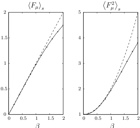
hFµis
[image:31.595.210.439.112.321.2] F2 µ ® s β β
Figure 2.2: Comparison of simulation results, numerical integration (solid line) and weak selection approximation (dashed line) when selecting with varying selection strength. Simulations are for a population of 100 whose fitnesses are drawn from a unit Gaussian and are averaged over 10 000 selections.
Using the Gram-Charlier expansion, these integrals may be calculated analytically for a truncated set of cumulants. The result is a series expansion in β
hFµis = K1+K2β+. . .
Fµ2®
s = K2+K 2
1 + (2K1K2+K3)β+. . .
Fµ3®
s = K3+ 3K1K2+K 3 1 +
¡
3K1K3+ 3K22+ 3K12K2+K4
¢
β+. . .
Fµ4®
s = K4+ 3K 2
2 +K14+ 6K12K2+ 4K3K1
+¡
4K2K13+ 4K1K4+ 12K22K1+ 10K3K2+ 6K3K12
¢
β+. . . .
(2.25)
2.3. STEADY STATE SELECTION 19
2.3.4 Small Beta Expansion
Using the terms derived above and an equivalent set forhFn
νis, found by substituting
−β for β, the cumulants after selection when using Boltzmann deletion may be found
hK1is = K1+
2K2
P β+. . .
hK2is = K2−
2K2
P2 +
2K3
P β +. . .
hK3is = K3−
6K3
P2 +
2K4
P β+. . .
hK4is = K4−
14K4
P2 −
12K2 2
P2 +. . . . (2.26)
The case of random deletion can be calculated simply by using
Fµn®
s =hF n
i (2.27)
where h. . .i represents the average over the population. The resulting expressions are
hK1is = K1+
K2
P β+. . .
hK2is = K2−
2K2
P2 +
K3
P β+. . .
hK3is = K3−
6K3
P2 +
K4
P β+. . .
hK4is = K4−
14K4
P2 −
12K2 2
P2 +. . . . (2.28)
The two sets of expressions are clearly very similar. The most obvious difference is simply the factor of two in each term containing the selection strength β. The strategy of deleting members using the Boltzmann weighting leads to a doubling of the effective selection strength. In the weak selection limit, doubling the selection strength and deleting at random is equivalent to using Boltzmann deletion.
2.3.5 Comparison with Simulation Data
2.4. COMPARISON OF GENERATIONAL AND STEADY STATE GA 20
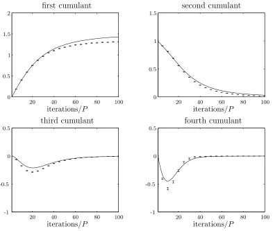
first cumulant second cumulant
third cumulant fourth cumulant
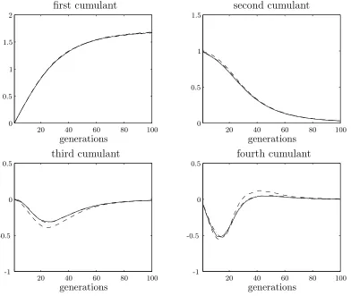
[image:33.595.133.526.117.450.2]iterations/P iterations/P iterations/P iterations/P 20 20 20 20 40 40 40 40 60 60 60 60 80 80 80 80 100 100 100 100 0 0 0 0 0.5 0.5 0.5 0.5 1 1 1.5 1.5 2 -0.5 -0.5 -1 -1
Figure 2.3: Theory predictions plotted against experimental data averaged over 10 000 runs for a simple steady state genetic algorithm using weak selection. The population size is 100 and the selection strength,β, is 0.05.
The theoretical results are calculated using the weak selection expansions for the first six cumulants. The agreement between theory and simulation is qualitatively good. For better quantitative agreement, more cumulants may be calculated.
2.4 Comparison of Generational and Steady State GA
The weak selection expansions for all three selection schemes — Boltzmann deletion, random deletion and generational — allow an easy comparison. The two steady state expressions have terms to 1/P2 rather than 1/P as they describe the change
2.4. COMPARISON OF GENERATIONAL AND STEADY STATE GA 21 The terms independent of selection strength,β, describe the change in the popula-tion due to the stochastic nature of the selecpopula-tion scheme — genetic drift. Both the steady state selection schemes exhibit double the rate of genetic drift seen in the generational case. This doubling is due to the extra randomness introduced in the choice of which population member is deleted.
When β = 0, selection is independent of fitness and the new population is simply randomly sampled from the original. In this case the expressions decouple and become exact
hK2is =
µ 1− 1
P
K2 generational selection
hK2is =
µ 1− 2
P2
K2 steady state selection. (2.29)
In an empirical comparison of generational and steady state GA, De Jong [6] noted an increase in a measure he called allele loss. This relates approximately to the increased rate of genetic drift inherent in steady state cases. Interestingly, in popu-lation genetics this comparison was performed in the nineteen fifties by Moran [21]. Although the analysis was quite different, the same doubling in genetic drift was observed as discussed in chapter eight.
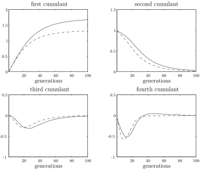
Figure 2.4 shows a comparison of simulation results for generational selection and steady state selection with random deletion. Both use a population size of 100 and a selection strength of 0.05. The increased rate of genetic drift in the steady state genetic algorithm causes the variance to decrease more rapidly. Ultimately this results in a final lower mean fitness.
Interestingly, the three cases can be shown to give approximately the same dynamics by rescaling the parameters. Since Boltzmann deletion exhibits twice the selection strength and twice the rate of genetic drift it gives rise to the same dynamics but in half the time — P/2 selections being equivalent to one generation. The same is the case for the steady state genetic algorithm with random deletion if the selection strength is doubled. Figure 2.5 shows the strong selection results overlaid with this rescaling of parameters. The time scales of the steady state algorithms plotted at
2.5. DISCUSSION 22
first cumulant second cumulant
third cumulant fourth cumulant
[image:35.595.133.526.117.450.2]generations generations generations generations 20 20 20 20 40 40 40 40 60 60 60 60 80 80 80 80 100 100 100 100 0 0 0 0 0.5 0.5 0.5 0.5 1 1 1.5 1.5 2 -0.5 -0.5 -1 -1
Figure 2.4: Comparison of generational (solid line) and steady state (dashed line) selec-tion using random deleselec-tion. Populaselec-tion size is 100 and selecselec-tion strength,β, is 0.05.
2.5 Discussion
The formalism developed by Pr¨ugel-Bennett and Shapiro gives a theoretical ground-ing on which to base investigations. The analysis of steady state selection shows that by careful theoretical comparison, results can be elucidated which have defied empirical comparisons. The results of this analysis however were dependent on the weak selection approximation and the derivation of the truncated expressions.
Whilst under the formalism as presented, the use of Boltzmann selection appears to ease the calculations, it also leads to a number of disadvantages. The large number of coupled equations required to describe the dynamics of the system mean that whilst quantitative analysis may be performed accurately, qualitative insights are still difficult in all but the simplest cases.
2.5. DISCUSSION 23
first cumulant second cumulant
third cumulant fourth cumulant
[image:36.595.134.526.119.450.2]generations generations generations generations 20 20 20 20 40 40 40 40 60 60 60 60 80 80 80 80 100 100 100 100 0 0 0 0 0.5 0.5 0.5 0.5 1 1 1.5 1.5 2 -0.5 -0.5 -1 -1
Figure 2.5: Comparison of steady state with random deletion (dashed line), steady state with Boltzmann deletion (dot-dashed line) and generational selection (solid line) when parameters are rescaled. Population size is 100 and for the generational genetic algorithm selection strength,β, is 0.05. Steady state genetic algorithms are rescaled asP/2 iterations equal to one generation.
from a finite one. In an infinite population, the mean of the distribution increases unceasingly. Clearly a finite population can only evolve as far as the fittest member of the initial population and thus the finite population effects must be calculated very accurately to capture this behaviour. An infinite population approximation is of no benefit.
Perhaps the strongest objection of the genetic algorithm community is that Boltz-mann selection is not commonly used in practice and the weak selection required for the expansions to hold is an unrealistic restriction.
Chapter 3
Genetic Drift in Selection Schemes
3.1 Introduction
Genetic drift is a term borrowed from population genetics where it is used to de-scribe changes in gene frequencies through neutral sampling of the population. It is a phenomenon observed in genetic algorithms due to the stochastic nature of the selection operator, and is one of the mechanisms by which an initially diverse population can converge to a population ofP identical members.
In chapter two, the formalism developed by Pr¨ugel-Bennett and Shapiro was used to analytically compare the dynamics of the generational and steady state genetic algorithm. In the weak selection limit, it was seen that the significant difference between the two is a doubling in the rate of genetic drift. Such a calculation is complex and some other technique is sought to calculate genetic drift in general selection schemes.
Analysis of genetic drift is often performed by calculating the Markov chain transi-tion matrices and hence finding the time for the system to reach an absorptransi-tion state where all population members are identical. This measure is commonly known as the convergence time. Comparisons in the genetic algorithm literature are often performed numerically in this fashion [5, 40]. In population genetics some work has been to done to solve this analytically however the results are approximations and are difficult to generalise to other cases [21, 13, 9].
Chapter two showed that the change in mean fitness at each generation is a function of the population fitness variance. At each generation this variance is reduced by two factors. One factor is selection pressure producing multiple copies of fitter
3.2. POPULATION FITNESS VARIANCE 26 population members. The other factor is independent of fitness and is due to the stochastic nature of the selection operator — genetic drift. By considering neutral selection, the effect of selection pressure is decoupled and genetic drift seen directly.
This chapter presents a method of calculating the rate of genetic drift in terms of this change in population fitness variance. Unlike calculations in terms of convergence time, this approach lends itself to an exact analytical solution. A general expression for the change in population fitness variance due to genetic drift is derived and applied to a range of selection schemes.
Generational and steady state selection is compared. Using the concept of genera-tion gap,G, introduced by De Jong [5, 6] to describe the percentage of the popula-tion selected from the initial populapopula-tion at each time step, the rate of genetic drift is calculated between the two extremes.
The formalism is also extended to other non-traditional selection schemes such as that used in Eshelman’s CHC algorithm [8]. Schaffer et al. [40] recently used a numerical Markov chain comparison to show that a simple model of CHC style selection exhibits half the rate of genetic drift of the traditional genetic algorithm. This is shown to be the case analytically.
The simple model of the CHC algorithm is equivalent to selection schemes in evo-lution strategies and the approach is generalised for these selection schemes.
3.2 Population Fitness Variance
For an initial population ofP discrete members, each with fitness F, the variance,
κ2, of the population fitness distribution is simply
κ2 = hF2i − hFi2
= 1
P
P
X
α=1
Fα2−
à 1 P P X α=1 Fα !2 . (3.1)
Separating terms that are not independent gives
κ2 =
µ 1 P − 1 P2 ¶ P X α=1
Fα2− 1 P2
X
α6=β
FαFβ. (3.2)
A selection scheme is then applied to this population and a new population of
3.2. POPULATION FITNESS VARIANCE 27 population memberαand the variance of the new population fitness distribution is
κ2 =
1
P
P
X
α=1
nαFα2−
à 1 P P X α=1
nαFα
!2
. (3.3)
Again separating terms that are not independent gives
κ2 = P X α=1 µ nα P − n2α
P2
Fα2−X
α6=β
nαnβ
P2 FαFβ. (3.4)
To consider the average case, the average over all ways of performing selection is taken. In the case of neutral selection, nα is independent of Fα and these terms
may be taken outside the summation. The expected population fitness variance is
hκ2is=
µ hni
P −
hn2i
P2
¶ P X
α=1
Fα2− h
nαnβi
P2
X
α6=β
FαFβ. (3.5)
As the selection scheme must maintain a constant population size, hni = 1. This gives the identity
à P X
α=1
nα
!2
=P2 = P X α=1 n2 α+ X
α6=β
nαnβ. (3.6)
Averaging over all possible selections gives
P2 =Phn2i+P (P −1)hnαnβi (3.7)
and thus
hnαnβi=
P − hn2i
P −1 . (3.8)
Substituting this expression into equation (3.5) gives
hκ2is =
P − hn2i
P −1 " µ 1 P − 1 P2 ¶ P X α=1
Fα2 − 1 P2
X
α6=β
FαFβ
#
3.3. RESULTS 28 The term within the square brackets is simply the fitness variance of the initial population given in equation (3.2) and thus
hκ2is=
P − hn2i
P −1 κ2. (3.10)
The change in population fitness variance for any selection scheme is simply found by calculating hn2i — the expected square of the number of times any population
member is selected. This is related to the variance in the number of times any member is selected —V[n]. AsV[n] =hn2i−hni2, equation (3.10) may be rewritten
in these terms
hκ2is =
µ
1− V[n]
P −1 
κ2. (3.11)
This expression is the basis for the impending results. It describes the change in population fitness variance due to the stochastic nature of selection — genetic drift — in terms of the variance in the number of times any individual is selected.
3.3 Results
To compare each selection scheme, it is only necessary to calculate V[n]. To al-low direct comparison between traditional generational selection, the results are normalised to one generation — steady state selection is performed P times and selection with generation gapG, 1/Gtimes. The ratio ris defined as the change in variance after one generation
r = hκ2is
κ2
. (3.12)
This gives a very simple picture of the change in genetic drift for differing selection schemes. Whilst the first expression for generational selection is exact, the other expressions are approximations that are accurate to terms in 1/P.
Generational: r= 1− 1
P
Steady State: r≈1− 2
P
Generation Gap G: r≈1−2−G
P
3.3. RESULTS 29
generations
50 100 150 200
0 0 1
0.2 0.4 0.6 0.8
SSGA
[image:42.595.196.452.127.337.2]GA CHC
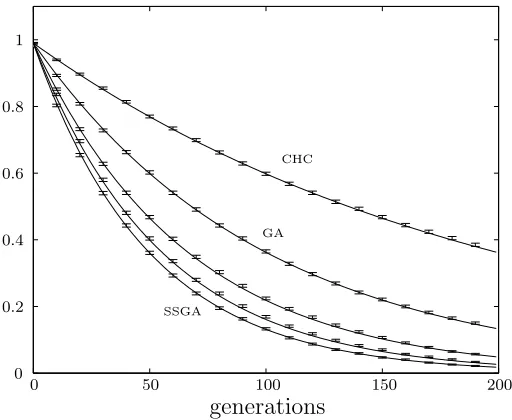
Figure 3.1: Population fitness variance for five different selection schemes. Solid lines are analytical results and error bars are simulation results averaged over 10 000 runs. Curves presented are steady state (SSGA), generation gap G=0.2, generation gap G=0.5, generational (GA), and a simple model of the CHC algorithm (CHC). Population size is 100.
The rate of genetic drift in generational selection is well known as the result of sampling P times with replacement from a finite population.
The rate of genetic drift in steady state selection is twice that of generational selection as was shown in chapter two. Varying the generation gap produces a smooth progression between these two extremes.
The simple model of the CHC algorithm shows half the genetic drift of the gener-ational selection scheme, in agreement with the empirical observations by Schaffer
et al. [40].
Figure 3.1 shows a comparison of these analytical results with simulation data. A population of 100 was initially drawn from a normal distribution (K2 = 1) and
3.4. PERFORMING THE CALCULATIONS 30
3.4 Performing the Calculations
To calculate V[n] for each selection scheme is an exercise in probability. Two results from standard probability theory regarding binomial and hypergeometric distributions are used [22].
Selecting from a population with replacement gives rise to a binomial distribution
B(N, p) where selection occurs N times with probability of successp. In this case, the variance is the number of times any individual occurs is given by
V[n] =N p(1−p).
When selecting without replacement, the result is the hypergeometric distribution
H(M, m, N). Here M is the size of the population, N is the number of times selection is applied and m is the number of copies of each individual in the initial population. This gives the result
V[n] = N m(M −N) (M −m)
M3−M2 .
In each case V[n] is calculated and used in equation (3.11) to give the expected change in population fitness variance and thus the rate of genetic drift.
3.4.1 Generational Selection
In a generational selection scheme under random sampling, P members are drawn from a population with replacement. This gives rise to a binomial distribution,
B(P,1/P) and thus
V[n] = 1−1/P.
From equation (3.11), this gives
hκ2is =
µ 1− 1
P
κ2. (3.13)
Using the definition ofr in equation (3.12) gives
r = 1− 1
3.4. PERFORMING THE CALCULATIONS 31
3.4.2 Steady State Selection
In the steady state genetic algorithm one member is selected at random, replicated and replaces another random member.
To calculate this, the population is divided into two. One member is drawn with re-placement into subpopulation A and thenP−1 members are drawn without replace-ment into subpopulation B. These two subpopulations are then combined to form the next population. Subpopulation A uses the binomial distribution B(1,1/P) and hence
V[nA] = (P −1)/P2.
Subpopulation B uses a hypergeometric distribution H(P,1, P −1) and hence
V[nB] = (P −1)/P2.
Since the two populations are independent, summing gives the final population result
V[n] = V[nA] +V[nB] = 2(P −1)/P2.
From equation (3.11), this gives
hκ2i=
µ 1− 2
P2
κ2. (3.15)
It is often more convenient to compare P of these selections to one generational selection so using the definition of r as the change after one generation
r = µ
1− 2
P2
¶P
≈ 1− 2
P. (3.16)
It is clear that the rate of genetic drift is twice that of the generational case.
3.4.3 Varying Generation Gap
3.4. PERFORMING THE CALCULATIONS 32 population.
Again two subpopulations are considered. For subpopulation A the binomial dis-tribution B(GP,1/P) is used and hence
V[nA] =G(1−1/P).
For subpopulation B the hypergeometric distributionH(P,1, P −GP) is used and hence
V[nB] =G−G2.
Summing for the final population gives
V[n] = 2G−G2−G/P.
From equation (3.11), this gives
hκ2i=
µ
1− 2G−G
2−G/P
P −1
κ2. (3.17)
To compare this to one generation, the selection operator is applied 1/G times. Thus approximating to first-order terms in 1/P gives
r = µ
1− 2G−G
2−G/P
P −1
¶G1
≈ 1− 2−G
P . (3.18)
There is a gradual transition between the two rates of genetic drift as generation gap changes.
3.4.4 CHC Algorithm
Eshelman’s CHC algorithm uses another non-traditional form of selection whereby crossover is performed amongst the initial population and then selection is per-formed without replacement from the combined population of parents and offspring.
3.5. EVOLUTIONARY STRATEGIES 33 This selection gives rise to a hypergeometric distribution H(2P,2, P) where selec-tion is performed P times from an initial population of 2P which consists of two copies of each individual.
V[n] = (P −1)/(2P −1).
From equation (3.11), this gives
hκ2i=
µ
1− 1
2P −1 
κ2. (3.19)
As we draw P members from the population, this can be compared directly to the generational case simply by making a first-order approximation
r≈1− 1
2P. (3.20)
Thus genetic drift in this model of CHC selection is at half the rate of that of the traditional generational algorithm.
3.5 Evolutionary Strategies
The model of CHC selection considered is similar to many evolutionary strategy selection schemes. The formalism presented can easily be extended to these strate-gies. In general these selection schemes are described as (µ+λ) strategies. From an initial population of size µ, λoffsprings are produced and then selection acts on both the parents and the offsprings to produce the next population of sizeµ.
Consider a (µ+λ) evolution strategy where µ = P and λ = sP where s is some fraction, 0 ≤ s ≤ 1. Selection occurs from two subpopulations, one consisting of P(1−s) individuals and the other of size 2sP containing sP pairs. If n1 is
the number of individuals and n2 the number of pairs in the final population, the
variance in the number of times any population member is selected can be shown to be simply
V[n] = 2n2
P (3.21)
asPhni=n1+ 2n2,Phn2i=n1+ 4n2 andhni= 1. The number of pairs in the final
population is simply found by considering the number of pairs produced when X
3.5. EVOLUTIONARY STRATEGIES 34
generations
s= 1
s= 1/P
s= 0.5
s= 0.2
50 100 150 200
0 0 1
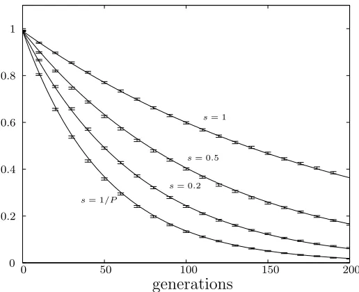
[image:47.595.195.453.125.335.2]0.2 0.4 0.6 0.8
Figure 3.2: Population fitness variance for (µ+sµ) selection for varying s. Solid lines are analytical results and error bars are simulation results averaged over 10,000 runs. Population size is 100.
size is 2sP and is given by
n2 =
X
2
X−1
2sP −1. (3.22)
Substituting equation (3.22) into equation (3.21) and averaging over X gives
V[n] = hX
2i − hXi
P (2sP −1). (3.23)
The expectations of X — hX2i and hXi — are described by a hypergeometric
distribution given by H(P(1 +s),2sP, P), as P individuals are drawn without re-placement from a population ofP(1+s). Using the standard results for the hyperge-ometric distribution given earlier and substituting these results into equation (3.23), gives the result
V[n] = 2s(P −1)
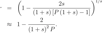
3.6. DISCUSSION 35 As before, substituting V[n] directly into equation (3.11) and normalising the ex-pression by applying selection 1/s times, gives the final rate of genetic drift
r = µ
1− 2s
(1 +s) [P(1 +s)−1] ¶1/s
≈ 1− 2
(1 +s)2P. (3.25)
The rate of genetic drift covers the same range as that seen for the genetic algo-rithm selection schemes. Figure 3.2 shows a plot of these analytical result against simulation data. Four different values of s are considered and the population size is again 100.
3.6 Discussion
[image:48.595.228.427.165.228.2]Analysing genetic drift in terms of the change in population fitness variance allows exact analytical expressions to be derived for any selection scheme. From these expressions comparisons of the effect that genetic drift has on the convergence of a genetic algorithm under varying generation gap can by made.
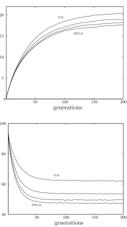
Figure 3.3 shows the population fitness mean and variance for steady state, genera-tional, and varying generation gap (G= 0.2 and 0.5) implementations of an actual genetic algorithm on the one-max problem where the fitness is proportional to the number of ones in a binary string of 96 bits. Probabilistic tournament selection is used where two individuals are drawn from the population and the fitter of the two selected with probability s. In this case s = 0.1. All use a population size of 50 and the rate of mutation at each bit is 1/96. Finally uniform crossover is perform whereby the bits of the offspring are drawn at random from two parents. CHC is not included in the comparison as the other features of the algorithm lead to more significant differences than genetic drift alone.
Selection pressure is the same in each case as evidenced by the identical initial gradients of the mean fitness curves. As variance decreases through selection, the change in mean fitness decreases. For the steady state genetic algorithm, variance decreases fastest due to the higher rate of genetic drift and thus the mean fitness evolves to a lower final value.
3.6. DISCUSSION 36
generations
50 150 200
0 5 10 15 20
100
SSGA GA
generations
50 150 200
40 60 80 100
100
SSGA
[image:49.595.198.453.178.632.2]GA
Chapter 4
Ranking Selection
4.1 Introduction
The original formalism of Pr¨ugel-Bennett and Shapiro considered Boltzmann se-lection. This has a number of features which make it attractive to the formalism, namely the easily parameterised selection strength and the exponential relationship enabling weak selection expansions to be derived.
It also has some significant disadvantages; the most commonly raised one being that it is not generally used in the genetic algorithm community. Of more significance is the weighting which is applied to the extremes of the population through the exponential relationship. These extremes are ill defined under a cumulant expan-sion and thus a large number of cumulants are required to achieve quantitatively good results. The large number of macroscopic variables required makes qualitative understanding difficult.
The extremes of the distribution are also those areas where the difference between a finite and an infinite population are most pronounced. Under a finite population, these areas are sparsely populated. This leads to finite population effects being crit-ical to the correct prediction of the dynamics of the genetic algorithm. A simplifying infinite population model is of no use as it behaves qualitatively differently.
One of the most common forms of selection in the genetic algorithm community is ranking selection or binary tournament selection. These are commonly observed to give similar results and in fact can be shown to be mathematically equivalent. For selection schemes where the weighting of each individual is a simple function of its fitness the effect of selection may be calculated exactly as previously done in
4.2. RANKING SELECTION 39 chapter two for Boltzmann selection. However in ranking selection, the additional relationship to the fitness of other members of the population makes this impossible and a new method of calculating the effect of selection is introduced.
In the analysis so far, roulette wheel selection has been considered. That is, popu-lation members are drawn with replacement from the popupopu-lation with a probability based on their weighting. This is equivalent to spinning a roulette wheel with P
unequal size bins, P times.
Whilst on average the population members are drawn with probabilities given by their weighting, the process is stochastic and there is some variance in this number. An alternative scheme suggested by Baker [2] and commonly referred to as Baker selection or stochastic universal sampling, is used to address this issue. Instead of spinning a single ball P times, a P armed pointer is spun once.
Whilst it is commonly held that Baker selection is superior, there are no theoret-ical or empirtheoret-ical comparisons beyond Baker’s original work. Under the formalism presented, the difference between these schemes can be compared.
4.2 Ranking Selection
In any selection scheme dependent on the absolute fitness value of the population members, there is a risk that an extremely fit individual will monopolise the pop-ulation. Ranking selection was suggested by Baker [1] as a means of minimising this chance and has become a standard form of selection in the genetic algorithm literature.
Rather than using the absolute values, the population is ranked in order of fitness. The expected number of times that the population member of rank i will be rep-resented in the next generation is controlled by the parameter MAX and is given by
ni = MAX−2 (MAX−1)
i−1
P −1. (4.1)
The fittest population member is expected to be represented MAX times and the least fit (2−MAX) times. MAX may take any value between one and two.
4.2. RANKING SELECTION 40
4.2.1 Infinite Population Model
In the infinite population limit, the ranking of any individual is proportional to its position within the population.
F
Thus the expected number of occurrences for an individual of fitness F is given by
nF = (2−MAX) + 2 (MAX−1)
Z F
−∞
ρ(F0) dF0 (4.2)
where ρ(F0) describes the continuous fitness distribution.
The first and second moments of the population distribution after selection are found by integrating the weighting over the distribution
hFi= Z ∞
−∞
F nFρ(F) dF
=K1 + (MAX−1)
r
K2
π
hF2i= Z ∞
−∞
F2nFρ(F) dF
=K2 +K12+ 2 (MAX−1)K1
r
K2
π . (4.3)
Thus the first two cumulants after selection are given by
hK1is =K1+ (MAX−1)
r
K2
π
hK2is =
"
1− (MAX−1)
2
π
#
K2 (4.4)
where h. . .is represents the average overall ways of performing selection.
4.2. RANKING SELECTION 41
4.2.2 Tournament Selection
Under binary tournament selection, two individuals are drawn independently from the population, compared and the fitter of the two is selected. The probability that one member of fitness F is fitter than another drawn from the population is given by
Pfitter(F) =
Z F
−∞
ρ(F0) dF0. (4.5)
When integrated over the population distribution, the result is identical to that of ranking selection when MAX = 2. Indeed the two strategies are equivalent. Changing the parameter MAX is equivalent to introducing a probabilistic element into tournament selection.
The inf