Contents lists available atScienceDirect
Computers and Mathematics with Applications
journal homepage:www.elsevier.com/locate/camwaA multi-view approach to semi-supervised document classification with
incremental Naive Bayes
Ping Gu
∗, QingSheng Zhu, Cheng Zhang
ChongQing University, Institute of Computer Science and Technology, ChongQing 400044, PR China
a r t i c l e i n f o Keywords: Co-training Multi-view Semi-supervised learning Semantic Active learning a b s t r a c t
Many semi-supervised learning algorithms only consider the distribution of word frequency, ignoring the semantic and syntactic information underlying the documents. In this paper, we present a new multi-view approach for semi-supervised document classification by incorporating both semantic and syntactic information. For this purpose, a co-training style algorithm, Co-features, is proposed. In the phase of active querying, we assign a weight to each sample document according to its uncertainty factor. Then the most informative samples are selected and labeled by other ‘‘teachers’’. In contrast to batch training mode, we developed an incremental Naive Bayes update method, which allows for more efficient training even with a large pool of unlabeled data. Experimental results show that our algorithm works successfully on the datasets Reuters-21578 and WebKB, and is superior to Co-testing in the learning efficiency.
©2008 Elsevier Ltd. All rights reserved.
1. Introduction
Text classification is the problem of automatically assigning electronic documents to pre-specified categories. Typically, text classification systems learn models of categories using a large training corpus of labeled data in order to classify new examples. Due to the tedious and subjective nature of manual labeling, labeled examples are difficult and expensive to obtain, whilst unlabeled training examples are readily available. Therefore, semi-supervised learning [1] that exploits unlabeled examples in addition to labeled ones has become a hot topic during the past few years.
A prominent achievement in this area is the co-training algorithm proposed by Blum and Mitchell [2], which trains two classifiers separately on two different views, i.e. two independent sets of features, and uses the predictions of each classifier on unlabeled examples to augment the training set of the other. For the same task, Nigam and Ghani proposed a Co-EM algorithm that uses hypotheses learned in one view to probabilistically label the examples in the other one. Intuitively, it can be seen as a probabilistic version of Co-training.
For exploiting more implicit information provided by the distribution of unlabeled examples, Muslea et al. introduce selective sampling into semi-supervised learning and propose a multi-view active learning algorithm Co-testing [3]. The main idea behind is to repeatedly train one hypothesis for each different view, then select as a query an unlabeled example where two hypotheses predict differently. To further reduce the amount of labeled data, Muslea et al. extend it again by combining Co-Testing and Co-EM and create a more robust algorithm Co-EMT [4].
The main limitation of the existing Co-training style algorithms is that they are designed to utilize only two redundant feature views, thus being unable to exploit more feature views to reduce the burden of experts and promote the final hypothesis. Moreover, in each active querying, previous algorithms require retraining with all available data. This can be a heavy burden for the user, especially when there is a large amount of training data. In this paper, we present Co-features, a new active semi-supervised learning algorithm for using a large pool of unlabeled data to improve the performance of
∗Corresponding author.
E-mail addresses:[email protected](P. Gu),[email protected](Q. Zhu),[email protected](C. Zhang). 0898-1221/$ – see front matter©2008 Elsevier Ltd. All rights reserved.
Bayes classifier. With three redundant views (lexical, semantic, syntactic information) extracted from documents, we firstly train three initial classifiers for each of redundant views. Then using uncertainty based sampling, the most informative samples are selected and asked for labeling with other classifiers. This process is repeated until none of the samples can be selected. In contrast with Co-testing and Co-EMT, in our uncertainty sampling, examples are selected and labeled without human intervention. Besides, the training process is incremental, so it does not need huge memory storage or significant computation time even with a large pool of training samples. We demonstrate the effectiveness of our proposed system via experiments with datasets Reuters-21578 and WebKB.
2. Naive Bayes classifier
Naive Bayes (NB) classifier is a simple but effective generative model, in this paper, we will choose it as the underlying supervised learner in the semi-supervised learning framework and explore an incremental Bayesian learning approach.
Letti be theith word in word dictionaryT, and
θ
=
(θ
j, θ
i|j)
be the parameters of the model, whereθ
jis the prior probability of classcj∈
C, andθ
i|jis the probability of generating wordti from the multinomial associated with classcj. Thus, the probability of generating documentxk∈
DisP
(
xk|
θ)
∝
|C|X
j=1 P(
yi|
θ)
|T|Y
i=1 P(
ti|
cj, θ).
(1)By Bayes rule, the probability that documentxk
∈
Dwas generated by classcjcan be defined as:P
(
cj|
xk, θ)
=
P(
cj|
θ)
|T|Q
i=1 P(
ti|
cj, θ)
|C|P
r=1 P(
cr, θ)
|T|Q
i=1 P(
ti|
cj, θ)
.
(2)Maximum a posteriori parameter estimation is performed by:
ˆ
θ
i|j=
1+
|D|P
k=1 N(
ti,
xk)
P(
cj|
xk)
|
T| +
|T|P
s=1 |D|P
k=1 N(
ts,
xk)
P(
cj|
xk)
(3)whereN
(
ti,
xk)
is the frequency oftioccurs inxk, andP(
cj|
xk)
is an indicator variable that is 1 whenxkhas label cjand 0 otherwise.3. Multi-views of document
BOW (Bag of Words) representation of documents has been widely used in text classification. However, one shortcoming of such methods is that they largely disregard the semantic and syntactic information underlying documents, as a consequence, are not sufficiently robust with respect to the variations in word usage. In this section, we will extend co-training by introducing two semantic and syntactic views, and use them for co-co-training of NB classifiers. Although features in three views may be slightly correlated, Nigam [5] shows that even with these, co-training is still effective in incorporating unlabeled samples.
3.1. Lexical view
Lexical view typically uses single words as features for representing document. Lettf
(
d,
t)
be the absolute frequency of wordt∈
T appears in documentd∈
D. To discount the importance of words appearing in almost all documents, we use tfidfto represent lexical feature vectors:td=
(
tfidf(
d,
t1), . . . ,
tfidf(
d,
tm))
, thetfidfof wordtin documentdis defined by:tfidf
(
d,
t)
=
log(
tf(
d,
t)
+
1)
∗
log|
D
|
df
(
t)
(4) wheredf(t)is the document frequency of wordtthat counts in how many documents.
3.2. Semantic view
Semantic view can capture the intended word sense which was ignored in literal expressions of documents. For mapping each word to its proper concept, we build on the availability of ontology like WordNet [6].
By definition, the core of ontology is a tupleO
=
(
C,
≤
c)
, which is consisted of a setC whose elements are called concept identifiers, and a partial order≤
ccalled concept hierarchy or taxonomy. Based on which, the semantical relationship between words and concepts can be revealed. Unfortunately, the assignment of words to concepts may be ambiguous in WordNet. Therefore, word sense disambiguation must be first taken to choose the ‘‘most appropriate’’ concept from thealternatives. The main steps of semantic view extraction [7,8] include:
1. Define the semantic vicinity of conceptcto be the set of all its direct sub and super conceptsV
(
c)
= {
b∈
C|
c≺
borb
≺
c}
.2. With function ref−C1
(
t)
, collect all words that express a concept from the semantic vicinity of c by U(
c)
=
S
b∈V(c)ref−C1
(
b)
.3. Collect all concepts of wordtwith refC
(
t)
, disambiguate it based on the topical context provided by documentd: dis(
d,
t)
=
first{
c∈
refC(
t)
|
cmax(
tf(
d,
U(
c)))
}
.
(5) The disambiguation strategy is very simple and intuitive: the more semantic related words appear in the same document, the more likely they share the same meaning on a given topic. For example, java is ambiguous, but its appearance in a document containing words such as island, travel, etc. is likely to isolate a given sense for that word. Thus, by referring to the term frequency of other related wordstf(
d,
U(
c))
, the most appropriate concept can be discriminated from the set of alternatives.4. Setcf
(
d,
c)
=
tf(
d,
{
t∈
T|
dis(
d,
t)
=
c}
)
and semantic feature vector to beE
td
=
(
cf(
d,
c1), . . . ,
cf(
d,
cm))
(6)wherecf
(
d,
c)
is the frequency of conceptcappears in documentdas indicated by counting all words frequency with the same meaning.3.3. Syntactic view
Each document has its own traits in the style, the syntactic information is one of the best measures to capture the stylistic divergence among different documents.
To represent the documents in vectors whose elements are syntactic information, all sentences in the documents should be chunked in the preprocessing step. In ordinary chunking, the lexical information and the POS information on the contextual words are required. Brill’s tagge [9] can be used to obtain POS tags for each word in the documents. The chunk type [10] of each word can be determined by Support Vector Machines trained with the dataset of CoNLL-2000 shared task. There are 12 types of phrases in CoNLL-2000 dataset, for example, noun phrase, verb phrase, adjective phase, O (none of these) and etc. Each phrase except O has two kinds of chunk types: B-XP and I-XP, B-XP represents the first word of the X phrase, while I-XP is given to other words in X phrase. Thus, we could find 23 types of chunk considering all combinations of IB-tags and chunk types. Simply we formulate the chunking task as a classification problem of these 23 types of chunk.
For each feature, the surrounding contexts:tj,POSj
(
j=
i−
2,
i−
1,
i,
i+
1,
i+
2),
dj(
j=
i−
2,
i−
1)
and SVMs are used to identify the chunk typediof theith wordtiin sentence. Since SVMs are basically binary classifiers and there are 23 types of chunks, SVMs are extended to multi-class classifiers by pairwise classification.4. Co-features algorithm
The question we address in Co-feature algorithm is how unlabeled data can be used to improve the accuracy of supervised learning algorithm especially in situations when: (1) only a small amount of labeled data are provided; (2) batch training of NB with the whole dataset is not feasible due to time or storage limitation; (3) no or less expert involvement is available.
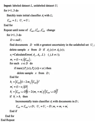
Our work mainly consists of three stages: Firstly, a new uncertainty measure based on KL divergence is presented for active selection of the unlabeled data. Secondly, a methodology for measuring the confidence in the validity of newly labeled data is introduced in order to control the classification noise during labeling. Lastly, we apply an incremental update approach to training of Bayes classifiers for improving its efficiency when faced with large training set. The pseudocode of Co-features is presented inFig. 1.
4.1. Uncertainty based selective sampling
In Co-testing and Co-EMT, uncertainty based sampling is performed by applying the classifiers to all unlabeled data and determining the contention points—the examples that are labeled differently by two classifiers. In this section, we propose a new uncertainty measure which can work only with one single Bayesian classifier.
As we have already seen, NB learning method develops the probability distribution over wordst for each given class c that accounts for the concept of that class. In this regard, we can say that if a document’s classification is uncertain under the current model, the probability distribution over the words occurring in the input document for the correct class is similar to those for other incorrect classes. From this, we find that the classification uncertainty can be determined by measuring the distances between the word distributions learned. Now, we define the new uncertainty measure based on Kullback–Leibler(KL) divergence. For documentd, the KL divergence between the word distributions induced by the classci andcjis: Uncert
(
d)
=
1−
P
ci,cj∈C KL(
P(
t|
ci),
P(
t|
cj))
|
C|
(
|
C| −
1)
(7)Fig. 1. Details of algorithm co-features.
where
|
C|
denotes the total number of pre-defined classes,P(
t|
c)
denote the distribution over wordstfor each given class, KL(
P(
t|
ci),
P(
t|
cj))
is defined as:KL
(
P(
t|
ci),
P(
t|
cj))
=
X
t∈d
P
(
t|
ci)
log(
P(
t|
ci)/
P(
t|
cj)).
(8)In most prior works, the selected samples are labeled manually. In this paper, we will avoid it by utilization of other classifier’s experience acquired in the past to label them automatically. However, none of the classifiers are 100% sure about their prediction, so additional care must be taken to control the classification noise rate when labeling of the selective samples. Assume that the selective dataset for classifierA1isD1, then for each examplex
∈
D1, we propose three criteriafor deciding whether or not to label it for next training set.
(1) Majority voting requirement, i.e., the other two classifiers must agree on the same labeling;
(2) The maximum of classifier’s confidence onxis greater than confidence threshold
α
(default is 0.7), which further ensure the reliability of prediction;However, even with this, the confidence may be overestimated, wrongly labeling is still unavoidable, our third criteria is to test if the additional data can compensate for the increase in classification noise rate. This criterion [11] is based on the following relationship between classifier’s error
, sample sizemand classification noise rateη
:m
=
1/
e2(
1−
2η)
2.
(9)To simplify our computation, we only compute the square of inverse error. More specially, in each co-training round, classifierAjandAkdecide which sample to choose for classifierAias follows:
For current classifierAi, we have the following values for sample sizem
=
L
iold
and classification noise rateη
=
mi/
L
iold. Hence our estimate for the square of inverse error isbi=
L
iold(
1−
2mi/
L
iold)
2, if examples inDwere added, the square of inverse error can be computed as:b0i
=
L
iold∪
D 1−
2(
mi+
m0i)
L
i old∪
D!
2 (10)wherem0iis the estimate of the number of examples fromDthat are mislabeled. Ifb0i
>
bi, indicating a belief thatAiwill be improved if the examples inDare added toLiold. Since our Co-features enable each classifier to label the amount of data in
each round, it tends to require fewer iterations. 4.2. Incremental Naive Bayes update
Although we cannot reduce the total number of classifications for each active sampling, we can take advantage of certain data structures in Naive Bayes to allow more efficient training of classifier and labeling of each unlabeled data. More specially, if the labeled data created during the previous co-training iterations is never revisited in subsequent iterations, the training expense can be greatly decreased.
Recall from Eq.(2)that each class probability for an unlabeled document is a product of the word probabilities for that class. When we compute the class probabilities for each unlabeled document using the new classifier, we make an approximation by only modifying some of the word probabilities in the product of Eq.(2). By propagating only changes to word probabilities for words in the putatively labeled document, we gain substantial computational savings compared to training with all documents.
Given classifierAilearned from setLiold, we can add a new documentxpwith labelcpto the training set and update the class probabilities of each unlabeled documentxiby:
P
(
cp|
xi,
θ
ˆ
0)
=
P(
cp|
xi,
θ)
ˆ
Q
t∈xi∩xp P(
t|
cp,
θ
ˆ
0)
Q
t∈xi∩xp P(
t|
cp,
θ)
ˆ
(11)whereP
(
t|
cp,
θ
ˆ
0)
is the new word probability givenLiold+
(
xp,
cp)
, andP(
t|
cp,
θ
ˆ
0)
is the old word probability given only Liold. The denominator divides out the old multinomials from the previous classifier. The product on the right-hand side
of the numerator multiplies in the new word probabilities that result from adding the newly labeled documentxp. The old multinomials that are divided out are the same as in Eq.(2). The new multinomials for the numerator can be obtained rapidly by incrementally adding to the word counts:
P
(
tk|
cp,
θ
ˆ
0)
=
1+
N(
tk,
xp)
+
LioldP
i=1 N(
tk,
xi)
P(
cp|
xi)
|
xp| + |
T| +
|T|P
k=1 L i oldP
i=1 N(
tk,
xi)
P(
cp|
xi)
(12)whereN
(
tk,
xp)
is the word frequency for wordtkin the putatively labeled documentxp. 5. Experimental evaluationTo evaluate the effectiveness of our approach, two document sets were used as test collections. The first is Reuters-21578, following other studies [12,13], we use ModApte split to form the training set and test set. From the whole dataset, we select only 10 most popular classes, which form 6649 training examples and 2545 test examples. After preprocessing, there are 7771 distinct words.
The second document set is WebKB which contains web pages from universities. This collection consists of seven categories, and each page belongs to one of the categories. In this work, only four categories course, faculty, project and student were selected. For convenience of testing, we use 20% documents as test set, the remaining 80% as training set, which result in 840 test samples and 3360 training samples.
In document preprocessing, we select top 1000 words with regard to mutual information rank. By concept mapping and text chunking, each document is also represented in the concept space(1000-dimension) and syntactic space (23-dimension) respectively.
5.1. Experimental results
In order to evaluate our uncertainty based sampling method, we first test Co-features and Co-testing on two datasets with fixed number of labeled documents 200. Except the method of sampling, other settings (three feature views, ensemble by majority voting) in the experiment are kept the same. Average accuracy and noise rate are given inTable 1for different training rounds.
As seen from above, in all cases Co-testing outperforms Co-features algorithm, it seems that our sampling method is somewhat inferior. However, if we further look into the distinction of two methods, we could find that this degrade is mainly due to the difference of two methods in labeling the unlabeled samples, Co-testing strictly relies on labeling with user, while Co-features uses only samples labeled by less accurate classifier. Considering the decrease in human effort, we think that the slight degrade of classification performance is acceptable.
Table 1
Precision and noise rate in different training round.
Dataset Round
Co-features (Precision|noise rate) Co-testing (Precision)
40 60 80 40 60 80
Reuters 79.3%|13.7% 82.0%|12.9% 83.6%|11.5% 83.7% 85.2% 86.5% WebKB 75.0%|17.3% 77.8%|15.4% 80.5%|15.5% 79.1% 81.6% 83.0%
Fig. 2. Micro-averaged F1 on the Reuters-21578 and WebKB datasets. Table 2
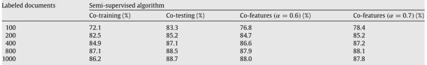
Micro-F1 on Reuters-21578 over different labeled/unlabeled training set. Labeled documents Semi-supervised algorithm
Co-training (%) Co-testing (%) Co-features(α=0.6)(%) Co-features(α=0.7)(%)
100 72.1 83.3 76.8 78.4 200 82.5 85.2 84.7 85.2 400 84.9 87.1 86.6 87.2 800 87.1 88.5 87.9 88.1 1000 86.2 88.7 88.0 87.8 Table 3
Micro-F1 on WebKB over different labeled/unlabeled training set.
Class Co-training (%) Co-testing (%) Co-features(α=0.6)(%) Co-features(α=0.7)(%)
10 20 10 20 10 20 10 20
Course 63.2 70.6 72.4 77.0 68.6 74.3 68.9 75.5
Faculty 76.0 80.3 81.5 84.4 78.2 82.5 79.7 83.9
Project 79.5 82.4 80.8 83.8 79.0 83.1 80.2 81.9
Student 70.8 73.6 75.2 80.4 74.4 77.4 75.2 79.8
Except precision, the classification noise rate for Co-features is also shown inTable 1. Note that with the progress of active learning, the noise rate decrease gradually, which further proves the effect of our error controlling in the uncertainty based sampling.
InFig. 2, we consider the effect of varying the amount of unlabeled documents. For datasets of Reuters-21578 and WebKB, we also hold the number of labeled documents and the selective samples (
|
D| =
20) constant.As shown in the figure, Co-features is capable of improving classification accuracy with unlabeled data. When labeled data is plenty and the initial parameter estimates are therefore already accurate, adding more unlabeled data tends to degrade the performance slightly. This is in accord with previous observations, e.g. (Nigram [13]). However, when only a small amount of labeled data is available, the initial parameter estimates are therefore relatively poor, unlabeled data is seen to give a significant improvement in classification performance. This algorithm is especially effective when initial few unlabeled examples are added for training, a case on which is the plots for 100 labeled documents in Reuters-21578; when unlabeled set increased by 10%, the Micro-F1 increased from 55.6% to 66.3%. Similar results can be seen in WebKB with 100 labeled documents.
We also compare Co-features with two other semi-supervised learning algorithms: Co-training and Co-testing (with two individuals).Tables 2and3contain a summary of results for different labeled/unlabeled ratio in the training set, the Column Co-features (
α
=
0.
6) shows Micaro-F1 of Co-features with threshold 0.6. For convenience of comparison, the other two algorithms are also based on NB classifiers and lexical, semantic views.Table 4
Training time (seconds) for co-features and co-testing on Reuters and WebKB.
Labeled documents Reuters-21578 WebKB
Co-testing Co-features(α=0.7) Co-testing Co-features(α=0.7)
1000 105 76 78 54
2000 264 117 184 101
3000 676 203 352 194
4000 890 415 – –
6000 1051 520 – –
Similar trend is shown inTables 2and3. In two datasets, algorithm Co-features clearly outperforms Co-training trained with labeled and unlabeled data. For example, in Reuters-21578, consider using only 100 labeled documents, our algorithm increase performance by 6.5% and 8.7% compared to Co-training. Only 200 labeled data are needed to reach the same performance with the Co-training on 400 labeled data. In WebKB, with 10% and 20% labeled data, our algorithm is uniformly better than the Co-training algorithm used in the experiment.
As a whole, Co-features is slightly inferior to Co-testing in terms of classification accuracy, especially when the number of labeled samples is small. This is caused partially by the difference of labeling method in two algorithms. In Co-testing, the samples are labeled by users, while in Co-features, the samples are labeled by less accurate classifiers. This phenomenon is also common with other incremental training algorithm, because they do not have the luxury of viewing the training set as a whole the way batch algorithms do. But in terms of running time, as shown inTable 4, our algorithm Co-features runs significantly faster than batch Co-testing algorithm.
6. Conclusions
In this paper, a new multi-view semi-supervised algorithm Co-features is presented. The main idea of which is to generate three classifiers from redundant document views: lexical information, semantic information and syntactic information. Compared with co-training, Co-features is facilitated with good efficiency and generalization ability because it could gracefully choose examples to label and update NB classifiers incrementally. Experiments on Reuters-21578 and WebKB show that using semantic and syntactic information can improve the classification performance and the unlabeled documents are good resources to overcome the limited number of labeled documents.
References
[1] A. McCallum, K. Nigam, Employing EM in pool-based active learning for text classification, Proc. Intl. Conf. Mach. Learn. (1998) 359–367.
[2] A. Blum, T. Mitchell, Combining labeled and unlabeled data with co-training, in: Proceedings of the 11th Annual Conference on Computational Learning Theory, COLT-98, 1998.
[3] I. Muslea, S. Minton, C. Knoblock, Selective sampling with redundant views, in: Proc. of AAAI-2000, 2000, pp. 621–626.
[4] I. Muslea, S. Minton, C. Knoblock, Selective sampling+semi−supervised learning=robust multi−view learning, in: IJCAI-01 Workshop on Text Learning Beyond Supervision, 2001.
[5] K. Nigam, R. Ghani, Analyzing the effectiveness and applicability of co-training, in: Ninth International Conference on Information and Knowledge Management, 2000, pp. 86–93.
[6] S. Bloehdorn, A. Hotho, Text classification by boosting weak learners based on terms and concepts, in: Proceedings of the Fourth IEEE International Conference on Data Mining, 2004, pp. 331–334.
[7] M.de Buenaga, J.M.G. Hidalgo, Using WordNet to Complement Training Information in Text Categorization, in: Recent Advances in Natural Language Processing II, vol. 189, John Benjamins, 2000.
[8] E. Agirre, G. Rigau, Word sense disambiguation using conceptual density, in: Proc. of COLING96, 1996. [9] E. Brill, A simple rule-based part-of-speech tagger, in: Proceedings of ANLP-92, 1992, pp. 152–155.
[10] Terry Copeck, Ken Barker, Sylvain Delisle, Stan Szpakowicz, Automating the measurement of linguistic features to help classify texts as technical, in: Proceedings of TALN 2000. Lausanne. 2000, pp. 101–110.
[11] S. Goldman, Y. Zhou, Enhancing supervised learning with unlabeled data, in: Proceedings of the 17th International Conference on Machine Learning, San Francisco, CA. 2000, pp. 327–334.
[12] T. Joachims, Transductive inference for text classification using support vector machines, in: Proceedings of the Sixteenth International Conf. on Machine Learning. 1999, pp. 200–209.
[13] K. Nigram, A.K. Mccallum, S. Thrun, Text classification from labeled and unlabeled documents using EM, in: Machine Learning, vol 39, 2000, pp. 103–134.