Wayne State University Dissertations
1-1-2016
Novel Machine Learning Methods For Modeling
Time-To-Event Data
Bhanukiran Vinzamuri
Wayne State University,
Follow this and additional works at:https://digitalcommons.wayne.edu/oa_dissertations
Part of theComputer Sciences Commons, and theLibrary and Information Science Commons
This Open Access Dissertation is brought to you for free and open access by DigitalCommons@WayneState. It has been accepted for inclusion in Wayne State University Dissertations by an authorized administrator of DigitalCommons@WayneState.
Recommended Citation
Vinzamuri, Bhanukiran, "Novel Machine Learning Methods For Modeling Time-To-Event Data" (2016).Wayne State University Dissertations. 1600.
by
BHANUKIRAN VINZAMURI
DISSERTATION
Submitted to the Graduate School
of Wayne State University,
Detroit, Michigan
in partial fulfillment of the requirements
for the degree of
DOCTOR OF PHILOSOPHY
2016
MAJOR: COMPUTER SCIENCE
Approved By:
This dissertation is dedicated to parents and my Guru.
I would like to extend my gratitude to my advisor Dr. Chandan K. Reddy for mentoring me throughout my PhD. I have learned a lot from his perseverance and his desire to excel in this extremely competitive world. I would also like to thank him for improving my technical writing skills and being approachable to discuss issues.
I am grateful to Dr. Ming Dong, Dr. Dongxiao Zhu and Dr. Kazuhiko Shinki for agreeing to be on my committee and I thank them for providing their valuable feedback on my research.
I would also like to thank all the PhD and Masters students of the Data Mining and Knowledge Discovery (DMKD) lab who have helped in building a productive and friendly work environment. Finally, I am indebted to my parents, sister and guru for providing necessary emotional and financial support to ensure the completion of my PhD.
DEDICATION . . . ii
ACKNOWLEDGEMENTS . . . iii
LIST OF TABLES . . . vii
LIST OF FIGURES . . . ix CHAPTER 1: INTRODUCTION . . . 1 1.1 Time-to-event Data . . . 1 1.1.1 An Illustrative Example . . . 1 1.1.2 Statistical Interpretation . . . 3 1.1.3 Main Challenges . . . 6 1.2 Our Contributions . . . 7 1.3 Organization . . . 8
CHAPTER 2: PREDICTIVE MODELS FOR TIME-TO-EVENT DATA . 10 2.1 Non-Parametric Methods . . . 11
2.2 Semi-Parametric and Parametric Methods . . . 13
2.2.1 The Proportional Hazards (PH) Model . . . 14
2.2.2 Parametric Methods . . . 17
2.3 Machine Learning Methods . . . 18
2.4 Limitations of Existing Methods . . . 19
CHAPTER 3: REGULARIZED SURVIVAL REGRESSION MODELS . . . 21
3.1 Motivation . . . 21
3.2 Preliminaries . . . 25
3.3 Cox Regression with Correlation-based Regularization . . . 27
3.3.1 FEAR-COX Algorithm . . . 28
3.3.2 OSCAR-COX Algorithm . . . 29
3.4 Experimental Results . . . 35
3.4.1 Experimental Setup . . . 35
3.4.3 Redundancy in Features . . . 39
3.4.4 Visualizing Sparsity of Models . . . 41
3.4.5 Scalability Experiments . . . 43
3.4.6 Biomarker Validation . . . 43
3.4.7 Discussion on Clinical Implications . . . 45
CHAPTER 4: REPRESENTATION BASED SURVIVAL REGRESSION . 47 4.1 Motivation . . . 47
4.2 Preliminaries . . . 50
4.3 Calibration using the Inverse Covariance Matrix . . . 52
4.3.1 REC Algorithm . . . 53 4.3.2 TREC Algorithm . . . 55 4.3.3 Algorithm Analysis . . . 57 4.4 Experimental Results . . . 60 4.4.1 Datasets Description . . . 61 4.4.2 Performance Evaluation . . . 63
4.4.3 Integrating REC and TRECwith Survival Regression . . . 64
4.4.4 Improvement in AUC with Imputed Censoring . . . 65
4.4.5 Parameter Sensitivity Analysis . . . 67
CHAPTER 5: STRUCTURED MODEL FOR RIGHT CENSORED DATA 70 5.1 Motivation . . . 70
5.2 Preliminaries . . . 72
5.3 The Proposed SLIREC Algorithm . . . 74
5.3.1 Event Matrix Generation . . . 74
5.3.2 Structured Regularization based Linear Regression . . . 76
5.3.3 Optimization . . . 79
5.3.4 Theoretical Analysis . . . 82
5.4.1 Implementation Details . . . 84
5.4.2 Evaluating Importance of Structured Regularization . . . 85
5.4.3 Evaluation using Survival Models . . . 86
5.4.4 Goodness of Survival Prediction . . . 88
5.4.5 Scalability Experiments . . . 88
CHAPTER 6: ACTIVE LEARNING BASED SURVIVAL REGRESSION . 92 6.1 Motivation . . . 92
6.2 Preliminaries . . . 96
6.3 Active Learning with Regularized Survival Analysis . . . 98
6.3.1 RegCox: Regularized Cox Regression . . . 98
6.3.2 Model Discriminative Gradient-Based Sampling . . . 101
6.3.3 Proposed ARC Algorithm . . . 102
6.3.4 Flow Diagram of ARC . . . 103
6.4 Experimental Results . . . 104
6.4.1 Datasets Description . . . 104
6.4.2 Implementation Details . . . 106
6.4.3 Goodness of Prediction . . . 107
6.4.4 Comparison of Sampling Strategies . . . 109
6.4.5 Importance of Censored Samples . . . 109
CHAPTER 7: CONCLUSIONS AND FUTURE WORK . . . 112
APPENDIX : LIST OF PUBLICATIONS . . . 115
REFERENCES . . . 124
ABSTRACT . . . 125
AUTOBIOGRAPHICAL STATEMENT . . . 127
Table 2.1 Commonly used parametric distributions in survival analysis. . . 17
Table 3.1 Notations used in this chapter. . . 24
Table 3.2 An example to demonstrate right censoring for 30-day readmission . . . 24
Table 3.3 Description of EHRs used in our experiments. . . 38
Table 3.4 Redundancy of features selected by FEAR-COX and OSCAR-COX against feature selection algorithms. . . 40
Table 3.5 Survival AUC values of FEAR-COX and OSCAR-COX against state-of-the-art algorithms. . . 41
Table 3.6 Brier score values of FEAR-COX and OSCAR-COX against state-of-the-art algorithms. . . 41
Table 3.7 Statistical association between biomarkers and heart failure readmission. 45 Table 4.1 Notations used in this chapter. . . 51
Table 4.2 Kickstarter data statistics for 18,143 projects. . . 61
Table 4.3 Description of censored statistics in the Kickstarter projects. . . 61
Table 4.4 Basic Statistics for EHRs. . . 62
Table 4.5 Comparison of Survival AUC values for different regularized Cox regres-sion algorithms without and with TREC applied on kickstarter, EHR and synthetic censored datasets. . . 64
Table 4.6 Comparison of Survival AUC values for different survival algorithms without and with TREC applied on kickstarter, EHR and synthetic censored datasets. . . 65
Table 5.1 Notations used in this chapter. . . 72
Table 5.2 Description of the datasets used. . . 84
Table 5.3 Survival AUC and standard deviation values for the SLIREC algorithm compared to other survival regression models. . . 89
Table 5.4 Integrated Brier score values for the SLIREC algorithm compared to other survival regression models. . . 89
Table 6.1 Notations used in this chapter. . . 97
Table 6.2 Description of the datasets. . . 104
Table 6.3 Comparison of Survival AUC (std) values in ARC w.r.t. different regu-larizers. . . 107
Figure 1.1 A sample illustration of survival data. . . 2 Figure 2.1 Categorization of machine learning methods for time-to-event data. . . 10 Figure 2.2 Kaplan Meier curve for data in Figure 1.1. . . 12 Figure 3.1 Correlation Heat maps for visualizing the diverse correlation structure
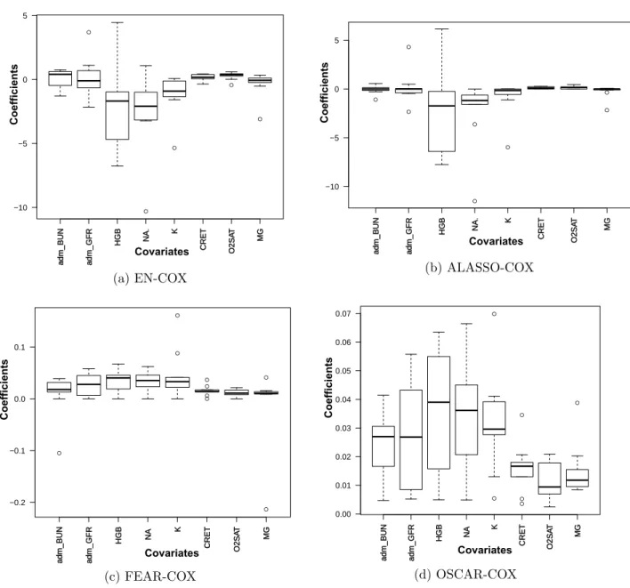
present in EHRs . . . 22 Figure 3.2 Patient readmission cycle at a hospital. . . 36 Figure 3.3 Boxplot visualizing the regression coefficients of the sparse variables
se-lected by the regularized Cox regression algorithms. . . 42 Figure 3.4 Scalability w.r.t the number of instances. . . 44 Figure 3.5 Scalability w.r.t the number of features. . . 44 Figure 4.1 Flow diagram for the proposed calibrated survival analysis approach on
a EHR dataset. . . 49 Figure 4.2 Percentage of right censored instances in EHR and Kickstarter datasets. 61 Figure 4.3 Survival AUC plots obtained for calibrated synthetic and EHR datasets
using REC, TREC, SoftImpute and Misglasso methods. . . 66 Figure 4.4 Survival AUC plots obtained for calibrated kickstarter datasets using
REC, TREC, SoftImpute and Misglasso methods. . . 67 Figure 4.5 Runtime on Kickstarter dataset usingL1, L2 norms in TREC. . . 68
Figure 4.6 Iterations for convergence usingL2 norm based TREC. . . 68
Figure 5.1 Illustrative example of SLIREC algorithm on a sample right censored dataset. . . 73 Figure 5.2 Visualizing structure in the event matrices for two survival datasets. . . 76 Figure 5.3 Performance comparison using CCA, OPLS, SSL and SLIREC methods
on various survival datasets. . . 87 Figure 5.4 Measuring improvement in runtime before and after applying the
approx-imation scheme in SLIREC for Lung dataset. . . 90 Figure 5.5 Measuring improvement in runtime before and after applying the
approx-imation scheme in SLIREC for DLBCL dataset. . . 91 Figure 6.1 Survival Regression viewed as a binary classification problem. . . 93 Figure 6.2 Active learning cycle for time-to-event data. . . 94 Figure 6.3 Block diagram of the active learning framework with KEN-COX regression.103
Figure 6.5 Comparison of the active learning rates of ARC with 4 different regular-izers over real-world and synthetic datasets. . . 110 Figure 6.6 Censoredness plot for Breast and Colon datasets. . . 111
CHAPTER 1: INTRODUCTION
Knowledge extraction from time-to-event data [1–4] is an upcoming field of research which has wide utility in different real-world applications such as healthcare, finance and engineering. Time-to-event data is different from other forms of relational data, as this data has a unique temporal structure. In such data, a domain expert monitors the occurrence of a defined event of interest. In addition, the duration of study is also defined here within which the expert monitors the event occurrence.
1.1
Time-to-event Data
In many studies, the outcome of interest is related to the timing of the occurrence of an event. This can be explained by considering a clinical setting, where one may be interested in measuring how long a chronically ill patient survives after receiving a certain treatment. In another scenario, one may be interested in determining which of the three drugs, compared to a placebo, provides symptom relief most rapidly.
Imagine that a hospital is interested in monitoring the survival status of a patient fol-lowing a first heart attack. The study could begin when the first patient, folfol-lowing his or her first heart attack, is randomly assigned to a follow-up program, with additional patients enrolled through time. Conversely, the study could begin with a cohort of subjects, each of whom has had their first heart attack, and were randomly assigned to a follow-up program. In either case, there are potentially three outcomes that could occur with each patient, with the event of interest being the death of the patient. These are (1) the patient dies; (2) the patient drops out of the study thereby becoming a loss to follow-up which could occur for any number of reasons, such as relocating geographically; or (3) the event of interest does not occur to the patient during the period of study. These three mutually exclusive events are the foundation for survival analysis studies.
1.1.1
An Illustrative Example
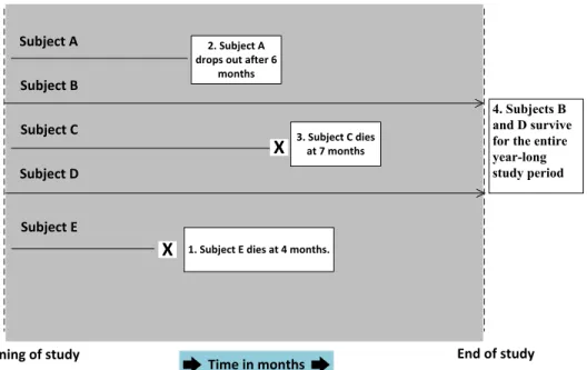
We present an illustration of time-to-event survival data which demonstrates the three cases mentioned above. In Figure 1.1, we present a simple example where 5 patients are
studied and the event of interest is the death of the patient. Subject C and Subject E have the event of interest recorded for both of them, whereas Subject B and Subject D survive the entire observation period. Their survival time is known to be for a length of time that is greater than the length of the study. This is known as type I censoring. Subject A drops out of the study after 6 months.
Survival Data
Subject A Subject B Subject C Subject D Subject E X 1. Subject E dies at 4 months. Beginning of study End of study Time in months 2. Subject A drops out after 6 months X 3. Subject C diesat 7 months 4.Subjects B and D survive for the entire year-long study period
Figure 1.1: A sample illustration of survival data.
Such instances for which the exact endpoints are not known, because the subject dropped out of the study, was withdrawn from the study, or survived beyond the termination of the study are calledright censored data, because the survival times extend beyond the right tail of the distribution of survival times. Generally, for purposes of analysis, a dichotomous, or indicator, variable is used to distinguish survival times of those subjects who experience the event of interest and those that do not because of one of the censoring mechanisms described above. Typically, this variable is called a status variable, with a zero indicating that an event did not occur and hence the survival time is censored, and a 1 indicating that the event of interest did occur.
in nature, it should be noted that there are many non-clinical uses for survival analysis as well. With the advent of computer-based statistical programs to help with complex calculations, the use of survival analysis methodologies has increased demonstrably among many disciplines. For example, engineers may wish to know the time it takes for a battery to lose its charge, a quality-control scientist at a manufacturing plant may wish to understand at which point machines need to be recalibrated, or an ecologist may want to estimate how long the average carcass remains in a study area before it is scavenged.
1.1.2
Statistical Interpretation
We now present the mathematical concepts for interpreting time-to-event data, and we also emphasize on data distributions commonly encountered in such analyses. Time-to-event data are distributed temporally, such that Time-to-events occur either at some point, or within some interval of time. These events are considered to represent a random variable having some probability of occurrence at each time period for each subject in the study. To set up the framework for survival data with right censoring, two random variables need to be defined namely, Tsurv and Tcens. The former corresponding to the survival time and the latter corresponding to the censoring time. A common censoring scheme applied to survival data is administrative censoring, where the censoring time is determined by the termination of the study. The crucial condition for the kind of survival analysis discussed here is that the survival time Tsurv and the censoring time Tcens are independent. For both the random variables the cumulative distribution functions Fsurv(t)=P(Tsurv ≤ t) and
Fcens=P(Tcens ≤t). The survival function S(t) and the censoring function G(t) are defined as given in Eq. (1.1). The observed survival time is labeled as the minimum of Tsurv and
Tcens. The censoring indicator δ is set to 0 if T=Tcens and 1 if T=Tsurv. A related concept is the cumulative hazard function denoted by H(t). H(t) and S(t) are closely related as in
H(t)=-ln(S(t)) and S(t)=exp(−H(t))
The cumulative distribution function (cdf) represents the probability that an event time is less than or equal to some specified measurement time t. F(t) is an increasing function
that runs from a value of zero (it is assumed theoretically that no events have occurred at the initiation of the study), to a value of 1 (it is assumed theoretically that all events have occurred at the conclusion of the study). In the context of survival analysis, a closely related function that is more commonly used than F(t) is a function that runs from a value of 1 (it is assumed that all subjects at the initiation of the study have survived to that point) to a value of zero (it is assumed theoretically that none of the subjects have survived when the study ends, though some subjects may be censored). Conveniently, this is known as the survival distribution, S(t), and is mathematically related to the cumulative distribution function as mentioned in Eq. (1.1).
F(t) =P(T ≤t) (1.1)
S(t) = 1−Fsurv(t) = P(Tsurv > t)
G(t) = 1−Fcens(t) = P(Tcens> t)
The probability distribution function is represented by the set of probabilities that spec-ify the possible values of a random variable. In the context of survival analysis, this density function represents the probability of an event occurring in a defined interval of time. Al-though, fully appreciating the intricacies of this probability distribution requires knowledge of calculus, we can illustrate its meaning conceptually by using some of the properties of the normal distribution. When we calculate the probabilities for the normal distribution, we are interested in calculating the area under a curve that was bounded by two values. Similarly, in survival analysis we are interested in calculating the probability of an event bounded by an interval of time, say ∆t and then finding our probability as the interval becomes very small, that is as ∆t → 0. Hence, the probability distribution function, f(t), is defined by Eq. (1.2).
f(t) = ∆F(t) ∆t =−
∆S(t)
∆t (1.2)
time defines the probability function. It is also possible to find this function by examining what happens during a change inF(t), say ∆F(t), or a change inS(t), say ∆S(t), in a given interval of time.
The mean survival time is another important metric of interest in survival analysis, which is defined as µ= E[X] and which maybe further expressed as µ=R0∞S(t)dt. This gives the expected lifetime for an individual with a given survival function which is sometimes needed in survival analysis to estimate the life expectancy. Although the hazard function is difficult to estimate directly in survival analysis, it plays an important role in understanding the process of survival. A decreasing hazard function implies that the prognosis gets better as you live longer, and an increasing hazard function implies that the prognosis gets worse as you live longer.
Finally, a function that is often encountered in survival analysis is the hazard function,
h(t). This function is used to define the instantaneous probability of an event occurring, given that the subject has survived up to a given time t. This function is defined as in Eq. (1.3).
h(t) = P(t ≤T < t+ ∆t|T ≥t)
∆t ∆t→0 (1.3)
h(t) = f(t)
S(t)
This function is based on a conditional probability, wherein we are interested in calcu-lating the probability of an event occurring given that the subject has already survived until a particular time point. The condition of having already survived to a given time means that the probability of surviving into the future is influenced by having already survived previous time periods. This idea can be very important in some situations, where surviving the early stages of a disease may dramatically decrease the potential of an event occurring in the near future. As an example, consider cancer where non-recurrence, or remission, for a period of 5 years generally increases survivorship. This function can also be expressed in terms of the two functions previously defined in Eq. (1.3). This expression is defined so
because, the hazard function can exceed 1, so it is not truly a probability, though it is based on the conditional probability of an event occurring. The hazard function is often defined in survival analysis by a known distribution such as the lognormal, exponential, or a Weibull distribution.
1.1.3
Main Challenges
We now explore the challenges that will be addressed in this dissertation while building models for time-to-event data which are as follows.
• Correlation: In longitudinal data, it is observed that the data exhibits different kinds
of correlations which are as follows (i)Inter-event correlation: Instances for which the events are observed tend to be correlated with each other. For example, two patients who were readmitted within 30-days of discharge for a disease, most often have a lot of similarity in the actions which triggered their readmission. (ii)Intra-event correlation: The covariates of an electronic health record (EHR) for a patient have a non-uniform effect in determining the survival status, which is why this intra-event correlation is an extremely important factor in predicting event occurrence.
• Missing information: During the period of observation, the events are not observed
for all the patients, because of several reasons such as loss of follow-up or early ter-mination of the study. In such cases, these patients do not have any time-to-event labels associated with them and they are called as right censored instances, as they only have a censoring time associated with them. This causes a significant problem while learning models from time-to-event data.
• Lack of adaptability: Prominent machine learning methods such as linear regression
offer several benefits when applied for prediction on right censored data. However, ex-isting linear regression-based methods are non-intuitive and they rely on user specified parameters to interpret the censoredness from the data. In such scenarios, it is ex-tremely desirable to extend the linear regression model to right censored data, so that it can interpret the inherent patterns (such as the underlying structure of the data)
and use this knowledge extensively for prediction. The motivation for this approach is that it does not rely on user specified parameters and it can make the linear regression model more adaptable to different distributions of events and censored instances in the data.
• Insufficient training instances: Models built on such data rely heavily on the
quality of training data available. Instances for which the event is observed have an event label defined and they can be added to the model directly. However, including censored instances in the model which do not have labels, has to be decided judiciously by assessing the influence of adding the instance in the model. This is a non-trivial task and the model has to include only those censored instances in the training data, which are having a significant impact on the model performance.
1.2
Our Contributions
We now mention the major contributions of the proposed machine learning models for time-to-event data. They are as follows.
• We address the problem of building survival models which can infer intra-event
cor-relation by proposing two diverse regularizers. We address two forms of intra-event
correlation which are feature based correlation and grouped correlation, respectively.
Correlation among features in survival data is addressed using the FEAture Regular-ized Cox (FEAR-COX) algorithm. Grouped correlation (structured sparsity) among covariates in survival data is addressed using the Octagonal Shrinkage Clustering Al-gorithm Regression (OSCAR-COX). The performance of these alAl-gorithms is studied exhaustively on longitudinal EHRs obtained from a large hospital. These regularizers are also compared to state-of-the-art regularization methods in the literature.
• We propose a representation learning method for imputing times for the censored in-stances, which estimates the censored times by inferring the correlation pattern among different censored instances. This method uses a novel two-dimensional imputation approach which incorporates the inter-event and intra-event correlation to estimate
the time-to-event label for censored instances using a sparse inverse covariance based imputation method. This is called the Transposable REgularized covariance based calibration method (TREC). This learned new representation of the original survival dataset using TREC is then used for subsequent survival analysis.
• We present a method called Structured regularization based LInear REgression al-gorithm for right Censored data (SLIREC) which infers the underlying structure of the survival data directly and uses this knowledge to guide the base linear regression model. This structured approach is more robust compared to the standard statistical and Cox-based methods, as it can automatically adapt to different distributions of events and censored instances in the dataset which is very useful when dealing with different real-world datasets.
• We propose an active learning based survival regression method which can efficiently identify important censored instances from the survival dataset which are contribut-ing most in order to build an effective survival model. This active learncontribut-ing method is generic as it uses the gradient of the loss function employed in the learning algo-rithm. We implement this active learning approach using the regularized Cox regression framework to present the Active Regularized Cox (ARC) algorithm.
1.3
Organization
This dissertation is organized as follows. In Chapter 2, we present an overview of popular survival analysis methods such as non-parametric, semi-parametric and ensemble methods, and conduct an in-depth literature study on different models for time-to-event data in these three categories. In Chapter 3, we present our regularized Cox regression algorithms which proposes two correlation-based regularizers to handle diverse intra-event correlation in longi-tudinal data. In Chapter 4, we present our representation learning based survival regression algorithm which is successful in learning a novel representation for survival data. This algo-rithm infers the time-to-event label using an imputation-based inverse covariance method. In Chapter 5, we present our Structured regularization based LInear REgression algorithm
for right Censored data (SLIREC) which extends the linear regression model by making it more adaptable to right censored data. In Chapter 6, we present our active learning-based survival regression approach, which is the first method to successfuly use the active learning methodology for survival data to obtain a model with more informative and lesser number of training instances. Finally, in Chapter 7, we draw conclusions from all these algorithms and briefly discuss methods for extending them.
CHAPTER 2: PREDICTIVE MODELS FOR TIME-TO-EVENT DATA
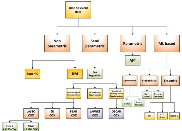
In this section, we present the related work on existing machine learning methods pro-posed for time-to-event data. We provide a flow diagram in Figure 2.1 which represents different kinds of methods described in this chapter.Time‐to‐event data
Non
parametric Parametric ML based
Semi parametric
SuperPC KM RegressionCox
AFT
Optimization Probabilistic Ensemble
Feature based Regularization Graph based Regularization Structured Sparsity based Regularization LASSO COX EN COX FEAR COX LAPNET COX OSCAR COX Fused LASSO COX ADAP LASSO COX SVM NetworkNeural Naïve Bayes Bayesian Network
RSF BoostCOX Boost CI
Figure 2.1: Categorization of machine learning methods for time-to-event data.
In this chapter, we discuss about different non-parametric estimation methods [4, 5]. This is followed by explaining the most important semi-parametric method studied in the survival analysis literature called Cox regression [6]. We study its partial log-likelihood formulation in detail. We segregate the existing methods for time-to-event data into three categories, namely, non-parametric, semi-parametric and parametric methods. Non-parametric methods such as the Kaplan-Meier (KM) and Nelson-Aalen (NA) estimator directly conduct inference
on the data without making any assumptions about the distribution. Semi-parametric meth-ods make a trade-off between non-parametric and parametric methmeth-ods by trying to extract information from the covariates present in the dataset, and they do not make any additional assumptions on the distribution of the hazard function [1–3].
Parametric methods, on the other hand, make assumptions apriori on the distribution of the functions involved completely and conduct maximum likelihood estimation for learning the model parameters directly. These methods make assumptions which seem to be confined to a fixed distribution alone while conducting survival analysis which need not be the case with survival data sampled from multiple distributions. This is the main motivation to prefer semi-parametric methods over parametric methods in survival analysis. We now study each of these methods in detail in the following sections.
2.1
Non-Parametric Methods
Non-parametric methods are used frequently for survival analysis as they make no as-sumptions about the hazard function and conduct estimation. We start by explaining the Kaplan-Meier (KM) estimator. The starting point for the KM estimator is considering a sample of n independent observations (t1, δ1),(t2, δ2), . . . ,(tn, δn) from (T,δ). The following notation is introduced from the field of counting processes.
ˆ SKM(t) = Y s≤t 1− 4¯N¯(s) Y(s) (2.1)
Let Yi(t)=1{ti ≥t}, ¯Y(t)=Σni=1Yi(t),Ni(t)=1{ti ≤t,δi = 1}, ¯N(t)=Σni=1Ni(t). The risk set R(t) = {i;ti ≥ t} represents the set of instances who are at risk at a given time t, and
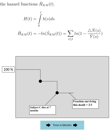
4N¯(t) is the number of events at time t. This KM estimator is one of the most widely used non-parametric estimators of the survival function. It can be interpreted as a conditional survival function resulting from a partitioning of the time scale and estimating the survival function on each partitioning. In Figure 2.2, we plot the KM curve for the data considered in Figure 1.1. This KM estimator can also be defined similarly for the censoring function
ˆ
GKM(t) and the hazard functions ˆHKM(t).
H(t) = t Z 0 h(s)ds (2.2) ˆ HKM(t) = −ln( ˆSKM(t)) = X s≤t ln(1− 4¯N¯(s) Y(s) )
Corresponding Kaplan-Meier Curve
100 % Subject C dies at 7 months Fraction surviving this death = 2/3 Time in Months
Figure 2.2: Kaplan Meier curve for data in Figure 1.1.
We now look at other methods for non-parametric survival analysis such as supervised principal components (SuperPC). This is a method which selects features from survival data which have a direct effect on the time-to-event. The steps involved in this algorithm involve computing the standard regression coefcients for each feature and then form a reduced data matrix consisting of only those features whose univariate coefcient exceeds a pre-defined threshold in absolute value. Subsequently, the selected principal components of the reduced data matrix are used in a regression model to predict the time-to-event outcome [7].
Multiple imputation for censored data is a method where the failure times are imputed using an asymptotic data augmentation scheme based on the current estimates and the baseline survival curve [8]. Once this is done a standard procedure such as Cox regression is
applied to the imputed data to update the estimates. A similar problem has been dealt with in the crowdsourcing domain which predicts the time-to-event directly using the survival function [9, 10]. Misglasso is an extension to the approach for imputing missing values by using the graphical lasso algorithm [11–13]. Other popular approaches include the SoftIm-pute algorithm which uses a nuclear norm minimization subject to constraints to fill the missing entries [14].
Risk stratified imputation in survival analysis is another approach which performs strat-ified imputation of missing time-to-events based on groups of patients who are similar to each other. The stratification is done to ensure that not too many samples are imputed, and all the imputation is done among censored instances which are similar to each other. An auxiliary variable approach to multiple imputation in survival analysis is proposed here [15] with the goal to improve efficiency using Monte Carlo methods.
2.2
Semi-Parametric and Parametric Methods
Cox regression is a semi-parametric method which uses the proportionality hazards (PH) assumption. It is widely used because of its effective performance and ease of availability. However, due to its maximum likelihood-based formulation, Cox regression tends to overfit data. This problem is solved by introducing regularizers into Cox regression to reduce the variance of the obtained solution.
The Lasso regularizer which is based on the L1 norm was integrated with the partial
log-likelihood function and the corresponding optimization problem was solved using the iteratively reweighted least squares algorithm. Lasso provides sparse solutions, but when selection has to be conducted over several correlated variables it selects one variable and does not consider the remaining variables. The elastic net regularizer which uses a convex combination of theL1andL2norms is effective for correlated survival data and the elastic net
Cox (EN-COX) algorithm is implemented using a cyclic coordinate descent algorithm [16]. The computation in this algorithm is accelerated by approximating the Hessian computation involved. To incorporate more feature-based information, graph regularization has also been
used with Cox regression, where the graph Laplacian is used as a penalty [17–19]. The graph laplacian can successfully capture feature similarities through its structure and this penalty tries to keep similar coefficient values for connected features in the graph. Such graph-based regularized Cox models can also be stabilized using the regularizers built on the feature graph. The Jaccard graph is used here to obtain stability in the model. In a similar way, the adaptive lasso regularizer can also be used with Cox regression which improves performance over the LASSO-COX model [20–22]. In this algorithm, LASSO-COX is applied on the survival dataset, then the inverse of the obtained regression coefficients are used as weights to run further rounds of the LASSO-COX algorithm. This approach was observed to be more biased towards features initialized with higher weights, but it obtained superior performance in many cases. Fused-lasso is a similar regularizer which imposes sparsity on the model by imposing temporal smoothness among the regularizer coefficients to ensure stability of the coefficient values. Regularizers such as scout were also integrated with Cox regression [23]. These come under the supervised covariance-based regression models which consider the covariance matrix over the features and impose sparsity on it. The inverse covariance matrix represents the partial correlations between different features present in the dataset and this method can be considered as a minor variant of the feature correlation-based regularizers described above.
2.2.1
The Proportional Hazards (PH) Model
A very popular model in survival analysis is the proportional hazards (PH) model where individual specific hazard functionshi(t) are learned, and the proportional hazards assump-tion is made as given in Eq. (2.5). In this model,ci is constant andh0(t) is a baseline hazard
function which is left unspecified. The ci term can be replaced withexp(XTβ) to obtain the Cox PH model [24].
hi(t) =cih0(t) (2.3)
The effect of the covariates on the hazard can be modeled by taking ci=exp(XiTβ). The survival function implied by the model is given in Eq. (2.4) where H0(t)=
Rt
0 h0(s)ds is the
cumulative baseline hazard and the baseline survival function is given asS0(t)=exp(−H0(t)).
S(t|X) = exp(−exp(XTβ)H0(t)) =S0(t)exp(X
Tβ)
(2.4)
A key feature of Cox regression model is that the hazard function of two individuals with covariates X0 and X00 respectively are proportional. This can be expressed as in Eq. (2.5) and this ratio is constant over time. This ratio is called the relative risk for an individual with covariates X0 compared toX00
h(t|X0) h(t|X00 ) = h0(t)exp(X 0 β) h0(t)exp(X 00 β) =exp[β T(X0−X00)] (2.5)
The Cox regression model learns the regression coefficient vectors in survival analysis using a method called the partial likelihood estimation. We now explain this concept by first looking at the complete log-likelihood using the information summarized in the dataset in the form of triplets (T, δ, X) as in Eq. (2.6)
L(h0, β) =
n
X
i=1
(−H0(ti)exp(xTi β) +δi(ln(h0(ti)) +xTi β) (2.6)
Expanding this equation usingH0(t) =
P
s≤th0(s) gives us Eq. (2.7) and for a fixed value
of β this expression is maximal for the breslow estimator, which is given as in Eq. (2.8).
L(H0, β) = X t (−h0(t) X i Yi(t)exp(xTi β) +ln(h0(t))4N¯(t) + X i 4Ni(t)xTi β)) (2.7)
Substituting the Breslow estimator in Eq. (2.7) gives us Eq. (2.9). In this equation,pl(β)
represents the partial log-likelihood which is given in Eq. (2.10). ˆ h0(t|β) = 4N¯(t) P iYi(t)exp(xTjβ) (2.8)
A simplified and more often used version of the partial likelihood is provided in Eq. (2.11). L( ˆh0(β), β) =pl(β) + X t − 4N¯(t) +ln(4N¯(t)) (2.9) pl(β) = n X i=1 ∞ Z 0 ln( exp(x T i β) P jYj(t)exp(x T jβ) )dNi(t) (2.10) pl(β) = k Y i=1 exp(βTXi) P j∈Riexp(β TX j) (2.11)
Finally, we also present the logarithmic version of this partial likelihood which is often used for MLE estimation in Cox regression in Eq. (2.12).
l(β) = log(pl(β)) = k X i=1 βTXi− k X i=1 log(X j∈Ri exp(βTXj)) (2.12)
The computation of the partial log-likelihood is changed if we consider tied event times in survival data. For all thek unique time-to-event values we usedi to represent the number of times ti re-occurs in the survival data andDi to represent the set of indices with time ti. In addition, we also let si = Pj∈DiXj then the approximations proposed by Breslow and Effron can be found in Eq. (2.13).
l(β)breslow = k Y i=1 exp(βTsi) P j∈Riexp(β TX j)di (2.13) l(β)ef f ron= k Y i=1 exp(βTsi) Qdi j=1[ P h∈Riexp(β TX h)− jd−1i P l∈Diexp(β TX l)]
The computation in Cox regression consists of maximizing the partial log-likelihood given in Eq. (2.12) with or without the ties adjustment as given in Eq. (2.13), and then using the estimated regression coefficient vector in the estimating functions given in Eq. (2.14) to obtain the time dependent survival function. There are two ways to estimate the survival function one is using the NA estimator and the other is using the analogue of the KM
estimator which is called the Product-Limit (PL) estimator. These are provided in Eq. (2.14). ˆ SN A(t|X,βˆ) = exp −Hˆ0(t)exp(xTβˆ) (2.14) ˆ SP L(t|X,βˆ) = Y s≤t 1−exp(xTβˆ)ˆh0(s)
2.2.2
Parametric Methods
Parametric methods differ from semi-parametric methods, as these assume that the haz-ard distribution is specified. The accelerated failure time (AFT) model is one of the popular parametric survival models. We look at its formulation briefly. The AFT model assumption is stated in Eq. (2.15) whereS0 is the baseline survival function. From this equation it is seen
that covariates act multiplicatively on time so that their effect is to accelerate or decelerate time-to-event relative to the basline survival function.
S(t|X) =S0(t)exp(X
Tβ)
(2.15)
An equivalent popular formulation of AFT-model is the following linear regression for-mulation for the log-transformed event timelog(T) given X as in Eq. (2.16).
log(T) =−XTβ+. (2.16)
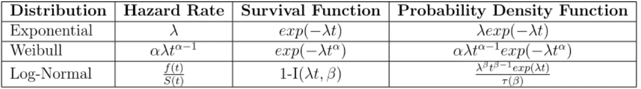
In this equation is assumed to be independent of X. The AFT model is appealing due to its direct relationship between the failure time and the covariates. The semi-parametric version of the AFT model is computationally intensive, but if we are willing to specify a form for the baseline function, then the AFT model is fully parametric. We also specify some of the commonly used parametric distribution in survival analysis in Table 2.1.
Table 2.1: Commonly used parametric distributions in survival analysis.
Distribution Hazard Rate Survival Function Probability Density Function
Exponential λ exp(−λt) λexp(−λt)
Weibull αλtα−1 exp(−λtα) αλtα−1exp(−λtα)
Elastic net Buckley James (EN-BJ) [25] is a method which directly models the response for events using the least squares method, and for the censored instances the response variable is imputed using the conditional expectation values given the corresponding censoring times and covariates. This algorithm uses the elastic-net regularization term with this AFT model and was applied on high-dimensional genomic data obtaining good performance.
2.3
Machine Learning Methods
In this section, we present the machine learning methods used for analyzing time-to-event data. We categorize these methods into three categories, namely, (i) Bayesian-based (ii) Optimization-based and (iii) Ensemble-based. Censored Naive Bayes (CensNB) is a bayesian approach which applies the standard Naive Bayes algorithm for censored data [26]. In this algorithm, the conditional survivor function is learned by initializing the functions using non-parametric densities, which are then subsequently smoothed using a weighted loess smoother. These models use an approach called inverse probability of censoring weighting (IPCW) for each of the records in the dataset. This is a method which applies weights to the censored instances inorder to account for censoring when compared to uncensored instances (events). Similarly, bayesian networks based data imputation has also been used to enhance the performance of survival trees. The imputation on missing instances is done using the bayesian network computed on complete instances and the model has shown to perform well in clinical trials.
We now look at ensemble methods for time-to-event data. The first method in this category is CoxBoost which applies the boosting based paradigm to the Cox regression al-gorithm by building a set of weak learners and learning their weights iteratively. A more refined boosting framework for survival data is based on boosting the concordance index (BoostCI) [27]. This method is based on optimizing the evaluation metric such as concor-dance index (survival AUC) directly, rather than optimizing the maximum likelihood, which has been observed to perform better in several scenarios. The algorithm computes the neg-ative gradient of the concordance index and fits it separately to each of the components of
X and continues this until convergence is observed.
Random Survival Forests (RSF) is an ensemble method which uses a forest of survival trees for prediction [28]. The basic intuition of the RSF algorithm is explained as follows. The algorithm begins by drawingB bootstrap samples from the original data where 37% of the data is excluded in each sample which is also called out-of-bag (OOB) data. A survival tree is grown for each sample, where at each node we randomly selectp candidate variables. The node is split using the candidate variables that maximizes survival difference between the daughter nodes. A constraint is used so that no terminal node has less than d0 unique
deaths. An ensemble cumulative hazard function is calculated using the cumulative hazard function for each tree and the OOB data is used to evaluate the model. This approach was found to provide competitive performance for many survival datasets.
Apart from this method other extensions to the linear regression model have been studied extensively in the context of multi-response prediction. These include methods such as canonical correlation analysis (CCA) [29], orthonormalized partial least-squares (OPLS) [30] and shared subspace learning (SSL) [31] which attempt to reduce the dimensionality of high-dimensional data and try to learn a projected representation onto the lower high-dimensional space. Subsequently, regression models built on the learned projected space perform more effectively.
2.4
Limitations of Existing Methods
We now look at the limitations of the methods discussed above. Non-parametric methods such as KM, NA, CensNB and SuperPC are flexible to use, but they do not conduct any form of inference on the survival data. Real-world survival data often needs some additional interpretation through the form of methodical inference of its properties, so that effective models can be built on them. In this dissertation, in Chapter 4, we study two different representation learning-based algorithms which modify the representation of survival data by capturing inherent properties such asintra-event andinter-event correlations in the dataset. This helps in deciphering patterns in the survival data which can enhance the predictive
power of the base model.
Semi-parametric regression methods such as Cox regression suffer from the overfitting problem, due to its MLE formulation. Traditional real-world survival data has complex patterns which cannot be deciphered using simple regularizers such as the lasso and ridge. In Chapter 3, we study more advanced properties in survival data such as structured sparsity in the form of grouped correlation to propose regularizers to handle such data.
Survival data consists of both events and censored instances, and the model is built using information from both these sources. However, the reliability of the information obtained from censored instances is ambiguous, as they do not have defined time-to-event labels. The models mentioned above directly use the censored times for these instances during model building, which is inappropriate. In this problem, it is extremely important to determine the influence of a censored instance on the model before including it in the training model. The survival models mentioned above do not address this labelling problem with survival data which is crucial to build reliable and effective models. These issues are addressed in detail in Chapter 6.
CHAPTER 3: REGULARIZED SURVIVAL REGRESSION MODELS
3.1
Motivation
The necessity to build correlation-based regularized Cox regression algorithms can be explained by considering the heterogeneous nature of electronic health records (EHRs) [32– 35]. A typical EHR can be obtained by concatenating data from several resources such as demographics, comorbidities, procedures, medications, labs and insurance information. We segregate all this information from a real EHR cohort considered in this dissertation, and we plot the canonical correlation heatmaps between each of these groups. Canonical correlation captures the correlation patterns among multi-dimensional datasets with the same number of instances and different number of features by calculating the weights of the projection vectors which maximize the correlation between these two datasets in the projected space. This makes canonical correlation heat maps ideal to visualize the diverse correlation structure in EHRs.
The correlation heat maps in Figure 3.1 indicate that the intensity of correlation among the 6 different subgroups of EHRs are high, and this correlation pattern should be effec-tively utilized by an algorithm to obtain accurate predictions. One can also observe that as the correlation patterns are not uniform, which indicates the necessity to build complex regularizers that can account for such heterogeneous and non-uniform grouped correlation structure in EHRs.
In this chapter, we propose two algorithms which integrate novel regularizers in the Cox regression framework, which addresses two forms of intra-event correlation, which are feature correlation and grouped correlation, respectively. We present a generalized framework which converts Cox regression to a modified least squares problem using the gradient and Hessian information from the partial log-likelihood of Cox regression. This framework can be inte-grated with any regularizer using the corresponding regularized least squares version solver. For example, the traditional shooting LASSO least squares solver [36] can be integrated
di-−1.0 −0.5 0.0 0.5 1.0 value demographics l abs (a) Demographics-Labs −1.0 −0.5 0.0 0.5 1.0 value demographics medications (b) Demographics-Medications −1.0 −0.5 0.0 0.5 1.0 value demographics procedures (c) Demographics-Procedures −1.0 −0.5 0.0 0.5 1.0 value demographics insurance (d) Demographics-Insurance −1.0 −0.5 0.0 0.5 1.0 value comorbidities demographics (e) Comorbidities-Demographics −0.5 0.0 0.5 1.0 value comorbidities l abs (f) Comorbidities-Labs
Figure 3.1: Correlation Heat maps for visualizing the diverse correlation structure present in EHRs
rectly with this framework to provide a more effective solution for LASSO-COX. We use this framework exhaustively, and study a total of 7 regularized Cox regression methods of which we implement 4 methods, namely, (fused-lasso (FLASSO-COX), adaptive-lasso (ALASSO-COX), feature regularized (FEAR-COX) and oscar (OSCAR-COX) using this least squares framework.
We propose a Feature Regularized Cox regression (FEAR-COX) algorithm which uses a novel feature-based regularizer with the modified least squares formulation of Cox regres-sion. Our experimental results demonstrate that this method is more effective than the elastic net at handling correlated features. The novel pairwise feature similarity regularizer in this method is obtained using a convex formulation which uses a positive semi-definite matrix. We propose a graph-based OSCAR (Octagonal Shrinkage and Clustering Algorithm for Regression) regularized Cox regression method (OSCAR-COX) which uses the oscar reg-ularizer [37] based least squares solver with the modified least squares formulation of Cox regression. This method is effective since it can capture structured sparsity (grouped corre-lation) among the feature sets in EHRs. It exploits the graph structure of the features in the dataset to capture this unique phenomenon in EHRs.
We demonstrate the improved discriminative ability of FEAR-COX and OSCAR-COX using standard evaluation metrics in survival analysis such as concordance index (c-index) and brier score. We also demonstrate the non-redundancy of the features selected by the sparse models of FEAR-COX and OSCAR-COX and also visualize the sparsity of our pro-posed models. In addition, we use the parsimonious models from FEAR-COX and OSCAR-COX to identify important biomarkers for heart failure readmission from EHRs. We validate the biomarkers identified using well known survey studies from the clinical informatics liter-ature.
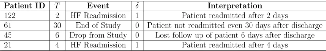
We now present a synthetic example which illustrates how patients are right censored in an EHR setting. In Table 3.2, we consider a simple EHR dataset consisting of 4 instances. In this example, the time is measured in days. The censoring time is set to 30 days for all
Table 3.1: Notations used in this chapter.
Name Description
X n x m matrix of feature vectors
T k x 1 vector of sorted unique failure times
Ri risk set of all patients j such that (tj ≥ti)
di number of patients readmitted within time ti
δ n x 1 vector of censored statu.
ˆ
β m x 1 regression coefficient vector
S(·),G(·), h(·) survival, censoring and hazard functions
Fsurv(·), Gcens(·) cumulative survival and censoring functions
P Positive semi-definite feature regularizer matrix
E incidence graph on feature set
the patients. One can observe that instances with patient ID 122 and 21 are not censored and hence δ is set to 1 with the survival time equivalent to the time to event of interest (T). Instances with patient ID 61 and 45 are censored withδ set to 0. In this manner, right censoring is applied on the instances in the dataset.
Table 3.2: An example to demonstrate right censoring for 30-day readmission
Patient ID T Event δ Interpretation
122 2 HF Readmission 1 Patient readmitted after 2 days
61 30 End of Study 0 Patient not readmitted even 30 days after discharge
45 6 Drop from Study 0 Lost follow up of patient 6 days after discharge
21 4 HF Readmission 1 Patient readmitted after 4 days
With a brief description of the survival regression framework, we now introduce some notations that will help in comprehending the Cox regression framework in Table 3.3. Given a dataset X which consists of n data points. Let xi denote the ith feature vector. Let
T = {t1 < t2 < t3 < . . . < tk} represent the set of sorted k unique time-to-event values.
δi represents the censoring status for the ith patient. δi=1 represents the occurrence of an event andδi=0 represents a censored instance.
3.2
Preliminaries
The likelihood term in Cox regression can be written as in Eq. (3.1) and the partial log likelihood is defined using Eq. (3.2).
l(β) = n Y i=1 ( exp(xTi β) P j∈Riexp(x T jβ) )δi (3.1) L(β) = log(l(β)) = n X i=1 δixTi β− n X i=1 δilog X j∈Ri exp(xTjβ) (3.2)
In the partial log likelihood equation, Ri is the set of all patients who are in the risk set of the ith patient. In this Equation, the covariate values for the jth individual is represented using xj. ∂L(β) ∂βj = n X i=1 δixij − n X i=1 δi P l∈Riexp(x T l β)xlj P l∈Riexp(x T l β) (3.3) ∂2L(β) ∂βj∂βk =− n X i=1 δi " P l∈Riexp(x T l β)xljxlk P l∈Riexp(x T l β) (3.4) − P l∈Ri(exp(x T l β)xlj)Pl∈Ri(exp(x T l β)xlk) P l∈Ri(exp(x T l β))2 #
We now explain the procedure to convert Cox regression to a modified least squares problem. We define these additional notations to explain our interpretation of Cox as a modified least squares problem. In Algorithm 3.1, M is a triangular matrix obtained after applying the Cholesky factorization on H.M is called the pseudo-design matrix. zis denoted as the pseudo-response vector.
In Algorithm 3.1, the calculation of a pseudo-design matrix (M) and a pseudo-response matrix(z) helps us solve Cox regression problem as a modified least squares problem. This is very helpful considering that there are state-of-the-art least squares solvers which can then be used for solving different variants of Cox regression problems. Similarly, penalized Cox regression problems can also be converted into penalized least squares problems which then
become easier to solve with the existing solvers. However, the Hessian calculation in Cox regression is computationally expensive which can hinder the performance of Algorithm 3.1. It is so because for each of the m2 elements of the matrix we have to compute the risk
sets individually. So we use a trick here to improve the performance of the algorithm by accelerating the Hessian computation. We set theH matrix to be equivalent to the diagonal matrix of the elements of the diagonal of -∂β∂2L(β)
j∂βk.
Finally in Algorithm 3.1, we estimate the values of ˆβ iteratively until convergence is obtained. Once the regression coefficient vector ˆβ is estimated, we can obtain the baseline hazard function using Eq. (3.5). After obtaining the baseline hazard function, we can com-pute the hazard function h(t) for any given time t. This gives us the hazard or survival probability estimates at any given timet with the trained Cox model.
h0(t) = X i:ti≤t δi P j∈Riexp( ˆβ Tx j) (3.5)
Algorithm 3.1: Cox regression as a modified least squares problem
1 Input: Time-to-event labels T, Censored survival dataX, Censoring Indicatorδ,
Number of instances n, tolerance parameter tol, Maximum iterations
itermax.
2 Output: Regression coefficient vector ˆβ
3 Initializeβ;
4 Derive the partial log-likelihood function L(β) using Eq. (3.2);
5 for j=1 to itermax do 6 Set G=−∂L∂β(β) j using Eq. (3.3); 7 Set H =−∂ 2L(β) ∂βj∂βk using Eq. (3.4); 8 Compute M ←cholesky(H); 9 Compute z←(MT)−1·(Hβ−G)); 10 Solve arg min
β (z−M β)T(z−M β); 11 if kβ−βˆk2< tol then 12 break; 13 end 14 Set β = ˆβ; 15 end
3.3
Cox Regression with Correlation-based Regularization
In this section, we describe the algorithms developed by combining two novel correlation-based regularizers with Cox regression. We integrate both these regularizers following the same paradigm explained in Algorithm 3.1 where we convert Cox regression into its equivalent least squares formulation (LSQ). This conversion helps us solve a regularized Cox regression problem as a regularized least squares problem itself. This is a very critical part of all the regularized Cox regression methods we discuss in this chapter including those presented in Section 3.4. We do not explicitly mention this conversion in the discussion below and only discuss the solutions for the regularized least squares variants itself to great detail. Finally, we use these derived regularized least squares solvers in Step 9 of Algorithm 3.1 to obtain the desired regularized Cox regression algorithm.
We now briefly discuss about how the regularizers presented in this section differ from the most commonly used regularizers. Generally, most regularizers considered in the literature are convex loss functions because of their desirable properties. The motivation for applying convex functions in the clinical domain arises from the success achieved by using convex non-smooth functions such as the L1 and the L2,1 norms for different applications [38].
Their properties of sparsity and group sparsity have proven to be very effective for such applications.
Our novel regularizers are functions which use the L1, L2, and L∞ norms. Regularizers
also need a parameter which governs their importance in the framework. In general, this is denoted as λ and is also called the regularization parameter. In this section, we present the regularizers and their corresponding optimization routines used in the different variants of the modified least squares formulation of Cox regression. This is followed by exploring the feature based penalty and the Octagonal Shrinkage and Clustering Algorithm for Regression (OSCAR) penalty. We now explain how these penalties can be integrated in the modified least squares formulation of Cox regression, and then we present efficient solvers which are later integrated in Algorithm 3.1 to obtain the FEAR-COX and OSCAR-COX algorithms,
respectively.
3.3.1
FEAR-COX Algorithm
In this section, we define the feature-based regularizer for the modified least squares formulation of Cox regression, and we then discuss the cyclic coordinate descent method for solving this optimization problem. This regularizer is defined in the context of the least squares problem as follows. Consider a linear model as given in Eq. (3.6) whereX ∈Rn×m is the data matrix, y∈ Rn is the response vector andβ is the regression coefficient vector. We can assume that the model is standardized which implies that 1Ty=0, 1TX
i=0 andXiTXi=1
y =Xβ+. (3.6)
The general problem being solved is given in Eq. (3.7). In this equation J(β) is a non-negative valued penalty function. λ is a non-negative complexity and regularization parameter. For the least squares formulationJ(β)=0. For ridge regression J(β)=kβ k2
2 and
for the lasso J(β)=kβ k1. The overall minimization formulation will be as follows
ˆ
β= arg min β
ky−Xβ k2 +λJ(β) (3.7)
We propose a feature-based convex regularizer and plug it into the regression framework. The regularizer is used to incorporate the pairwise feature similarity into the regression framework. Let P ∈ Rm×m be a positive semi-definite matrix.
J(β) = |β|TP|β| (3.8)
ˆ
β = arg min β
ky−Xβ k2 +λ|β|TP|β|
feature-based regularizer in Eq. (3.8). L(β) =ky−Xβ k2 +λ|β|TP|β| (3.9) =yTy−2qTβ+βTQβ+λX i,j Pij|βiβj| ∂L ∂βi =−2qi+ 2QTi β+ 2λsgn(βi) m X j=1 Pij|βiβj| (Qii+Pii)βi+sgn(βi)λ X j6=i Pij|βj|=qi− X j6=i Qijβj
In Eq. (3.9), we provide the cyclic coordinate descent steps used in solving for β. We set
Q=XTX and q=XTy. This is followed by setting the derivative to zero and solving for the
ith coordinate of β keeping the remaining (i-1) components constant. In this formulation, S is the soft-thresholding function and is defined as Sλ(x)=sgn(x)max(|x| −λ,0).
To implement the FEAR-COX algorithm, we follow the steps outlined in Algorithm 3.1 and replacing the Equation in Step 9 of Algorithm 3.1 by the FEAR-COX solver procedure provided in Algorithm 3.2. This replacement in Algorithm 3.1 makes use of a more efficient regularizer in the form of the feature-based formulation to learn the corresponding regression coefficient vector.
3.3.2
OSCAR-COX Algorithm
Structured sparsity (grouped correlation) in EHRs as illustrated in Figure 3.1 is a phe-nomenon which is difficult to capture using regular sparsity inducing norms such as the LASSO and elastic net. In practical applications, one often knows a structure on the co-efficient vector in addition to sparsity. For example, in group sparsity, one assumes that variables in the same group tend to be zero or nonzero simultaneously. If meaningful struc-tures exist, we show that one can take advantage of such strucstruc-tures to improve the standard sparse learning based Cox regression methods. In this algorithm, we incorporate the OSCAR (Octagonal Shrinkage and Clustering Algorithm for Regression) regularization [37] into the Cox regression framework.
Algorithm 3.2: Solver for the FEAR-COX Algorithm.
1 Input: Feature Vector X, Response variable y, Regularization parameter λ, PSD
MatrixP, Maximum number of iterations numiter, Tolerance tol, Initialized coefficient vector β0
2 Output: Regression vector β
3 Initializeβ0; 4 Q←XTX, q←XTy, βold ←β←β0; 5 for j=1 to numiter do 6 for i=1 to m do 7 βi ← S(Qiiβi−Q T iβ+qi,λ(PiT|β|−Pii|βi|)) Qii+λPii ; 8 end
9 if kβ−βoldk2< tol then
10 β ←diag(1 + QPii ii)β; 11 return; 12 end 13 βold ←β; 14 end
OSCAR performs variable selection for regression with many highly correlated predictors. The advantage of using this penalty over other penalties such as the elastic net and LASSO is that this method promotes equality of coefficients which are similarly related to the response. OSCAR obtains the advantages of both individual sparsity due to theL1norm and the group
sparsity because of the pairwise L∞ norm. It can select features and form different groups
of features. In this way, OSCAR also does supervised clustering of the features. In this chapter, we use the modified Graph OSCAR (GOSCAR) regularizer [37, 39, 40] in the Cox regression formulation. The formulation of the GOSCAR penalty is given in Eq. (3.10). In this formulation,E is the incidence matrix of the feature graph and L(β) is the loss function which is the modified least squares loss function derived from the partial log likelihood of Cox regression andλ1 and λ2 are the regularization parameters.
In this manner, a pairwise feature regularizer is added to the Cox regression formulation. OSCAR has proven to be more effective than the elastic net in handling correlation among variables and hence is more suited for EHR data as illustrated in Figure 3.1. For the sake of simplicity, we refer to the GOSCAR-COX algorithm as OSCAR-COX throughout this
chapter.
ˆ
β =arg min
β
L(β) +λ1(kβ k1) +λ2(kEβ k1) (3.10)
In contrast to the FEAR-COX algorithm, the formulation in OSCAR-COX is non-smooth. This problem can be solved using the alternate direction method of multipliers (ADMM) [41] method effectively. The ADMM method has proven to have a very fast con-vergence rate and is particularly useful for our problem. We now explain the OSCAR regres-sion algorithm for regularized linear regresregres-sion which can be used for solving the modified least squares formulation of OSCAR-COX. This solution will use the ADMM formulation for fast and efficient convergence. We now explain the formulation for the alternate direction method of multipliers (ADMM).
The ADMM routine is used to solve problems of the form in Eq. (3.11). The variables
x ∈ Rn and z ∈
Rm where A ∈ Rp×n, B ∈ Rp×m and c ∈ Rp. f and g are assumed to be
convex functions.
arg min
x,z f(x) +g(z) (3.11)
s.t. Ax+Bz =c
ADMM method uses a variant of the augmented lagrangian method and reformulates the problem as given in Eq. (3.12). The update rule steps which are iteratively processed in this method are given in Eq. (3.13). In Eq. (3.14), we provide a basic formulation of the OSCAR penalty in the linear regression setting explained above.
Lρ(x, z, µ) = f(x) +g(z) +µT(Ax+Bz−c) (3.12)
+ρ
2 kAx+Bz−ck
The update rule for ADMM is given by xk+1 : = arg min x Lρ(x, zk, µk) (3.13) zk+1 : = arg min z Lρ(xk+1, z, µk) µk+1 : =µk+ρ(Axk+1+Bzk+1−c)
The GOSCAR regression algorithm uses the OSCAR penalty with a least squares loss function. This is a modified form of the OSCAR penalty as given in Eq. (3.14) with the addition of the incidence matrix E for the graph. We now explain the steps needed to solve this modified OSCAR regression problem using the ADMM procedure. The ADMM formulation for the GOSCAR regression algorithm is given in Eq. (3.15).
arg min β ky−Xβ k 2 +λ1 kβ k1 +λ2 X i<j max{|βi|,|βj|} (3.14) arg min β,q,p 1 2 ky−Xβk 2 +λ 1 kq k1 +λ2 kpk1 (3.15) s.t β−q= 0, Eβ−p= 0 Lρ(β, q, p, µ, v) = 1 2 ky−Xβ k 2 (3.16) +λ1 kqk1 +λ2 kpk1 +µT(β−q) +vT(Eβ−p) + ρ 2 kβ−qk 2 +ρ 2 kEβ−pk 2 βk+1 = arg min β 1 2 ky−Xβk 2 +(µk+ETvk)Tβ (3.17) +ρ 2 kβ−q k k2 +ρ 2 kEβ−p kk2
Algorithm 3.3: OSCAR Solver for the modified least squares formulation of Cox Regression.
1 Input: Feature Vector X,Response y,Incidence Graph E, Regularization
parameters λ1, λ2, Auxiliary parameter ρ, Maximum number of iterations itermax
2 Output: Regression vector βk
3 Initializep0 ←0, q0 ←0, µ0 ←0, v ←0;
4 for k=1 to itermax do
5 Compute βk+1 using Eq. (3.17); 6 Compute qk+1 using Eq. (3.18); 7 Compute pk+1 using Eq. (3.18); 8 Compute µk+1, vk+1 using Eq. (3.18);
9 k ← k + 1;
10 Continue until convergence; 11 end qk+1 = arg min q ρ 2 kq−β k+1 k2 +λ 1 kqk1 −(µk)Tq (3.18) =Sλ1/ρ(βk+1+ 1 ρµ k) pk+1 =Sλ2/ρ(Eβk+1+ 1 ρv k) (3.19) µk+1 =µk+ρ(βk+1−qk+1) vk+1 =vk+ρ(Eβk+1−pk+1)
In this formulation, q and p are the slack variables. E is the incidence matrix of the graph. In Eq. (3.16), we obtain the augmented lagrangian function in terms of the variables and lagrange multipliers µ and v. In this equation, ρ is the scalar augmented lagrangian parameter which is derived using cross validation.
In Eq. (3.18), Sλ is the soft thresholding function. Sλ(x)=sgn(x)max(|x| −λ,0). To implement the OSCAR-COX algorithm, we follow the steps outlined in Algorithm 3.1 and replace the Equation in Step 9 of Algorithm 3.1 by the OSCAR solver for the least squares formulation of Cox provided in Algorithm 3.3.
The essence of both FEAR-COX and OSCAR-COX is the same that they are solving a regularized least squares problem derived from Cox regression. However, the difference arises in the usage of novel regularizers and different optimization methods for solving the regular-ized least squares problem. In terms of the regularization, the difference between the FEAR and OSCAR regularizers lies in their uniqueness in handling correlated variables. FEAR uses a feature-based regularizer in its formulation to handle correlated variables effectively. In this algorithm, the choice of P is important, but we do not study the performance with different formulations of P which is intended for future work. It uses the L2 norm based
formulation in its regularizer.
In OSCAR, we use the L1 norm and a pairwise L∞ norm term. The pairwise L∞
func-tion encourages similar coefficient values for correlated variables. OSCAR is also effective at handling structured sparsity which cannot be inherently detected using the elastic net reg-ularizers. This discussion helps us understand that both these algorithms handle correlated variables in their own unique ways.
We now discuss the complexity of these algorithms. FEAR-COX uses the cyclic coordi-nate descent approach with a convex smooth composite loss function which is theoretically known to converge from the literature of coordinate descent. The time complexity of one iteration of FEAR-COX is O(m) which is for the soft-thresholding operation.
OSCAR-COX uses the ADMM method coupled with a convex loss function. The theory of augmented lagrangian based multipliers can be used easily here to prove the convergence of this approach using the ADMM steps provided earlier in this section. In OSCAR-COX, the Cholesky factorization only needs to be computed once, and each iteration involves solving one linear system and two soft-thresholding operations. The time complexity of the soft-thresholding operation is O(m). Due to the sparsity of computing the incidence matrix
E, its time complexity is O(me), where e is the number of edges in the feature graph. Thus the time complexity for one iteration of OSCAR-COX is O(m(m + n) + me).
3.4
Experimental Results
In this section, we discuss the experimental results obtained by using the proposed FEAR-COX and OSCAR-FEAR-COX regression algorithms on 9 real-world EHRs. We evaluate the goodness of these algorithms in terms of non-redundancy in feature selection, discrimina-tive ability measured using the survival AUC (concordance index) and Brier score metrics, respectively. We compare the performance of our proposed regularizers against state-of-the-art regularizers such as adaptive-lasso (ALASSO) [20, 42], laplacian net (LAPNET) [43] and fused-lasso (FLASSO) [44]. We also provide brief implementation details for these algorithms and the parameter settings are also explained. Our feature selection analysis compares the goodness of the features selected using our methods and compares them to those obtained from other prominent feature selection methods for censored data. We also plot the sparse important variables included in the models and conduct a study on the biomarkers obtained by using the proposed algorithms and validate those biomarkers using survey articles from existing clinical literature.
3.4.1
Experimental Setup
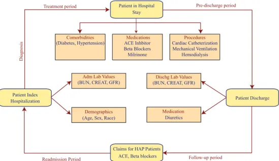
In this section, we provide the description of the components of the EHRs used in this chapter followed by briefly explaining the implementation details for our proposed regularized Cox regression algorithms. We will describe various kinds of variables present in our data acquired from Henry Ford Health System (HFHS) Detroit, Michigan USA. We also present a flowchart diagram which represents how these variables are collected from a patient at HFHS in Figure 3.2. The patient readmission cycle consists of the different stages a patient goes through from the initial admission to the next readmission [45, 46]. The different kinds of information obtained from the patient beginning from the admission to discharge includes demographics, comorbidities, medications, procedures and pharmacy claims. All these constitute an EHR for that particular hospitalization of the patient. The entire set of important variables which constitute an EHR are classified in the literatur