Parallelization of backward deleted distance calculation in graph based features using Hadoop

(1)

PARALLELIZATION OF BACKWARD DELETED DISTANCE CALCULATION IN GRAPH BASED FEATURES USING HADOOP

by

JAYACHANDRAN PILLAMARI

B.E., Osmania University, 2009

A REPORT

submitted in partial fulfillment of the requirements for the degree

MASTER OF SCIENCE

Department of Computing & Information Sciences College of Engineering

KANSAS STATE UNIVERSITY Manhattan, Kansas

2013

Approved by: Major Professor Dr. Daniel Andresen

(2)

Abstract

The current project presents an approach to parallelize the calculation of Backward Deleted Distance (BDD) in Graph Based Features (GBF) computation using Hadoop. In this project the issues concerned with the calculation of BDD are identified and parallel computing technologies like Hadoop are applied to solve them. The project introduces a new algorithm to parallelize the APSP problem in BDD calculation using Hadoop Map Reduce feature. The project is implemented in Java and Hadoop technologies.

The aim of this project is to parallelize the calculation of BDD thereby reducing GBF computation time. The process of BDD calculation is examined to identify the key places where it could be parallelized. Since the BDD calculation involves calculating the shortest paths between all pairs of given users, it can viewed as All Pairs Shortest Path (APSP) problem. The internal structure and implementation of Hadoop Map-Reduce framework is studied and applied to the process of APSP problem. The GBF features are one of the features set used in the Ontology classifiers. In the current project, GBF features are used to predict the friendship relationship between the users whose direct link is deleted. The computation involves calculating BDD between all pairs of users. The BDD for a user pair represents the shortest path between them when their direct link is deleted. In real terms, it is the shortest distance between them other than the direct path. The project uses train and test data sets consisting of positive instances and negative instances. The positive instances consist of user pairs having a friendship link between them whereas the negative instances do not have any direct link between them. Apache Hadoop is a latest emerging technology in the market introduced for scalable, distributed computing across clusters of computers. It has a Map Reduce framework used for developing applications which process large amounts of data in parallel on large clusters.

The project is developed and implemented successfully and has the best time complexity. The project is tested for its reliability and performance. Different data sets are used in this testing by considering various factors and typical graph representations. The test results were analyzed to predict the behavior of the system. The test results show that the system has best speedup and considerably decreased the processing time from 10 hours to 20 minutes which is rewarding.

(3)

iii

4.2.1. Unit Testing .……..…………..………...…… 34 4.2.2. Performance Testing .………..……….………...…… 36 4.2.2.1. Speedup ………..………... 38 4.2.3. System Testing .………...…… 38 4.3. Results ….………..………...…… 39 4.3.1. Bottlenecks …………..………... 39 Chapter 5 - Conclusion .………..………...…… 40 5.1. Limitations .……….…..………...…… 40 5.2. Future Work .………….………...…… 40 References .……...………...…… 41

(5)

v

List of Figures

Figure 2.1 Figure 2.1.3 A Sample Graph showing GBF features ………..… 6

Figure 2.4.2 Datanode and Namenode managing files in the form of blocks [9] ……… 13

Figure 2.4.3.1 Distribution of data across different nodes [9] ……….…………....… 14

Figure 2.4.3.2 Map Reduce pipeline on different nodes [9] ………....… 14

Figure 2.4.3.3 Internal Structure of Map Reduce data flow [9] ………...……....… 15

Figure 3.1 Sample 5-Node Graph .………...……… 20

Figure 3.1.1 Pseudo code - Building Adjacency Graph .………..……… 21

Figure 3.1.1.1 Sample Input Graph - Building Adjacency Graph .………..………....… 21

Figure 3.1.1.2 Output Graph of Building Adjacency Graph using Map Reduce ….………....… 22

Figure 3.1.2.1 Pseudo code for Running Parallel APSP Map Reduce .………....… 24

Figure 3.1.2.2 Iteration-0 Graph - Running Parallel APSP Map Reduce ………....… 26

Figure 3.1.2.3 Iteration-1 Graph - Running Parallel APSP Map Reduce ……… 26

Figure 3.1.2.4 Iteration-2 Graph - Running Parallel APSP Map Reduce ………....… 27

Figure 3.1.2.5 Iteration-3 Graph - Running Parallel APSP Map Reduce ………..….. 27

Figure 3.1.2.6 Iteration-4 Graph - Running Parallel APSP Map Reduce ……… 28

Figure 3.1.2.7 Iteration-5 Graph - Running Parallel APSP Map Reduce …….…..………...… 28

Figure 3.3.1 Class Diagram ……….………..…..… 31

Figure 3.3.2.1 Context Level Diagram ………..……..… 32

Figure 3.3.2.2 Level-0-DFD - Extracting network data and generating instances …..…..…..… 32

Figure 3.3.2.3 Level-0-DFD - Building Adjacency Graph ………..…..………..… 33

Figure 3.3.2.4 Level-0-DFD - Running Parallel APSP Map Reduce ………..……..…..… 33

Figure 4.2.1 Test Results for Unit Testing ………...………….……...… 36

(6)

vi

List of Tables

Table 2.3.1.1 Software Requirements - Pseudo Distributed mode ………...……... 10 Table 2.3.1.2 Software Requirements - Fully Distributed mode ………...………...…..…. 10 Table 2.3.2.1 Hardware Requirements - Pseudo Distributed mode ………...…………...…..…. 12 Table 2.3.2.2 Hardware Requirements - Fully Distributed mode ………...……. 12 Table 4.2.1 Test Cases for Unit Testing ………..………....……. 35 Table 4.2.2 Test Results of Performance Testing ……..………...…………...……. 37

(7)

vii

Acknowledgements

I would like to acknowledge this project to my major professor Dr. Daniel Andresen, without his support this project would not have been possible. I am grateful to him for his suggestions and comments. I also appreciate his help and constant guidance throughout my project. I am thankful to Dr. Doina Caragea and Dr. Mitchell Nielsen for graciously accepting to be on my committee and giving their valuable time to review my report. I am thankful to them for their guidance and suggestions.

(8)

- 1 -

Chapter 1 - Introduction

In the recent years there is a significant growth of social media and its awareness among the people. It has made a great impact on social interaction of internet users. Though the primary use of it is to make networking with online users, there have been lots of other uses associated with it. It has showed its effect on the business world also. Many companies are interested in finding out the user interests to increase their sales and improve business productivity. Different business individuals use social media to make connections and listen to the customers. This revolution lead to a research in the area of social media called social network analysis. The graph theory is used for modeling social networks. With the increase in social networking sites there grew a need for better algorithms in the area of graph theory to improve the methodologies for social network analysis. The analysis mainly involves graph search problem computations. The current project tries to deduce a solution to one of the graph search problems of social network analysis.

The importance of this project comes from the fact that the graph search problems are also used in other fields like path tracking systems. The Path Tracking and Navigation systems are used predominantly worldwide by many individuals and companies. Most of the car drivers are highly depended on the navigation systems software. The path advice demand is growing and there is need for the navigation software to be improved. While it is easy to retrieve the shortest paths using navigation software, most of the data provided by them is pre-calculated. Sometimes it is necessary to calculate the all possible shortest paths and these computations last very long. The routes and road paths will be changing from day to day and there is need for the navigation software providers to update their systems very frequently. Because these calculations take very long time, there is need for a better system to compute the shortest paths with in a real time. As the calculations are in quadratic to the number of nodes, the systems memory may not be capable holding the whole data. We need a system which can deal with the graph theory problems effectively.

1.1 Problem Description

The current project deals with friendship prediction problem in social network analysis. The following describes the problem context for the current project. Social network analysis deals

(9)

- 2 -

with different approaches in analyzing and visualizing the social networks. Some of the sub tasks include: finding user interests, determining trustworthiness of user generated content, object classification, link prediction and friendship prediction. The task of friendship prediction uses different types of features sets and Graph Based Features (GBF) are one of them. The GBF features are found to be quite effective in predicting the friendship for a given user pair in a social network. Live Journal social network data is one of the data set used for GBF computation. The specialty of Live Journal social network is that it lays emphasis on user interaction [10].

The problem faced by the current researchers in GBF computations is that it takes lot of time to compute the GBF features. A GBF computation includes the calculation of Backward Deleted Distance (BDD), which is the area where it takes a lengthy time. The BDD calculation involves finding the minimum alternative distance between all pairs of users in the reverse direction, ignoring the direct path if exists. It actual terms it is an All Pairs Shortest Path (APSP) problem. Though there are many existing solutions for the APSP problem they are not that effective and do not provide a better approach. Some of the existing solutions for All Pair Shortest Path problem are Parallel Dijkastras APSP [8], Simple Parallel Floyd Warshall APSP [7], Blocked Parallel Floyd Warshall APSP [5] and Phased Parallel Floyd Warshall APSP [6]. These current existing systems do not provide any effective solution for dealing with the APSP problem.

The existing systems are not capable of extracting true parallelism for the APSP problem. They are not capable of utilizing the resources effectively. The existing approaches have algorithms to compute for a complete network graph in distributed environment, but there are no efficient algorithms to compute for the incomplete network like disconnected graphs and directed graphs in distributed environment. Most of the algorithms are designed for a uni-processor environment. Though there are some solutions for distributed environment they are not capable of handling the parallel APSP problem effectively. Most of the existing systems computing are based on the in-memory representation of the graph. They cannot handle if the graph size or its corresponding data is large. Most of them are not scalable. They cannot provide node level granularity in their computation.

(10)

- 3 -

1.2 Motivation

A keen interest in developing a distributed application for a better cause led me to develop the current project. The project is interesting as it presents real world situations for developing highly scalable applications. It has gained an importance as the APSP graph search problem is used in many other fields. The All Pairs Shortest Path computation involves independent asynchronous calculations. The motivation for the current project comes from the idea of deducing a parallel implementation for those asynchronous calculations. A Hadoop tutorial showing parallel implementation of Breadth First Search [12] provides an insight into the current project. The tutorial gives an idea of representing graphs using colors and distances along with adjacency list which motivates us to design a better format for representing the graphs and designing a solution for the APSP problem.

1.3 Proposed System

The current project deals with examining the Graph Based Features computation and identifies the key areas where it takes a lot of time and tries to reduce them by applying parallelization, different techniques and approaches. It mainly deals with parallelization of the APSP problem in Graph based features BDD calculation. The current project introduces a new algorithm for implementing the APSP problem in parallel. It uses Hadoop, an emerging technology for scalable distributed computing with high throughput. In the current project Hadoop map reduce feature is used for parallelizing the computation. The project explores different ways for implementing node level parallelism and introduces new technique for the APSP computation. It investigates different ways of computing for directed and disconnected graphs in distributed environment. In one line to say the project presents a highly scalable and parallel computing approach for the APSP problem. It solves the Graph Based Features computation by solving for APSP problem. It also tries to reduce the time in building the graph from the given social network data.

The System is implemented mainly in two modules: Building Adjacency Graph and Running Parallel APSP Map Reduce Algorithm. They are as follows:

 Building Adjacency Graph – In this module, the given friendship links of the social network are transformed into an Adjacency List with Trio Sets Format (ALTS) using Hadoop Map Reduce.

(11)

- 4 -

 Running Parallel APSP Map Reduce Algorithm – In this module, Parallel APSP algorithm is run on the ALTS node format list graph to compute All Pairs shortest Paths for all the nodes.

The Characteristics of the current project are as follows:  Highly scalable

 provides node level parallelism  Redundancy and Failure Recovery  Less usage of Heap memory  Low Bandwidth

 High Throughput  High Speedup

 Optimal Time complexity  Cost effective

 Flexible and Fault tolerant

The rest of the paper first discusses related work with background and system analysis in Section 2. In Section 3, a detailed implementation and architecture of the system is presented. Section 4 describes how the system is evaluated and presents the results. Section 5 presents our conclusions and describes future work and limitations.

(12)

- 5 -

Chapter 2 - Related Work

2.1 Background

The current section gives a brief description about the background of the system by explaining the terminology used in the project. The different terms related to this project are Social Network Analysis, Live Journal Data, Graph Based Features, Backward Deleted Distance and Parallel APSP Problem. The following discussion briefly elaborates them.

2.1.1 Social Network Analysis

The Social Network Analysis is used for unveiling the hidden links or relationships with the use of network model. It views social relationships in terms of the network theory, which consists of nodes representing users and ties representing relationships between users. These are represented using points and lines in network theory. It maps and measures the relationships and flows between people, groups and entities in a social network. It is mainly used to analyze and visualize social network. It includes different tasks like finding user interests, predicting friendship relationship, kinship, link prediction, object classification and analyzing user generated content. They use this knowledge discovered as input for modeling social network and explore further information. The analysis of the social networks is done with the use of ontologies for varied reasons. There are different types of ontologies used for analyzing social networks like domain ontologies, reasoning ontologies and inference ontologies. These ontologies use different types of features for modeling the social network ex: interest based features and graph based features. These features computation requires social network data consisting of user generated content. There are different online services available for providing the network data and Live Journal is one of them. The current project uses the live journal network data as the input Train data.

2.1.2 Live Journal Social Network

Live Journal is an online journal service with an emphasis on user interaction [10, 11]. In the Live Journal social network, users can tag other users as friends and share their interests. It can be represented using a network graph, where nodes of the graph represent the users and the edges

(13)

- 6 -

between the nodes represent the friendship links between the users. It has 10 million on-line users and provides a free service.

2.1.3 Graph Based Features

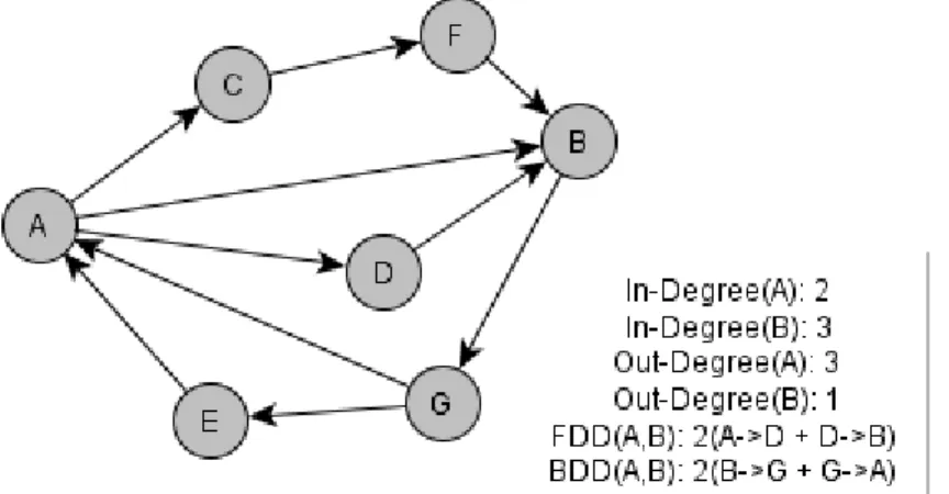
The Graph Based Features (GBF) is one of the features set used for analyzing the social networks. They are mainly used for predicting the friendship relationship and predicting the interests. The GBF features are found to be quite effective in predicting the friendship for a given user pair in a social network [11]. The Figure 2.1.3 shows the GBF features for sample graph. For two given users A and B, the graph based features that are derived from a graph are In-degree of A, In-In-degree of B, Out-In-degree of A, Out-In-degree of B, Forward Deleted Distance between A and B and Backward Deleted Distance between A and B.

 In-degree of A: The number of links that end at A.  In-degree of B: The number of links that end at B.  Out-degree of A: The number of links that start at A.  Out-degree of B: The number of links that start at B.

 Forward Deleted Distance between A and B: The shortest distance apart from the direct shortest path if exists from A to B.

 Backward Deleted Distance between A and B: The shortest distance apart from the direct shortest path if exists from B to A.

(14)

- 7 -

2.1.4 Backward Deleted Distance

For a given graph and two users A and B, the backward deleted distance between A and B is the shortest path from B to A apart from the direct path. In the above sample graph, the BDD from A to B is the path from B to A i.e., the path from B to G and G to A, and the BDD distance is 2.

2.1.5 Parallel APSP Problem

The current project is based on the concept of “Predicting friendship links in incomplete social networks”. A Social network is said to be incomplete if two users A and B in the social network are friends in real world but they have not tagged each other as friends in social network, then the friendship link between those two users A and B will not be there in network graph [10]. The current project tries to predict such friendship relationship, using graph based features by calculating backward deleted distance between all pair of users for a given network data and train data. One of the problems faced by the BDD computation is that it consumes a lot of time because of its serial execution which has a time complexity of O(n4). Since the BDD calculation between all pairs of users involves computing the shortest alternative distance between them, it can be visualized as an All Pairs Shortest Path (APSP) problem. An APSP problem refers to calculation of shortest paths between all pairs of users in a network graph. Floyd-Warshall algorithm was the first approach which tries to solve APSP problem with a time complexity of

O(n3). It is efficient for small size graphs which can be represented in system memory. It cannot handle large graphs. Because of its serial execution it is not as effective as desired. As the APSP computation involves asynchronous and independent calculations, we can come up with an idea of computing those asynchronous calculations in parallel. This approach for solving APSP in parallel can be referred as Parallel APSP Problem. There are many existing algorithms for the Parallel APSP problem but most of them do not provide effective solution. The current project focuses on solving for Parallel APSP problem by using various methodologies and algorithms.

2.2 System Analysis

The System Analysis Phase involves studying the problem in detail and breaking the problem into sub-modules, identifying the key problematic areas and getting an overview of the problem specifications. In this phase we try to analyze the functional, behavioral and requirements specifications and develop an idea of how we could derive a solution for the current problem. In

(15)

- 8 -

this phase we try to determine if it is feasible to design the system based on the specifications analyzed. The following gives a brief description about the motivation, goals and specifications for the current system and outlines the methodologies employed.

2.2.1 Goals & Objectives

The problem that is solved in the current project is the prediction of friendship links in incomplete network by using graph based features and calculation of backward deleted distance. When observed carefully the problem reduces to the parallel All Pair shortest path problem (APSP). The goal of this project is to design a system which provides an effective solution for the parallel APSP problem.

The existing system uses heap memory for graph representation in matrix form. It cannot handle if the graph size is out of heap memory limits. The goal for the current system is to find an alternative solution for the matrix representation of graph in heap memory and minimize the usage of heap memory where ever possible.

In the existing system APSP calculation which relates to BDD computation is executed in a serial fashion. This process takes a lengthy time. The goal of this project is to reduce the time consumption where ever possible and try to parallelize the related APSP problem in it using distributed computing software like Hadoop.

The Different objectives set for this project are as follows:

 The time for the GBF computation should be reduced considerably.  The system should provide a node level granularity.

 The system should be capable of handling redundancy and failures.  The system should be able to extract and implement high parallelism.  The system should minimize the usage of heap memory.

 The system should be efficient and error free

 The system should be able to handle large network graphs.

2.2.2 Strategies

The following gives a brief description about the strategies and ideas used for solving the current problem. The problem here is to reduce the related APSP computation time and related BDD

(16)

- 9 -

calculation time in GBF features computation. The BDD calculation uses the matrix representation of the graph. We can use a text file for representing the graph so as to minimize the usage of heap memory there by making the system capable of handling large graphs.

When coming to All Pairs Shortest Path calculation, it involves computing for the shortest paths between all pair of nodes in the graph. The computation involves checking for the existing edges between pairs of nodes. Since the checking involves both existing edges and non-existing edges, we can try to eliminate checking for the non-non-existing edges by representing the graph in adjacency list where it only parses the connected edges. The adjacency list is capable of maintaining the direction of edges from source node to reference node as well. We can further reduce the computation time by processing APSP calculation in parallel. We try to use Hadoop for implementing the current project. Hadoop is one of the parallel computing technologies which provide an environment for distributed computing on cluster. It has a distributed file system which provides a high throughput. It has a map reduce feature which lays foundation for parallel computing.

The idea for implementing this project comes from the parallel BFS tutorial provided on the Apache Hadoop website [12]. The tutorial shows how the breadth first search technique can be implemented in parallel. The approach uses adjacency list and a distance, color attached to it. The color represents if the destination node is visited or unvisited. In this technique the nodes that are at one hop are all visited in parallel and color is changed to visited color in the first iteration. For the next iteration all the nodes which are at two hops from source node are processed in parallel and this process continues until all the connected nodes for the source node are visited.

In the current project we try to apply the concept of using the color and maintaining the distance from the source node at each node along with the adjacency list but with a different format and organization. At each source node we try to maintain the set of reachable nodes from it along with the distance and visited/unvisited color using Trio sets. The Trio sets are designed to accommodate the information of reference node along with distance from source node and color to represent if it is visited or unvisited. Apart from general we try to use adjacency list for in-links and Trio sets for out-links. This way we can maintain the information for both in-links and out-links. The Shortest paths are calculated by sending the information to nodes which are at one hop distance from source node. When they receive the information, they update their

(17)

- 10 -

corresponding trio sets. The process continues until all the nodes are visited. This process provides a node level parallelism and hadoop handles it effectively when compared to other technologies.

2.3 Requirement Analysis

In Requirement analysis phase we try to analyze different hardware and software requirements for implementing the current project. These requirements are categorized into two modes: pseudo distributed mode and fully distributed mode. A Pseduo-distributed mode represents the installation of single node hadoop cluster on simple CPU machine used for developing, testing and debugging. The Fully distributed mode consists of hadoop installation on large clusters with commodity servers used for deployment and execution. The below configurations are considered when a network graph with size of 5000 nodes or above is computed for fully distributed mode and graph size with 50 to 200 nodes for pseudo distributed mode.

2.3.1 Software Requirements

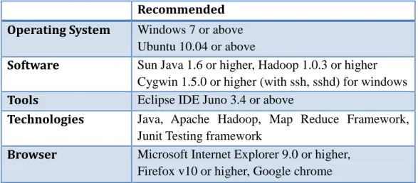
For a pseudo distributed mode we can use Windows 7 operating system with cygwin (includes ssh, sshd) or we can use Ubuntu 10.04 or above. Cygwin is required for windows so as perform the unix operations or linux like environment. The project requires hadoop environment with a stable version of Hadoop 1.x installed. To view logs and job tracker history a browser is needed.

Recommended Operating System Windows 7 or above

Ubuntu 10.04 or above

Software Sun Java 1.6 or higher, Hadoop 1.0.3 or higher Cygwin 1.5.0 or higher (with ssh, sshd) for windows Tools Eclipse IDE Juno 3.4 or above

Technologies Java, Apache Hadoop, Map Reduce Framework, Junit Testing framework

Browser Microsoft Internet Explorer 9.0 or higher, Firefox v10 or higher, Google chrome

(18)

- 11 -

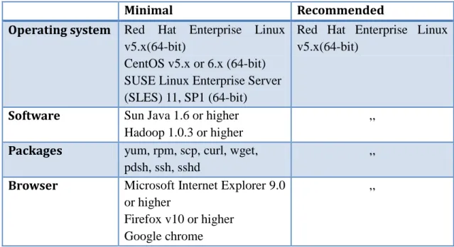
For this purpose Internet explorer 9.0 or above is preferable. Since hadoop is a java based system, the operating system should have java installed with Sun Java 1.6 or above. To execute on a server, a robust operating system like Red Hat Enterprise Linux (RHEL) v5.x (64-bit) is preferred. The Table 2.3.1.1 gives the software requirements for pseudo-distributed mode and Table 2.3.1.2 gives the software requirements for fully-distributed mode.

Minimal Recommended

Operating system Red Hat Enterprise Linux v5.x(64-bit)

CentOS v5.x or 6.x (64-bit) SUSE Linux Enterprise Server (SLES) 11, SP1 (64-bit)

Red Hat Enterprise Linux v5.x(64-bit)

Software Sun Java 1.6 or higher Hadoop 1.0.3 or higher

,, Packages yum, rpm, scp, curl, wget,

pdsh, ssh, sshd

,, Browser Microsoft Internet Explorer 9.0

or higher

Firefox v10 or higher Google chrome

,,

Table 2.3.1.2 Software Requirements - Fully Distributed mode

2.3.2 Hardware Requirements

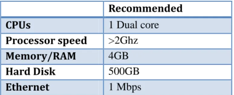
A pseudo distributed mode computing may not be capable of utilizing all the cores of a processor. There is no need for a high end hardware configuration as it is mostly used for developing and debugging the code. For a pseudo distributed mode a normal hardware configuration like dual core processor with 4 GB RAM and 500GB hard disk with processor speed of 2 GHz would be sufficient. In a fully distributed mode there are different types of processing environments like light weight, balanced and heavy computation. Each of them has different hardware requirements. For light weight processes a hardware configuration with 2 quad cores and 8GB RAM with 1Gbps Ethernet would be sufficient. For a balanced and heavy weight processes 2 quad core processors with 16-24GB RAM and 2Gbps Ethernet is required. The Table 2.3.2.1 gives the hardware requirements for the pseudo-distributed mode and Table 2.3.2.2 gives the hardware requirements for the fully-distributed mode.

(19)

- 12 -

Recommended

CPUs 1 Dual core

Processor speed >2Ghz

Memory/RAM 4GB

Hard Disk 500GB

Ethernet 1 Mbps

Table 2.3.2.1 Hardware Requirements - Pseudo Distributed mode

Minimal Recommended

CPUs 2 Quad core 2 Quad core

Processor speed >2Ghz >2Ghz

Memory/RAM 8GB 16-24GB

Hard Disk 4 disk drives(1 TB) 4 disk drives(2 TB)

Ethernet 1Gbps >2Gbps

Table 2.3.2.2 Hardware Requirements - Fully Distributed mode

2.4 Technologies Description

2.4.1 Hadoop Software Framework

Hadoop is an Apache Software Foundation project. It is an open source framework written in java for handling large scale distributed applications. It is used for developing and running data intensive distributed applications on large commodity clusters [1]. It is designed to handle large number of servers with high degree of fault tolerance. It is composed of mainly composed of two main components. They are Hadoop Distributed File System (HDFS) and Map Reduce computational model. It can process vast amount of data on an order of magnitude of petabytes which is larger than the existing systems. There have been lot of existing systems performing computation on large volumes in a distributed environment, but what unique about hadoop is that it has got a simplified programming which makes the programmers to develop and test the code for distributed applications easily. It is very efficient, distributes the work and data across different processing machines automatically. It fully utilizes the parallel computing power of the processing machines CPUs.

(20)

- 13 -

2.4.2 Hadoop Distributed File System

Hadoop Distributed File System (HDFS) can store large files across different machines in a reliable and efficient manner. It handles fault tolerance, network errors and provides high throughput. It has master/slave architecture with one single master ‘Namenode’ managing namespace, file access and several worker ‘Data nodes’. It splits the large data files into small size chunks, each managed by different nodes of the cluster. Data is replicated across several machines so that in the event of individual machine failure data will be still available. All these chunks are stored under a single namespace. As the files are spread across different machines as chunks, each node operates on a part of the data. This alleviates the burden of network transfers there by achieving high data locality, high performance and throughput.

Figure 2.4.2 Datanode and Namenode managing files in the form of blocks [9]

2.4.3 Hadoop Map Reduce Framework

Hadoop map reduce framework is a programming model designed to process large volumes of data in parallel. It runs only those programs which conform to the map reduce programming model. It has two phases of execution: mapping phase and reducing phase. Each phase has an input and output data set of key and value pairs. In the mapping phase, it splits the input data into a large number of data fragments and distributes them across different machines.

(21)

- 14 -

Figure 2.4.3.1 Distribution of data across different nodes [9]

Figure 2.4.3.2 Map Reduce pipeline on different nodes [9]

Each data fragment is assigned a map task. All the map tasks are executed in parallel which takes the input data and transforms them into set of intermediate key/value pairs using a user defined function. After this phase the intermediate values are sorted, merged and distributed into different fragments across different machines depending on the number of reducers and presented as input

(22)

- 15 -

to the reducing phase. Each fragment is assigned a reduce task which processes the data fragment into output key/value pairs depending on the user defined function. The output data of reducing phase is stored to the local machine. The map reduce framework consists of different nodes with a master/slave architecture having single master Jobtracker node and several slave Tasktracker nodes. All the map reduce jobs are added to the queue of pending jobs managed by Jobtracker. Jobtracker handles the entire map-reduce tasks and assigns them to the task trackers which execute tasks according to the instructions.

Figure 2.4.3.3 Internal Structure of Map Reduce data flow [9]

Hadoop implicitly handles the communication from node to node there by making it reliable. It tags the data fragments with key names so that it knows how to send data to the common destination node. It manages the data transfer and cluster configuration internally. It is very

(23)

- 16 -

robust when concerned with the data congestion issues. In the case of a node failure it restarts the tasks on other processing machines.

Hadoop has some disadvantages like the input data elements cannot be updated. It does not provide any security model or safe guards. As it consumes some time to start the map reduce tasks it may not show optimal performance with a small quantity of data processed over a small number of nodes.

2.5 Why Hadoop?

There are several existing softwares for distributed computing like MPI, CUDA and Apache Pig but they do not fit into criteria of the current project. The below discussion tell us why Hadoop is chosen for this project.

MPI consists of a message passing model. The threads of mpi system are independent to one another. The communication between all the machines is done through message passing over the network. The current project includes processing large number of small elements. If the MPI approach is used for the current project it uses a high amount of network bandwidth and very low CPU utilization which is not ideal.

CUDA is distributed computing software where it uses GPU for its computation. It is implemented using SMT paradigm. The execution of instructions is similar to the SIMD model. Here the amount of global memory and shared memory used in a GPU are limited. The current project consists of processing a large network graph which may not fit into the memory. Since the instructions are executed in a lock step fashion it may block the resource which is not ideal. For this reason CUDA is not used in the current project.

Apache Pig is highly scalable distributed computing software developed on hadoop map/reduce fundamentals. It reduces the lines of code need to be written for map/reduce jobs It uses data flow operations and creates a series of map reduce jobs for them automatically. The current project prototype does not fit here since the executions are done in a non-serializable fashion and most of the computations get repeated. It cannot check the convergence. The graph algorithms with Pig are generally very slow.

When compared with the above technologies Hadoop map-reduce use parallel tasks execution with different phases and has convergence of all the intermediate results between each map and reduce job. This is ideal and required for the current project.

(24)

- 17 -

2.6 Discussion – Other approaches

There are several algorithms developed for computing the all pairs shortest path problem. Most of these algorithms are designed from two basic algorithms: Dijkastras algorithm [4] and Floyd-Warshall Algorithm [3]. Dijkastras algorithm solves for shortest path from single source to all other vertices. This can be used for computing APSP problem by iterating it over all the vertices. The Floyd-Warshall algorithm solves for the APSP problem by saving the computed shortest distance of intermediate paths for each pair at each step. The following discussion presents some of the approaches developed for solving the Parallel APSP problem in distributed mode. The discussion uses the term ‘relax’ to specify the shortest path calculation for a single graph node.

2.6.1 Parallel Dijkastras APSP

A Parallel Dijkastras APSP computation is done by executing each Single source shortest path on each of the processors. For this approach, the adjacency matrix is to be replicated on to all the processors. This approach supposes that there are enough processors, one for each node. The execution is done in an independent fashion with no much of inter process communication between processors. It takes same time as that of computing it for Single source shortest path SSSP. This has a run time complexity of O(n2), with a given ‘n’ number of vertices.

Another version of Parallel Dijkastras scheme [8] is to partition the number of vertices and execute each partition on a separate processor. In distributed mode for a given p processors, each of SSSP is executed on the n/p processors. The nodes in each partition uses Dijkastras algorithm to solve for the shortest path. It has a time complexity of O(n3/p)+O(n log p).

The speed ups for these two versions are almost equal to ‘p’. The pros of this approach are optimal time complexity; low bandwidth, easy to compute, no underlying complexity involved and no inter process communication whereas the cons are: it requires the number of processors equal to the number of vertices, no node level parallelism and adjacency matrix should be replicated on each of the processors.

2.6.2 Simple Parallel Floyd Warshall APSP

The Simple Parallel Floyd Warshall APSP [7] scheme uses the Floyd Warshall algorithm. In this scheme, the initial adjacency matrix is distributed among different processors each sharing some portion of the rows like 1..k of the initial adjacency matrix rows of 1..n, where 1<k<n. Each

(25)

- 18 -

processor owning a row 'k' broadcasts the whole row over the network to the other processors. Each processor receives rows broadcasted by other processors and relaxes them with the rows owned by them. In this cost of communication depends on broadcast latency, bandwidth and time taken to relax single entry. For a given ‘p’ processors and ‘n’ number of vertices, the time complexity of this scheme is O(n3/p)+O(n2)+O(n).

The pros of this scheme are low bandwidth, good load balancing and efficient CPU utilization. The cons of this scheme are poor cache performance, requires matrix representation of graph in heap memory.

2.6.3 Blocked Floyd Warshall APSP

The Blocked Floyd Warshall APSP [5] scheme considers the adjacency graph is partitioned into blocks. If ‘n’ is the size of the matrix and ‘b’ is the size of the block, then the number of blocks is

N2, where N=n/b. For this algorithm if there are ‘p’ cluster nodes, then the block size is b=n/p. Each cluster node is assigned one complete row of blocks.

In this approach processors broadcast their pivot row blocks over the network. Each processor receives and computes pivot row block and pivot column block sent by other processors and relax their own pivot blocks and then other non-pivot blocks. The relaxing of blocks is done in an order. It then broadcasts them for the next iteration.

This approach has a time complexity of O(n3/p)+O(n2). The pros of this approach are low bandwidth, good load balancing and efficient CPU utilization. The cons of this approach are computation is complex, needs adjacency matrix representation of graph, no failure recovery methods, inefficient for medium sized graphs and nodes have to wait for the relaxation step and till the broadcast of the next iteration.

2.6.4 Parallel Map Reduce APSP

This is the current algorithm used in our project. It is done in two phases: Building Adjacency Graph and Running Parallel APSP Map Reduce. In the first phase of building adjacency graph, adjacency list with trio sets are created from the input links. In the next phase of running parallel apsp map reduce, the algorithm makes use of the adjacency list representation of the graph in a specific format. Each node is represented using adjacency list and trio sets. Each Trio set for a node consists of the destination node, shortest distance to the destination node and color to check

(26)

- 19 -

if the destination node is visited or unvisited. The process involves a Map phase and a Reduce phase iterated over a Stopping condition.

The map phase consists of processing all the nodes with the ALTS format. For each node it checks if there is any trio set with an unvisited color. It sets the stopping condition flag to false. It emits the original source node as key and the trio set with color changed to visited color. It also emits each of the adjacent nodes of original source node as key and the trio set with distance increased by '1' in it. This process of mapping continues until the stopping condition is true. In the reducer phase, the nodes that are emitted by the mapper phase are continued. For each node emitted by the Mapper, the values of the trio sets are checked for least distance and darkest color of the destination node and the list of triosets for each node are updated. This process of map reduce iterations continues until the stopping condition is set to true.

For a graph with size ‘n’, M mappers, R reducers and T threads for each map/reduce task. The Buidling Adjacency Graph phase has a time complexity of O(n2/MT)+O(n2/RT) and Running Parallel APSP Map Reduce phase has a time complexity of O(n3/MT)+O(n3/MT). For a given system with ‘p’ number of processors MT >> p, RT >> p i.e., MT and RT values are much greater than ‘p’. This implies that the current algorithm has the best time complexity when compared to other existing approaches. For an average case, assuming the longest shortest path will be a constant ‘k’ << ‘n’, the average time complexity will be O(n2/MT)+O(n2/RT). This shows that the system can perform in an order of ‘n2’ time complexity for average case, which is the least time complexity when compared to that of existing systems.

The pros of this approach are mapper phase has an efficient CPU utilization when compared to other existing systems, fault tolerant, optimal time complexity, provides node level parallelism, good load balancing, high throughput and less inter process communication.

The cons of this approach are reducer phase has to wait till all the intermediate values are sorted and merged, requires hadoop cluster system environment, initialization of map reduce tasks take time.

(27)

- 20 -

Chapter 3 - Implementation

Before we implement the system we try to develop a pseudo code and understand the working of it; we try to devise a plan and implement it accordingly to develop the system. The following section discusses about the pseudo code and working for the two algorithms developed for this project.

The following Sample graph shown in Figure 3.1 with 5 nodes is used to describe the working of the two algorithms.

Figure 3.1 Sample 5-Node Graph

3.1 Modules

The project is implemented in two main modules. They are Build Adjacency Graph from the given network data and running Parallel APSP Map Reduce on the Adjacency Graph.

3.1.1 Build Adjacency Graph

The “Build Adjacency Graph” module includes extracting the links from the network data file, transforming the links into adjacency list, formatting the output by adding default trio set and writing it to a file. The users and their links are extracted from the file. The extracted user pairs are then joined with the first user as the key and the list of users attached to the user as adjacency

(28)

- 21 -

list separated by a tab. The process of extraction and transformation uses the map reduce paradigm which processed all the links in parallel in mapper phase. The reducer phase waits for the completion of mapper phase and formats the adjacency list derived. The output graph format will have the information for both the in-links and reachable nodes from out-links.

Pseudo code for Building Adjacency Graph

The following Figure 3.1.1 gives the Pseudo code for Building Adjacency Graph module.

Figure 3.1.1 Pseudo code - Building Adjacency Graph

(29)

- 22 -

Working

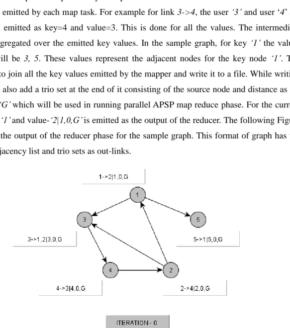
The input for this algorithm is the sample network graph data shown in Figure 3.1.1.1 which consists of friendship links separated by a ‘separator’. The user1 and user2 from each link are extracted and emitted by each map task. For example for link 3->4, the user ‘3’ and user ‘4’ are

extracted and emitted as key=4 and value=3. This is done for all the values. The intermediate values are aggregated over the emitted key values. In the sample graph, for key ‘1’ the values aggregated will be 3, 5. These values represent the adjacent nodes for the key node ‘1’. The reducer tries to join all the key values emitted by the mapper and write it to a file. While writing it to a file we also add a trio set at the end of it consisting of the source node and distance as ‘0’ and color as ‘G’ which will be used in running parallel APSP map reduce phase. For the current example key-‘1’ and value-‘2|1,0,G’ is emitted as the output of the reducer. The following Figure 3.1.1.2 gives the output of the reducer phase for the sample graph. This format of graph has the in-links as adjacency list and trio sets as out-links.

Figure 3.1.1.2 Output Graph of Building Adjacency Graph using Map Reduce

Time Complexity

The time for processing the Mapping phase consists of initializing the map tasks and processing all the mappers in parallel. Considering there are a total of nm tasks in the mapping phase with M number of map tasks and T number of threads per each task. Let tim be the time taken to initialize

(30)

- 23 -

a single mapper. The total time taken to initialize all the map tasks would be Mtim. Apart from the initialization of map tasks the time taken to process the whole mapping phase will depend on the time taken to process each single map task. Each mapper consists of nm/M tasks. If tm is the time taken to process each single task, the time taken for a single mapper execution will be nmtm/M. As each map task has ‘T’ threads processing it, the time taken will be nmtm/MT. Since all the mappers are processed in parallel the total time for all the mappers will also be nmtm/MT. Let TM be the total time for the mapping phase then

TM = Mtim + nmtm/MT The Reducer is also processed in a similar fashion.

TM = Rtir + nrtr/RT The total time taken for building adjacency graph

TBAG = TM + TR = Mtim + nmtm/MT + Rtir + nrtr/RT

The time complexity is of order of O(nmtm/MT) + O(nrtr/RT). For a given graph with ‘n’ number of nodes, nm will be of the order of O(n2). So, the worst case time complexity of Building Adjacency Graph will be O(n2/MT)+O(n2/RT).

3.1.2 Running Parallel APSP Map Reduce

The “Running Parallel APSP Map Reduce” module includes the process of running parallel APSP Map reduce algorithm through iterative phases and calculating the BDD for all pairs of nodes in the network graph. The algorithm is iterated by checking a Boolean flag called stopping condition which determines if there is any next iteration. All the iterations consist of a mapper phase and a reducer phase. The mapper phase includes extracting the trio sets from each node, processing them by their color and distance, sending it to the reducer. The reducer phase tries to evaluate the key value pairs of trio sets emitted by the mapper and process them by checking for least distance and darkest color so as to keep the concept of shortest distance from source node to destination node. The processed nodes are used as input for the next iteration. The process continues until all the nodes are explored and all possible shortest paths are computed.

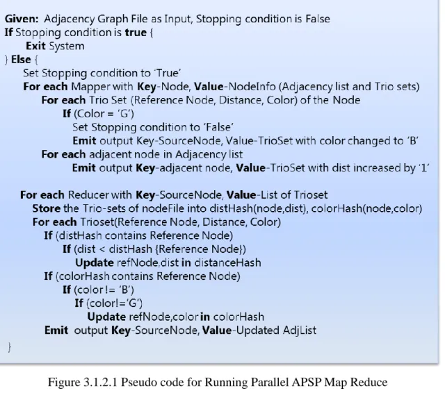
Pseudo code for Running Parallel APSP Map Reduce

The following Figure 3.1.2.1 gives the Pseudo-code for the Running Parallel APSP Map Reduce module.

(31)

- 24 -

Figure 3.1.2.1 Pseudo code for Running Parallel APSP Map Reduce

Working

The algorithm requires an adjacency list with trio sets format as input and stopping condition set to false. In the initial step the adjacency list file is the output of the Building Adjacency Graph module. It checks for the global variable ‘Stopping condition’ at the starting of iteration. If the variable is ‘true’ then it exits the system without processing further. If it is ‘false’, then it enters into the iteration. Each iteration consists of a map phase and a reduce phase. In the map phase, the mappers process all the lines with node information in parallel. Each mapper splits the input node information line into adjacency list and trio sets. It checks if there exists color ‘G’ in any of the trio sets and updates the Stopping condition variable to ‘false’. The color ‘G’ is used to represent the information that the node can be processed further in the next iteration. The trio sets for a source node represent the information of other reference nodes from which it can be

(32)

- 25 -

reached. The trio sets are generated at the node with the adjacency list and source node. In each iteration they are sent to the connected nodes thereby making the trio sets travel from source node to all of its connected reference nodes one level/hop at a time. In the process of travelling from one node to other connected nodes, the triosets for a node are updated which gives the information of shortest distance from a reachable node to the source node. After the completion of all the iterations, each source node will be having the connected reference node information in the form of trio sets. At last the shortest distances for all the nodes are calculated at the end of iterations.

In the current example, the stopping condition variable is set to ‘false’ before the starting of the algorithm so that it can enter into the iteration loop. For the node ‘1’ it consists of trio set

(1,0,G) which has color ‘G’. It sets the stopping condition to false. It then emits the source node

‘1’ and trio set (1,0,B). This is to acknowledge that trio set with reference node ‘1’ is processed by current map task. It then emits the adjacent nodes as key and the value as trio set (1,1,G). This tells us that the node ‘1’ information is sent to the connected nodes which are the adjacent nodes of the source node and the adjacent nodes will be having the node ‘1’ with distance ‘1’ and color

‘G’. The outputs emitted for node’1’ after the first map phase with key-value pairs are :(1 1,0,B)

and (2 1,1,G). In the reducer phase, the node ‘2’ receives the trio set (1,1,G) and updates its triosets list. It first checks if the trioset received is having the least distance than the existing trioset for reference node ‘1’ in trio set. It then checks for the darkest color and update its corresponding trioset. Similarly all the nodes update their triosets list. In the next iteration i.e., Iteration-1, node 1 and node 2 processes the triosets received from the previous iteration. For node ‘1’, it has (1,0,B), (3,1,G), and (5,1,G). It checks the color of each trioset and it forwards triosets with ‘3’ and ‘5’ to its adjacent node ‘2’ as they have their color ‘G’. The values emitted for node ‘1’ are (1 3,1,B), (2 3,2,G), (1 5,1,B) and (2 5,1,G). In the reducer phase each node receives the triosets forwarded by other nodes and updates their triosets list. In this way the information for received by node ‘1’ is forwarded to it in-link nodes at each iteration. All the nodes are processed in the same manner. The process continues for several iterations until there are no trio sets with color ‘G’ encountered. At last the node ‘1’ will have the triosets (3,1,B), (5,1,B), (4,2,B) and (2,3,B) representing all the reachable nodes from it. The following figures give the adjacency list with trio sets and key/value pairs emitted for all the iterations.

(33)

- 26 -

Figure 3.1.2.2 Iteration-0 Graph - Running Parallel APSP Map Reduce

(34)

- 27 -

(35)

- 28 -

Time Complexity

The time complexity for this algorithm depends on tasks of map-reduce phases and the number of iterations of map-reduce phases. Consider there are a total number of nm tasks in the map phase and M mappers with T number of threads for each map task. Let tim be the time taken to initialize a single mapper. The total time taken to initialize all the map tasks would be Mtim. The

(36)

- 29 -

time taken to compute a single task depends on the time taken to process the trio sets. Let nmt be the number of trio sets processed for each task and tmt is the time taken to process it. The time taken for a single task is nmttmt. The time taken to execute all the tasks in map phase is

nmnmttmt/MT. The total time for the mapping phase will be

TM = Mtim + nmnmttmt/MT Similarly the time taken for the Reduce phase is

TR = Rtir + nrnrttrt/RT

The total time taken for running the Parallel APSP Map Reduce algorithm is

TPAPSP = I (TM + TR) = I (Mtim + nmnmttmt/M + Rtir + nrnrttrt/R), where ‘I’ is the number of iterations. The Total Time complexity for Running Parallel APSP Map Reduce is

O(nmnmttmtI/MT)+O(nrnrttrtI/RT). The ‘I’ value represents the longest shortest path and in worst case it could be ‘n’. In worst case the number of triosets and number of tasks will be in an order of ‘n’. So, the worst case time complexity of the algorithm is O(n3/MT)+O(n3/RT). If we consider an average case, number of triosets and number of tasks will be in an order of log n. So, the average time complexity of the algorithm will be O(n*(log n)2/ MT)+O(n*(log n)2/RT).

3.2 Coding

The coding of the system is done using four different class files: GraphBasesFeaturesTrain, Graph, Variables and Stopwatch. The first java class file GraphBasesFeaturesTrain is actual java class file in which the friendship prediction for the input social network is done using GBF features and BDD calculation. The two other java files were developed to implement the Building adjacency graph and Running parallel APSP map reduce algorithms. Variables and Stopwatch are supporting classes used in other classes.

GraphBasesFeaturesTrain - In GraphBasesFeaturesTrain.java class file, a string variable ‘mainDir’ is used to set the main folder path, which will be used as the working folder. Using this main directory path other directory paths are set and organized which are used in the further processes. In the map reduce execution the class instance variables get destroyed when they are used for the next phase or iteration. To overcome this problem, the global variables are maintained in the form of files under a directory named ‘variables’. The folder ‘In’ is used as input for building the adjacency graph process. The output adjacency graph will be stored in the directory called ‘Out’ having file for each node. The folder also contains a combined file which

(37)

- 30 -

is used as input for the parallel APSP mapreduce process. The process updates the ‘Out’ folder files after each iteration and combines all the files into a single file and uses the file as input for the next iteration.

Graph - The Graph.java class file contains methods to check and organize the directory structure of the file system, map reduce methods for building adjacency graph and running parallel APSP.

Varibles - The Variables.java class file contains methods to set and get the variables, folder paths. These methods are used by the other two java classes. The various variables that are set and used in the class files are mainDir, dataDir, graphDir, inputDir, inputTrainDir, outputDir, outputTrainDir, tempDir, outputTrainFile and stoppingCondition. Of all these variables

stoppingCondition is checked at the start of each iteration to check whether there is need to process for the next iteration.

Stopwatch - The Stopwatch.java class file is created to record the amount of time taken for the execution. It contains a method getelapsedTime, which returns the elapsed time since from the starting time.

Text data format is used as the input data format & output data format for the map and reduce phases for both the methods of building adjacency graph and running parallel APSP. The Text Format is used here because of its simplicity and easiness of conversions to other formats.

(38)

- 31 -

3.3 Diagrams

3.3.1 Class Diagram

Figure 3.3.1 Class Diagram

The Figure 3.3.1 represents the class diagram for the current system. It shows how the system is organized. The diagram shows that the GraphBasedFeaturesTrain class uses the Graph and Variables classes; Graph class uses Variables class and has a Stopwatch class object. It shows that the system is organized under the package ‘hadoopParallelAPSP’.

(39)

- 32 -

3.3.2 Data Flow Diagrams

Figure 3.3.2.1 Context Level Diagram

The Figure 3.3.2.1 represents the Context Level Diagram for the current system. It shows that different modules of extracting network data, building adjacency graph and running parallel APSP map-reduce.

Figure 3.3.2.2 Level-0-DFD - Extracting network data and generating instances

The Figure 3.3.2.2 represents Level-0-DFD for Extracting Network data and generating instances activity. It shows that the social network data is taken as input and links from network data are extracted and stored. The Train data is then compared with stored links to check whether they exist. The existing links from train data are used for generating instances.

The Figure 3.3.2.3 represents the Level-0-DFD for Building the Adjacency Graph mod-ule. It shows that the input links from the GraphBasedFeaturesTrain are formatted and sent to the Building Adjacency Graph mapper. The Building Adjacency Graph Reduce phase uses the inter-mediate values to build the trioset formatted Adjacency Graph.

(40)

- 33 -

Figure 3.3.2.3 Level-0-DFD - Building Adjacency Graph

Figure 3.3.2.4 Level-0-DFD - Running Parallel APSP Map Reduce

The Figure 3.3.2.4 represents the Level-0-DFD for Running Parallel APSP Map Reduce module. The diagram shows that trioset formatted adjacency graph is used as input. In mapping phase stopping condition is checked and triosets of adjacency list are processed according to dis-tance and color. In the reducing phase intermediate values are merged and triosets are updated for each node. The updated adjacency list with triosets is given as input for the next iteration.

(41)

- 34 -

Chapter 4 - Evaluation

4.1 Testing

Once the application is developed, it needs to be tested to make sure the application meets all the functional requirements for which it was designed for. Testing is classified mainly into two types. They are Black Box Testing and White Box Testing. Black Box Testing involves testing the system for different types of external inputs and its behavior. In this testing the internal structure of the system is not known to the tester. It includes different types of testing like Load Testing, Performance Testing, System Testing and Acceptance Testing. For the current project Performance Testing and System Testing are used. White Box Testing involves testing the internal structure and implementation of the system. In this testing the internal units of the system are rigorously tested for all kinds of valid and invalid inputs, all logical paths, conditional statements and loops. It determines how well the system behaves and also gives an overview of integrity of the system. It includes different types of testing like Unit Testing and Integration Testing. Unit testing is used for the current project.

4.2 Test Methods & Test plan

4.2.1 Unit Testing

As the current system is developed in java we have used JUnit for unit testing the system. JUnit is a testing framework for writing test cases and unit testing java applications. It has a Text Fixture java object for setting the test environment and Test Case java object for writing and testing different test cases. We try to check for the correctness of the system by unit testing it for various test cases. We test the system to check if it is returning the correct output for different types of graphs, if the paths and variables are preserved correctly at each phase, if it tries to check for the invalid data format. We also check if it is preserving the stopping condition correctly at each and every phase. The directed graphs with graph size 5 and 10 nodes are used in this testing. The unit testing considering testing the system for both the types of graphs of cyclic graphs and acyclic graphs. The below Table 4.2.1 shows different test cases used for unit testing the system.

(42)

- 35 -

Test No.

Initial State Test Case Expected Result

1 Connected cyclic graph with size 5

Compare output shortest paths of parallel Map Reduce APSP with pre-calculated shortest paths.

Success: Output Results match the pre-calculated shortest paths.

,, ,,

3 Disconnected cyclic graph with size 5

,, ,,

4 Disconnected cyclic graph with size 10

,, ,,

5 Connected Acyclic graph with size 5

,, ,,

6 Connected Acyclic graph with size 10

,, ,,

7 Disconnected Acyclic graph with size 5

,, ,,

8 Disconnected Acyclic graph with size 10

,, ,,

Check if the system preserves the input and output directory path variables

Success: Yes it preserves the input and output path variables

Check if the stopping condition is set correctly

Success: Yes the stopping condition set.

11 Connected cyclic graph with size 10 (invalid data format)

Check if the input data format is valid or invalid.

Exception: Input has invalid data format

(43)

- 36 -

Figure 4.2.1 Test Results for Unit Testing

The above diagram Figure 4.2.1 shows the results for the Unit Testing. It tells us that the system has passed the entire unit testing test cases successfully.

4.2.2 Performance Testing

The System is tested for performance testing to analyze different factors like scalability, efficiency and speedups. It gives us an idea of responsiveness of the system under a given work load. In order to judge the true parallel computing capability of the system, we try to test for its performance using inputs of different data sizes. The graphs with sizes from 50 nodes to 1,000,000 nodes are taken as input for measuring the performance of the system with number of cores ranging from 2 to 16 cores. The Table 4.2.2 gives us the performance testing results.

(44)

- 37 -

Table 4.2.2 Test Results of Performance Testing

Figure 4.2.2 Line Graph representing Performance Testing Results

General Floyd Warshall

APSP

Building Running Longest

Adjacency Parallel Map Reduce Shortest

Graph APSP Path

50 0.278 3.65 24.968 28.618 8 2 Cores 4GB RAM 500 0.775 16.193 146.944 163.137 23 2 Cores 4GB RAM 1000 4.829 26.598 147.063 173.661 17 4 Cores 8GB RAM 5000 236.443 80.87 343.943 424.813 9 4 Cores 8GB RAM 10000 1370.771 172.516 1169.063 1341.579 19 4 Cores 8GB RAM 20000 2656.631 146.794 1955.428 2102.222 12 4 Cores 8GB RAM 30000 11621.479 214.312 1563.712 1778.024 8 4 Cores 8GB RAM 50000 40735.363 396.489 1672.237 2068.726 8 4 Cores 8GB RAM 100000 238.056 1029.256 1267.312 8 4 Cores 8GB RAM 200000 135.498 623.317 758.815 8 8 Cores 16GB RAM 500000 332.677 1244.931 1577.608 8 8 Cores 16GB RAM 1000000 201.361 890.544 1091.905 8 16 Cores 32GB RAM 200000 469.399 1774.103 2243.502 8 4 Cores 8GB RAM 500000 592.262 2149.402 2741.664 8 4 Cores 16GB RAM 1000000 670.386 3314.856 3985.242 8 4 Cores 32GB RAM 1000000 330.402 1882.528 2212.93 8 8 Cores 32GB RAM

Parallel Map Reduce APSP

Graph Size Total Time # Cores / RAM

1 2 4 8 16 32 64 128 256 512 1024 2048 4096 8192 16384 32768 Exec u tion Ti m e ( Se cs)

Graph Size (#Nodes)