ApproxHadoop: Bringing Approximations
to MapReduce Frameworks
´I˜nigo Goiri
†∗Ricardo Bianchini
†‡Santosh Nagarakatte
‡Thu D. Nguyen
‡ ‡Rutgers University
†Microsoft Research
{
ricardob, santosh.nagarakatte, tdnguyen
}
@cs.rutgers.edu
{
inigog, ricardob
}
@microsoft.com
Abstract
We propose and evaluate a framework for creating and run-ning approximation-enabled MapReduce programs. Specif-ically, we propose approximation mechanisms that fit nat-urally into the MapReduce paradigm, including input data sampling, task dropping, and accepting and running a pre-cise and a user-defined approximate version of the MapRe-duce code. We then show how to leverage statistical theories to compute error bounds for popular classes of MapReduce programs when approximating with input data sampling and/or task dropping. We implement the proposed mech-anisms and error bound estimations in a prototype system called ApproxHadoop. Our evaluation uses MapReduce ap-plications from different domains, including data analytics, scientific computing, video encoding, and machine learning. Our results show that ApproxHadoop can significantly re-duce application execution time and/or energy consumption when the user is willing to tolerate small errors. For exam-ple, ApproxHadoop can reduce runtimes by up to32×when the user can tolerate an error of 1% with 95% confidence. We conclude that our framework and system can make ap-proximation easily accessible to many application domains using the MapReduce model.
Categories and Subject Descriptors C.4 [Computer Sys-tems Organizations]: Performance of SysSys-tems; D.m [Soft-ware]: Miscellaneous
Keywords MapReduce, approximation, multi-stage sam-pling, extreme value theory
∗This work was done while ´I˜nigo Goiri was at Rutgers University.
Permission to make digital or hard copies of all or part of this work for personal or classroom use is granted without fee provided that copies are not made or distributed for profit or commercial advantage and that copies bear this notice and the full citation on the first page. Copyrights for components of this work owned by others than the author(s) must be honored. Abstracting with credit is permitted. To copy otherwise, or republish, to post on servers or to redistribute to lists, requires prior specific permission and/or a fee. Request permissions from [email protected].
ASPLOS ’15, March 14–18, 2015, Istanbul, Turkey..
Copyright is held by the owner/author(s). Publication rights licensed to ACM. ACM 978-1-4503-2835-7/15/03. . . $15.00.
http://dx.doi.org/10.1145/2694344.2694351
1.
Introduction
Motivation. Despite the enormous computing capacity that has become available, large-scale applications such as data analytics and scientific computing continue to ex-ceed available resources. Furthermore, they consume sig-nificant amounts of time and energy. Thus, approximate computing has and continues to garner significant attention for reducing the resource requirements, computation time, and/or energy consumption of large-scale computing (e.g., [5, 6, 10, 17, 38]). Many classes of applications are amenable to approximation, including data analytics, machine learn-ing, Monte Carlo computations, and image/audio/video pro-cessing [4, 14, 25, 30, 41]. As a concrete example, Web site operators often want to know the popularity of individual Web pages, which can be computed from the access logs of their Web servers. However, relative popularity is often more important than the exact access counts. Thus, esti-mated access counts are sufficient if the approximation can significantly reduce processing time.
In this paper, we propose and evaluate a framework for creating and running approximation-enabled MapReduce programs. Since its introduction [13], MapReduce has be-come a popular paradigm for many large-scale applications, including data analytics (e.g., [2, 3]) and compute-intensive applications (e.g., [15, 16]), on server clusters. Thus, em-bedding a general approximation approach in MapReduce frameworks can make approximation easily accessible to many applications.
MapReduce and approximation mechanisms.A MapRe-duce job consists of user-provided code executed as a set of map tasks, which run in parallel to process input data and produce intermediate results, and a set of reduce tasks, which process the intermediate results to produce the final results. We propose three mechanisms to introduce a gen-eral approximation approach to MapReduce: (1)input data sampling: only a subset of the input data is processed, (2) task dropping: only a subset of the tasks are executed, and (3)user-defined approximation: the user provides a precise and an approximate version of a task’s code. These
mecha-nisms can be easily applied to a wide range of MapReduce applications (Section 5).
Computing error bounds for approximations.Critically, in Section 3, we show how multi-stage sampling theory [27] and extreme value theory [11] can be used to compute error bounds (i.e., confidence intervals) for approximate MapRe-duce computations. Specifically, we apply the former theory to develop a unified approach for computing error bounds when using input data sampling and/or task dropping in ap-plications that use a set of aggregation (e.g., sum) reduce op-erations. We apply the latter theory to compute error bounds when using task dropping in applications that use extreme value (e.g., min/max) reduce operations. Such error bounds allow users to intelligently trade accuracy to improve other metrics (e.g., performance and/or energy consumption).
ApproxHadoop.We have implemented our proposed mech-anisms and error bound estimations in a prototype system called ApproxHadoop, which we describe in Section 4. (In this paper, we limit our discussions to the first two mech-anisms, input data sampling and task dropping, because of space constraints. The description and evaluation of user-defined approximation can be found in our longer technical report [19].) For MapReduce programs that use Approx-Hadoop’s error estimation, the user can specify the desired error bounds at a particular confidence level when submit-ting a job. As the job is executed, ApproxHadoop gathers statistics and determines a mix of task dropping and/or input data sampling to achieve the desired error bounds. Alterna-tively, the user can explicitly specify the fraction of tasks that can be dropped (e.g., 25% of map tasks) and/or the data sampling ratio (e.g., 10% of data items). In this case, ApproxHadoop computes the error bounds for the speci-fied levels of approximation. This second approach can also be used for running arbitrary ApproxHadoop programs that can tolerate approximations, but for which ApproxHadoop’s error-bounding techniques do not apply; of course, Approx-Hadoop cannot compute error bounds for such jobs.
Evaluation.We use ApproxHadoop to implement and study approximation-enabled applications in several domains, in-cluding data analytics, scientific computing, video encoding, and machine learning. In Section 5, we present represen-tative experimental results for some of these applications. These results show that ApproxHadoop allows users to trade small amounts of accuracy for significant reductions in ecution time and energy consumption. For example, the ex-ecution time of an application that counts the popularity of projects (subsets of articles) in Wikipedia from Web server logs for one week (217GB) decreases by 60% when the user can tolerate a maximum error of 1% with 95% confidence. This runtime decrease can be even greater for larger input
data (and the same maximum error and confidence); e.g.,
32×faster when processing a year of log entries (12.5TB). Our results also show that, for a wide range of error tar-gets, ApproxHadoop successfully chooses combinations of
data sampling and task dropping ratios that achieve close to the best possible savings whilealways achieving the target error bounds. For the same project popularity application, ApproxHadoop reduces the execution time by 79% when given a target maximum error of 5% with 95% confidence.
Contributions. In summary, we make the following con-tributions: (1) we propose a general set of mechanisms for approximation in MapReduce, (2) we show how statistical theories can be used to compute error bounds in MapReduce for rigorous tradeoffs between approximation accuracy and other metrics, (3) we implement our approach in the Approx-Hadoop prototype, and (4) via extensive experimentation with real systems, we show that ApproxHadoop is widely applicable to many MapReduce applications, and that it can significantly reduce execution time and/or energy consump-tion when users can tolerate small amounts of inaccuracy.
2.
Background
MapReduce.MapReduce is a computing model designed for processing large data sets on server clusters [13]. Each MapReduce computation processes a set of input key/value pairs and produces a set of output key/value pairs. Each
MapReduce program defines two functions: map() and
reduce(). The map()function takes one input key/value
pair and processes it to produce a set of intermediate key/-value pairs. Thereduce() function performs a reduction computation on all the values associated with a given inter-mediate key to produce a set of final key/value pairs.
A MapReduce computation is executed in two phases by a MapReduce framework, a Map phase and a Reduce phase. To execute the Map phase, the framework divides the input data into a set of blocks, and runs amap taskfor each block that invokes map() for each key/value pair in the block. To execute the Reduce phase, the framework first collects all the values produced for each intermediate key. Then, it partitions the intermediate keys and their associated values among a set ofreduce tasks. Each reduce task invokes
reduce() for each of its assigned intermediate key and
associated values, and writes the output into an output file. In practice, it has been observed that MapReduce
exe-cutions often take the form of waves of map and reduce
tasks, where most map/reduce tasks require similar amounts of processing time as each other [48]. We leverage this ob-servation later in our implementation of ApproxHadoop.
Hadoop.Hadoop is the best-known, publicly available im-plementation of MapReduce [1]. Hadoop comprises two main parts: the Hadoop Distributed File System (HDFS) and the Hadoop MapReduce framework. Input and output data to/from MapReduce programs are stored in HDFS. HDFS splits files across the local disks of the servers in the cluster.
A cluster-wide NameNode process maintains information
about where to find each data block. ADataNodeprocess at each server services accesses to data blocks.
The framework is responsible for executing MapReduce jobs. Users submit jobs to the framework using a client in-terface; the user provides configuration parameters via this interface to guide the splitting of the input data and set the number of map and reduce tasks. Jobs must identify all in-put data at submission time. The interface submits each job to theJobTracker, a cluster-wide process that manages job execution. Each server runs a configurable number of map and reduce tasks concurrently in compute slots. The Job-Trackercommunicates with theNameNodeto determine the location of each job’s data. It then selects servers to execute the jobs, preferably ones that store the needed data locally if they have slots available. Each server runs aTaskTracker process, which initiates and monitors the tasks assigned to it. TheJobTrackerstarts a duplicate of any straggler task,i.e.a task that is taking substantially longer than its sibling tasks.
3.
Approximation with error bounds
We propose three mechanisms for approximation in MapRe-duce: (1) input data sampling, (2) task dropping, and (3) user-defined approximation [19]. In this section, we use theories from statistics to rigorously estimate error bounds when approximating using input data sampling and/or task dropping.
3.1 Aggregation
Multi-stage sampling theory.We leverage multi-stage sam-pling [27] to compute error bounds for approximate MapRe-duce applications that compute aggregations (e.g., counting accesses to Web pages from a log file). The set of supported aggregation functions includessum,count,average, and ra-tio. For simplicity, we next discuss two-stage sampling. De-pending on the computation, it may be necessary to use addi-tional sampling stages as discussed at the end of the section. Two-stage sampling works as follows. Suppose we have a population of T units, and the population is partitioned into N clusters. Each cluster i contains Mi units so that
T =PN
i=1Mi. Suppose further that each unitjin clusteri
has an associated valuevij, and we want to compute the sum
of these values across the population,i.e.PN
i=1
PMi
j=1vij.
(We describe the approximation of sum in the remainder of the subsection; approximations for the other operations are similar [27].)
To compute an approximate sum, we can create a sample by randomly choosingnclusters, and then randomly choos-ingmiunits from each chosen clusteri. Two-stage sampling
then allows us to estimate the sum from this sample as:
ˆ τ= N n n X i=1 (Mi mi mi X j=1 vij)± (1)
where the error boundis defined as: =tn−1,1−α/2 q d V ar(ˆτ) (2) d V ar(ˆτ) =N(N−n)s 2 u n + N n n X i=1 Mi(Mi−mi) s2 i mi (3) where (s2
u) is the inter-cluster variance (computed using the
sum and average of the values associated with units from each cluster in the sample), (s2
i) is the intra-cluster variance
for clusteri, andtn−1,1−α/2 is the value of the Student
t-distribution withn−1 degrees of freedom at the desired confidence1−α. Thus, to compute the error bound with 95% confidence, we use the valuetn−1,0.975[27].
Applying two-stage sampling to MapReduce. To apply two-stage sampling to MapReduce, we associate population, clusters, and the value associated with each unit in the pop-ulation to the respective components in MapReduce. As an example, consider a program that counts the occurrence of a wordW in a set of Web pages, where the Map phase counts
the occurrence ofW in each page, and the Reduce phase
sums the counts. Suppose that the program is then run on an input data set withTpages (input data items), and the frame-work partitions the input intoNdata blocks. In this case, the population corresponds to theTpages, with each page being a unit. Each data blockiis a cluster, whereMiis the number
of units (pages) in the block. The Map phase would produce <W, vij>for each unit (page) j in cluster (data block)i,
wherevijis the value associated with that unit.
With the above associations, an approximate computation can be performed by executing only a subset of randomly chosen map tasks, using task dropping to avoid the exe-cution of the remaining map tasks. Further, each map task only processes a subset of randomly chosen pages (input data items) from its data block using input data sampling. Together, these actions are equivalent to choosing a sample using two-stage sampling. Thus, in the Reduce phase, Equa-tions 1 and 2 can be used to compute the approximate sum and error bounds.
For jobs that produce multiple intermediate keys, we view the summation of the values associated with each key as a distinct computation. As an example, consider a program that counts the occurrence of every word that appears in a set of Web pages. The Map phase now produces a set of counts for each word appearing in the input pages. Assuming there arezwords, Equations 1 and 2 are used in the Reduce
phase to produce z approximate sums, each with its own
error bound.
Figure 1 illustrates an approximate computation that pro-duces several final keys and their associated sums. In this computation, the sample comprises the 2nd and 4th input data items from block 1, all data items from block 2, the 1st,
3rd, and 5thdata items from block 4, and the 2nddata item
from block 6. The Map phase produces three intermediate keysk1, k2, k3. Thus, Equations 1 and 2 are used three times
In some computations, the Map phase maynotproduce a value for every intermediate key from each processed input data item (e.g., in the example in Figure 1, a value was produced fork1from the 2nd data item in block 1 but not for
the 4th data item.). This means that some units (input data items) do not have associated values for that intermediate key. When this happens, there are two cases: (1) the missing values are 0, or (2) there are no defined values (i.e., part of the Map computation is to filter out these input data items). Our approximation approach works correctly for the first case but not the second. Going back to the second word counting example above, if a pagepdoes not contain a word w(but other pages do), then the Map phase will not produce a count forwfrom data itemp. However, we can correctly view the Map phase as also (implicitly) producing<w,0> forp. Thus, our approximation with error bounds works for this application.
We cannot handle the second case because the number of data items in a block is no longer the correct unit count for some intermediate keys; the data items that do not have as-sociated values for an intermediate key have to be dropped from the population for the key. It is then impossible to com-pute accurate unit counts for the block for all intermediate keys without processing all data items in the block. Thus, our use of two-stage sampling depends on the assumption that a value of 0 can be correctly associated with an input data item, if the Map phase did not produce a value for the item for some intermediate key. This is the only assumption that we make in our application of multi-stage sampling.
Finally, we can either adjust the task dropping and input data sampling ratios to achieve a target error bound (e.g., a maximum error of±1% across all output keys), or compute the error bound for specific dropping/sampling ratios.
Three-stage sampling.In some MapReduce computations, it may be desirable to associate the population units with the intermediate<key, value>pairs produced by the Map phase for each intermediate key, rather than the input data items. For example, we might want to compute the average
number of occurrences of a word W in a paragraph, and
each input data item is a Web page. In this case, the Map phase would produce<W, count> for each paragraph, so that the average should be computed over the number of pairs produced rather than the number of input pages. We use three-stage sampling to handle such computations. The programmer must understand her application and explicitly add the third sampling level.
Limitation: Missed intermediate keys.With our approach to sampling, it is possible to completely miss the generation of an intermediate key. In the second word counting example
above, suppose that a word w only appears in one input
Web page. If the sampling skips this page, the computation will not output an estimated count for w. If the set of all words are known a priori, we can correctly estimate the count for all words not in the output as 0 plus a bound,
Input Data Input Data Blocks
<k2,v2,1> <k3,v2,2> <k2,v2,3> <k1,v2,4> <k2,v4,1> <k1,v4,3> <k3,v4,5> <k2,v6,2> <k1,v1,2> <k2,v1,4> Values produced by Maps Map 1 Map 2 Map 4 Map 6 <k3,τ3±ε3> <k1,τ1±ε1> <k2,τ2±ε2> R educe 1 R educe 2 Final Output Block 2 Block 3 Block 4 Block 5 Block 6 Block 1 ^ ^ ^
Figure 1. Example usage of two-stage sampling in a MapReduce job. Only 4 map tasks (1, 2, 4, and 6) are ex-ecuted, processing 10 input data items.vx,yis the value
pro-duced for an intermediate key by Mapxfrom data itemyin
blockx.
with a certain level of confidence. Otherwise, it is impossible to know whether words with non-zero counts were lost in the approximate computation. Thus, our online sampling approach is not appropriate if it is important to discover allintermediate keys, including the rarely occurring ones. Nevertheless, we could estimate the overall number of keys (with a certain confidence interval) by extrapolating from a sample, as described in [20]. Further, creating a stratified sample via pre-processing of the input data can help address this limitation.
3.2 Extreme values
Extreme value theory. We leverage extreme value the-ory [11, 26] to estimate results and compute error bounds for approximate MapReduce applications that compute extreme values (e.g., optimizing for minimum cost). The supported
operations includeminimumandmaximum.
In extreme value theory, the Fisher-Tippett-Gnedenko theorem states that the cumulative distribution function
(CDF) of the minimum/maximum ofnindependent,
identi-cally distributed (IID) random variables will converge to the Generalized Extreme Value (GEV) distribution asn→ ∞, if it converges. The GEV distribution is parameterized by three parametersµ,σ, and ξ, which define location, scale, and shape, respectively. This theorem can be used to esti-mate the min/max in a practical setting, where a finite set of observations is available. Specifically, given a sample ofn values, it is possible to estimate a fitting GEV distribution using the Block Minima/Maxima and Maximum Likelihood Estimation (MLE) methods [11, 26].
The fitting process for estimating a minimum when given a sample ofnvalues v1, v2, ..., vn is as follows.
(Estimat-ing a maximum is similar.) First, divide the sample intom equal size blocks, and compute the minimum valuevi,min
for each blocki; this Block Minima method transforms the original sample to a sample of minima. Next, compute a fit-ting GEV distribution Gfor v1,min, v2,min, ..., vm,min
us-ing MLE. This fittus-ing will give values forµ,σ, andξforG, as well as the confidence intervals around them (e.g., 95% confidence intervals). These confidence intervals are used to computeGlandGh, the fitted GEV distributions that bound
the errors aroundG.
Gis then used to estimate the minimum by computing
the valueminwhereG(min) =pfor some low percentile p(e.g., 1st percentile). The confidence interval aroundmin is defined by [minl, minh], where Gl(minl) = p and Gh(minh) =p.
Applying extreme value theory to MapReduce. We ap-ply the above to approximate MapReduce min/max compu-tations as follows. First, assume that the Map phase produces values (for a specific intermediate key) corresponding to a sample of random variables. (This is our only assumption about the Map computation.) To approximate, we can then simply drop some of the map tasks, leading to a smaller sample being produced. In the Reduce phase, we would use the above GEV fitting approach to estimate the min/-max and the confidence interval. Of course, smaller sam-ples lead to larger confidence intervals (error bounds) for the GEV fitting. Thus, similar to multi-stage sampling, the amount of approximation (i.e., the percentage of dropped map tasks) must be adjusted properly to achieve the desired error bounds.
In some computations, each map task may compute mul-tiple values and output only the min/max of these values. Thus, the values already comprise a sample of min/max, al-lowing them to be used directly without applying the Block Minima/Maxima method. In turn, this increases the sample size for GEV fitting and so may allow many more map tasks to be dropped when targeting a specific error bound.
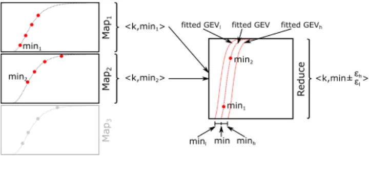
Figure 2 shows an example approximate computation that uses GEV. Each map task computes a part of an optimiza-tion procedure and outputs the minimum value that it finds. (There is only one intermediate key.) The reduce uses the GEV fitting and estimation approach to determine that the desired error bound has been achieved after map tasks 1 and 2 complete. Thus, map task 3 is discarded.
4.
ApproxHadoop
We have implemented the three approximation mecha-nisms [19], along with the error estimation techniques de-scribed in Section 3, in a prototype system called Approx-Hadoop that extends the Approx-Hadoop MapReduce framework. This section describes ApproxHadoop’s interfaces for ap-plication development and job submission, and the changes required to implement the approximation mechanisms and
Map 1 Map 2 Map 3 min <k,min1> <k,min2> <k,min± > minh minl fitted GEV min1 min2 R educe fitted GEVh fitted GEVl min1 min2 εh εl
Figure 2. Example usage of GEV theory in a MapReduce job. Each map task computes the values shown (red points) and reports the minimum. Only maps 1 and 2 are executed. error estimation. As previously mentioned, we limit our dis-cussion to input data sampling and task dropping.
4.1 Developing ApproxHadoop programs
Hadoop offers a set of pre-defined reduce functions (via Java classes) that can be used by programmers (e.g., a re-duce function that sums the values for a given intermediate key). ApproxHadoop similarly offers a set of pre-defined approximation-aware map templates and reduce functions— e.g., classes MultiStageSamplingMapper and Multi
-StageSamplingReducerfor aggregation andApproxMin
-Reducerfor extreme values; see [19] for a complete list.
These classes implement the desired approximation (by leveraging the ApproxHadoop mechanisms), collect the needed information for error estimation (e.g., the total num-ber of data items in a sampled input data block), perform the reduce operation, estimate the final values and the corre-sponding confidence intervals, and output the approximated results. To perform approximations with dropping/sampling, the user inherits ApproxHadoop’s pre-defined classes in-stead of the regular Hadoop classes. The rest of the program remains the same as in regular Hadoop, including the code
formap()andreduce().
Using ApproxHadoop, the word count example from [13] would be adapted as in Figure 3. Only lines #2, #8, and #17 are different than the corresponding Hadoop code.
4.2 Job submission
When the user wants to run an approximate program that uses input data sampling and/or map dropping, she can direct the approximation by specifying either:
1. The percentage of map tasks that can be dropped (drop-ping ratio) and/or the percentage of input data that needs to be sampled (input data sampling ratio); or,
2. The desiredtarget error bound(either as a percentage or an absolute value) at a confidence level.
Users who understand their applications well (e.g., from re-peated execution) can use the first approach. In this case, ApproxHadoop will randomly drop the specified percentage
1 c l a s s ApproxWordCount : 2 c l a s s Mapper e x t e n d s M u l t i S t a g e S a m p l i n g M a p p e r : 3 // k e y : document name 4 // v a l : document c o n t e n t s 5 v o i d map ( S t r i n g key , S t r i n g v a l ) : 6 f o r e a c h word w i n v a l : 7 c o n t e x t . w r i t e (w , 1 ) ; 8 c l a s s R e d u c e r e x t e n d s M u l t i S t a g e S a m p l i n g R e d u c e r : 9 // k e y : a word 10 // v a l s : a l i s t o f c o u n t s 11 v o i d r e d u c e ( S t r i n g key , I t e r a t o r v a l s ) : 12 i n t r e s u l t =0; 13 f o r e a c h v i n v a l s : 14 r e s u l t+=v ; 15 c o n t e x t . w r i t e ( key , r e s u l t ) ; 16 v o i d main ( ) : 17 s e t I n p u t F o r m a t ( A p p r o x T e x t I n p u t F o r m a t ) ; 18 r u n ( ) ;
Figure 3. An example approximate word count MapReduce program using ApproxHadoop.
of map tasks and/or sample each data block with the spec-ified sampling ratio. For supported reduce operations, Ap-proxHadoop will also compute and output error bounds.
In the second case, for the supported reduce operations, ApproxHadoop will determine the appropriate sampling and dropping ratios. For other computations, the user would need to provide code for estimating errors. When the Map phase produces multiple intermediate keys, ApproxHadoop assumes that the specified error bound is the maximum error desired for any intermediate key.
4.3 The ApproxHadoop framework
Input data sampling.We implement input data sampling in new classes for input parsing. These classes parse an input data block and return a random sample of the input data items according to a given sampling ratio. For example,
we implementApproxTextInputFormat, which is similar
to Hadoop’sTextInputFormat. LikeTextInputFormat,
ApproxTextInputFormat parses text files, producing an
input data item per line in the file. Instead of returning all lines in the file, however,ApproxTextInputFormatreturns a sample that is a random subset of appropriate size.
Task dropping.We modified theJobTrackerto: (1) execute map tasks in a random order to properly observe the require-ments of multi-stage sampling, and (2) be able to kill run-ning maps and discard pending ones when they are to be dropped; dropped maps are marked with a new state so that job completion can be detected despite these maps not finish-ing. We also modified the Reducer classes to detect dropped map tasks and continue without waiting for their results.
Error estimation. As already mentioned, our pre-defined approximate Mapper and Reducer classes implement error estimation. Specifically, the Mapper collects the necessary information, such as the number of data items in the input
TaskTrackermT TaskTrackerm9 ReduceTaskm% JobTracker InputmBlockmN MapTaskmN OutputmBlock MultiStage Reducer MultiStage Mapper ApproxInput Format ApproxOutput TaskTrackerm% MapTaskm% MultiStage Mapper x ApproxInput Format Incremental Dropping Mechanism :%. :9. :9. :9. :f. :f. :8. :8. :%C.
lorem sit ipsum nisi ipsum sit laboris nisi ut sit ipsum ut %: 9: f: M%: 666m ipsum ut sit nisi lorem ipsum sit laboris lorem
%: 9: MN:
666m
ipsum ut sit nisi lorem ipsum sit laboris lorem %: 9: MN: 666m ipsum lorem nisi 666m 9f5±9 f57±f 999±% Error Estimator :6. :9. TaskTrackermT TaskTrackerm9 ReduceTaskm% JobTracker InputmBlockmN MapTaskmN OutputmBlock MultiStage Reducer MultiStage Mapper ApproxInput Format ApproxOutput TaskTrackerm% MapTaskm% MultiStage Mapper ApproxInput Format ApproxWordCount map:. reduce:. Targetmerrormbound mm±%3m953mconfidence x Incremental Dropping Mechanism :9. :9. :9. :f. :f. :8. :8. :5. :7. :8. :9. :%C.
lorem sit ipsum nisi ipsum sit laboris nisi ut sit ipsum ut %: 9: f: M%: 666m ipsum ut sit nisi lorem ipsum sit laboris lorem
%: 9: MN:
666m
ipsum ut sit nisi lorem ipsum sit laboris lorem %: 9: MN: 666m ipsum lorem nisi 666m 9f5±9 f57±f 999±% Error Estimator :6. InputmBlockm%
lorem sit ipsum nisi ipsum sit laboris nisi ut sit ipsum ut %: 9: f: M%: 666m InputmBlockm%
lorem sit ipsum nisi ipsum sit laboris nisi ut sit ipsum ut %: 9: f: M%: 666m
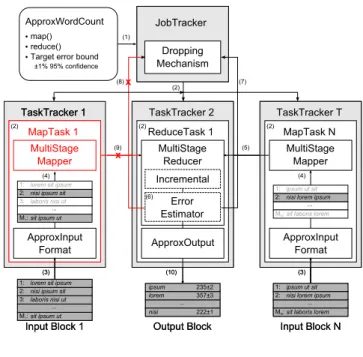
Figure 4. Example execution of the ApproxWordCount program with multi-stage sampling in ApproxHadoop. data block, and forwards it to the Reducer. The Reducer computes the error bounds using the techniques described in Section 3. We have also modified theJobTrackerto collect error estimates from all reduce tasks, so that it can track error bounds across the entire job. This is necessary for choosing appropriate ratios of map dropping and input data sampling.
Incremental reduce tasks. To estimate errors and guide the selection of sampling/dropping ratios at runtime, reduce tasks must be able to process the intermediate outputs be-fore all the map tasks have finished. We accomplish this by adding a barrier-less extension to Hadoop [44] that allows reduce tasks to process data as it becomes available.
Example execution. Figure 4 depicts a possible approxi-mate execution of the ApproxWordCount program. The user first submits the job (arrow 1), specifying a target error bound and confidence level. TheJobTracker then starts N map tasks (only two are shown) and 1 reduce task (2). Each map task executes by sampling its input data block (3 & 4). Map task N finishes first and reports its statistics to the re-duce task (5). The rere-duce task estimates the error bounds (6), decides that the target has been achieved, and so asks the JobTrackerto terminate the remaining map tasks (7). The JobTrackerthen kills map task 1, which may still be exe-cuting (8). The reduce task is informed that map task 1 will not complete (9), allowing it to complete its execution and output the results (10).
4.4 Estimating and bounding errors for aggregation
To compute the error bounds when multi-stage sampling is used, we need to know which cluster (i.e., input data block) each key/value pair came from. Thus, each map task tags
each key/value pair that it produces with its unique task ID. Each map task processing an input data blockialso tracks the number of units (i.e., data items) Mi in the block, as
well as the number of sampled unitsmi. This information
is passed to all of the reduce tasks. We implement this func-tionality in our pre-defined Mapper and Reducer classes.
User-specified dropping/sampling ratios. The computa-tion is straightforward when the user specifies the ratios. The framework randomly chooses the appropriate number of map tasks and executes them. Each task is directed to sample the input data block at the user-specified sampling ratio. The reduce tasks then compute the error bounds as discussed in Section 3.1.
User-specified target error bound.Selecting dropping/sam-pling ratios is more challenging when the user specifies a target error bound, because the ratios required to achieve the bound depend on the variance of the intermediate val-ues. Also, different combinations ofn(number of clusters) andmi/Mi(sampling ratio within each cluster) will achieve
similar error bounds.
Our approach for choosingnandmi is as follows.
Sup-pose that a subsetn1of map tasks are executed first and the
target error is X%. The framework collects information from these tasks to guide the sampling of the remaining map tasks. Specifically, we want to find the minimum amount of time required to complete the job while meeting the constraint:
tn−1,1−α/2
q d
V ar(ˆτ)≤X%×τˆ (4)
Thus, we set up an optimization problem and solve it. The optimization problem is to minimize the remaining execu-tion time RET = n2tmap( ¯M ,m¯), wheren2 is the
num-ber of remaining map tasks, andtmap( ¯M ,m¯)is the time
re-quired to execute a map task withM¯ input data items, pro-cessing onlym¯ items. Note that this assumes that the input data is equally divided among the map tasks, and that pro-cessing time for each data item does not vary greatly. We model the running time of a map task as:
tmap(M, m) =t0+M tr+mtp (5)
wheret0is the base time to start a map andtrandtpare the
average times required to read and process one data item, respectively. We do not model or optimize the running time of reduce tasks, because the Map phase is typically the most time-consuming, and optimizing for the map tasks usually decreases the reduces’ runtime.
We also rewrite Equation 3 as:
d V ar(ˆτ) =N(N−n)s 2 u n + N nCV ar (6) where CV ar=n2M¯( ¯M−m¯) ¯ s2 ¯ m + n1 X i=1 Mi(Mi−mi) s2 i mi (7)
Finally, we estimateto,tr,tp,M¯, and¯susing statistics
gathered from the execution of then1completed map tasks.
We then solve forn2andm¯ using binary search, under the
constraint given by Equation 4,n = n1+n2, andn2 ≤
N−n1. The time required to solve the problem is negligible
(compared to the time to compute the approximate result and its error bounds), even for large numbers and sizes of clusters.
By default, for a job using multi-stage sampling with a user-specified target error bound, ApproxHadoop executes the first wave of map tasks without sampling. It then uses statistics from this first wave to solve the optimization prob-lem and set the dropping/sampling ratios for the next wave. After the second wave, it selects ratios based on the previous two waves, and so on.
The above approach implies that a job with just one wave of map tasks cannot be approximated. However, the user can set parameters to direct ApproxHadoop to run a small number of maps at a specific sampling ratio in a first pilot wave. Statistics from this pilot wave are then used to select dropping/sampling ratios for the next (full) wave of maps. This reduces the amount of precise execution and allows ApproxHadoop to select dropping/sampling ratios even for jobs whose maps would normally complete in just one wave. Running such a pilot wave may lengthen job execution time (e.g., by running two waves of maps instead of one), but can increase system throughput and decrease energy consump-tion because fewer maps are executed without sampling.
4.5 Estimating and bounding errors for extreme values
To compute the error bounds when GEV is used, the Reducer needs to know whether the values it receives for each key are already in Block Minima/Maxima format. If not, the Reducer transforms the data to this format.
User-specified dropping ratio.The framework only runs a randomly chosen subset of maps as specified by the user. The reduce then estimates the min/max and corresponding error bounds, as discussed in Section 3.2.
User-specified target error bound.The reduce estimates the min/max and the error bounds as each map completes. The overhead of this estimation is negligible. When the tar-get error bound has been achieved, the reduce asks the Job-Trackerto kill and/or drop all remaining maps. The reduce will then observe that all maps have completed (or been dropped) and will complete the overall computation.
5.
Evaluation
We evaluate ApproxHadoop using applications with vary-ing characteristics (see Table 1) and usvary-ing various mations for each application. We first explore the approxi-mation mechanisms and errors for some of the applications when users specify the dropping/sampling ratios. Next, we evaluate ApproxHadoop’s ability to dynamically adjust its approximations to achieve user-specified target error bounds
Approx.
Application Input data Size S D U Err.
Page Length Wikipedia dump 9.8GB 3 3 MS Page Rank (40GB) 3 3 MS Request Rate Wikipedia log 3 3 MS Project Popul 46GB 3 3 MS Page Popul (217GB) 3 3 MS Request Rate Webserver log 3 3 MS Page Popul 3 3 MS Page Traffic 3 3 MS Total Size 330MB 3 3 MS Request Size (11GB) 3 3 MS Clients 3 3 MS Client Browser 3 3 MS Attack Freq 3 3 MS
DC Placement US and Europe 480KB 3 3 GEV
Video Encoding Movie 816MB 3 U
K-Means Apache mail list 7.3GB 3 U
Table 1. List of evaluated applications. Approximations: sample input data (S), drop computation (D), and user-defined approximation (U). Error estimation: multi-stage sampling (MS), generalized extreme values (GEV), and user-defined (U).
while minimizing execution time. Finally, we explore Ap-proxHadoop’s sensitivity to the distribution of key values, job sizes (and the impact on energy consumption), and input data sizes.
5.1 Methodology
Hardware. We run our experiments on a cluster of 10 servers (larger experiments on a 60 server cluster). Each server is a 4-core (with 2 hardware threads each) Xeon ma-chine with 8GB of memory and one 164GB 7200rpm SATA disk. The cluster is interconnected with 1Gb Ethernet. Each server consumes 60 Watts when idle and 150 Watts at peak. Reported energy consumption numbers are based on a power model we built from measuring one server. We use a sepa-rate client machine to submit jobs, measuring job execution times on this client.
Software.ApproxHadoop extends Hadoop 1.1.2. Each server
hosts a TaskTracker andDataNode, while one server also
hosts the JobTracker and NameNode. We configure each
server to have 8 map slots and 1 reduce slot. Experiments with multiple reduce tasks always run with the number of reduce tasks equal to the cluster size.
Metrics and measurements.Evaluation metrics include job execution time, energy consumption, and accuracy. For ac-curacy, we report the actual errors between approximate and precise executions, as well as the estimated 95% confidence intervals for the approximate executions. When a job out-puts multiple key-value pairs, we report the actual error and confidence interval for the key with the maximum predicted absolute error. We repeat each experiment 20 times and often report the average, minimum, and maximum for each metric.
104 105 106 107 500 1000 1500 2000 2500 3000 Numbe r of articles
Page size (bytes) (a) Wikipedia Length
Approximate Precise 104 105 106 Numbe r of links
Top 100 linked-to pages (in descending order) (b) Wikipedia Page Rank
100 101 102 103 104 105 106 107 108 109 1010 Numbe r of accesses
Project accesses (in descending order) (c) Wikipedia Project Popularity
Approximate Precise 105 106 107 108 Numbe r of accesses
Top 100 accessed pages (in descending order) (d) Wikipedia Page Popularity
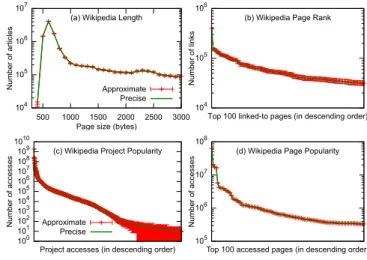
Figure 5. Results of data analysis for (a) WikiLength and (b) WikiPageRank; and log analysis for (c) Project Popular-ity and (d) Page PopularPopular-ity. The error bars show the intervals of one approximated run at 1% input data sampling ratio.
5.2 Results for user-specified dropping/sampling ratios Data Analysis.We study two publicly available large-scale data analysis applications, WikiLength and WikiPageRank, that analyze all English Wikipedia articles. These applica-tions are representative of large-scale processing on collec-tions of Web pages (e.g., for Web search). WikiLength pro-duces a histogram of lengths of the articles [45], with the Map phase producing a key-value pair<s,1>for each arti-cle whose size is in binsand the Reduce phase summing the count for each keys. WikiPageRank counts the number of articles that point to each article [24], emulating one of the main processing components of PageRank [32]. The Map phase of this application produces a pair<a,1>for each link that it finds to articleaand the Reduce phase sums the count for each keya.
We use the Mapper and Reducer classes that implement multi-stage sampling to create approximation-enabled ver-sions of WikiLength and WikiPageRank. We then use the applications to analyze the May 2014 snapshot of Wikipedia [45, 46]. This snapshot contains more than 14 million arti-cles and is compressed into 9.8GB using bzip2 to allow ran-dom access by the map tasks. (Uncompressed, the snapshot requires 40GB of storage.) The 9.8GB partitions into 161 blocks and thus our jobs have 161 maps, running in a little more than two waves in the Xeon cluster.
Figures 5(a) and 5(b) plot parts of the results for a precise execution and an approximate execution with an input data sampling ratio of 1% (each map task processes 1 out of ev-ery 100 input data items) for each application. The error bars show the 95% confidence intervals of the approximated val-ues. Taking one size for WikiLength as an example, consider the values for 1000B articles; the precise value is 230,793,
0 20 40 60 80 100 0.01 0.1 1 10 100 Perce ntage (%)
Input data sampling ratio (%) (a) WikiLength not dropping maps
Precise runtime Approximate runtime Approximation error 95% confidence interval
0.01 0.1 1 10 100
Input data sampling ratio (%) (b) WikiLength dropping 25% maps
0.01 0.1 1 10 100
Input data sampling ratio (%) (c) WikiLength dropping 50% maps
0 50 100 150 200 Runtim e (secon ds)
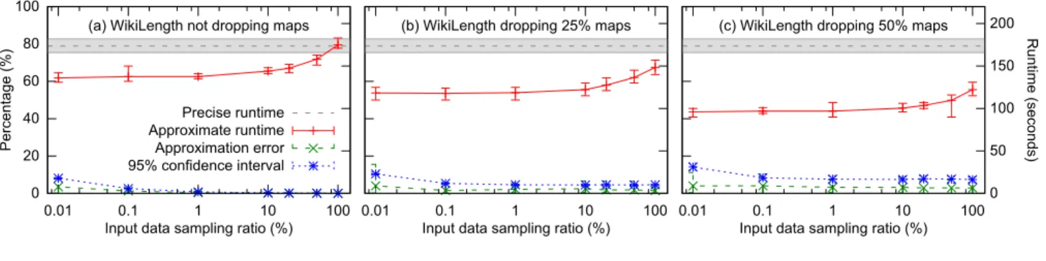
Figure 6. Performance and accuracy of WikiLength for different dropping/sampling ratios.
while the approximated value is 221,802±9,165. The actual error is 8,991 (i.e., 3.89% = (230,793 - 221,802)/230,793).
Figure 6 shows the impact of approximations on the run-time (Y-axis on right) and estimation errors (Y-axis on left) for WikiLength. Each data point along a curve in the graphs plots the average value (over 20 executions) for the corre-sponding metric, and a range bar limited by the minimum and maximum values (over the 20 executions) of the metric. The gray horizontal band across each graph depicts the range of runtimes from multiple runs of the precise program.
Figure 6(a) shows the impact of different input data sam-pling ratios when no map tasks were dropped. Observe that
runtime can be reduced by 21% (173.6 →137.5 secs) by
processing 1% of the articles, resulting in a 95% confidence interval of 0.81% and an actual error of 0.34%. Figures 6(b)-(c) show the impact of combining task dropping with input data sampling. Observe that dropping tasks reduces execu-tion times more than input data sampling, but with wider confidence intervals. For example, by dropping 50% of the maps, we can reduce the runtime to below 105 secs. How-ever, even without input data sampling (i.e., 100% sampling ratio), the confidence interval at this dropping ratio is 7.38% while the actual error is 2.83%.
Task dropping has a stronger impact on execution times because it eliminates all processing (data block I/O accesses and computation on data items) for each dropped block, whereas input data sampling still requires all data items in a block to be read even though some of them will not be processed as part of the chosen sample. On the other hand, task dropping leads to wider confidence intervals for two reasons: (1) data within blocks usually has “locality” (e.g., the data was produced close in time), and (2) sampling within blocks (input data sampling) adds more randomiza-tion than sampling blocks (task dropping), because in our setup, block sizes are substantially larger than the number of
blocks (M N).
Though not shown in the figures, the approximate version of WikiLength does miss sizes for which counts are small (rare occurrences). For example, in the case of 1% input data sampling, counts were reported for 1028 sizes compared to
5018 in the precise computation. For these missing sizes, the error bound was±197, which is substantially smaller than the maximum error bound,±33,480, for the sizes that we did find. This is consistent with our discussion of the limitations of multi-stage sampling in Section 3.1.
To quantify theoverheadof our implementation, we com-pare the runtime of the precise version against the approxi-mation with no sampling and no dropping. In this case, the average runtime increases from 173.6 to 175.0 secs, which is less than 1%.
While not shown here, results for WikiPageRank show the exact same trends (although the overhead is somewhat larger at close to 8%) [19]. Thus, in summary, we observe that input data sampling and map dropping can lead to sig-nificantly different impacts on job runtime and error bounds. Properly combining the two via multi-stage sampling can lead to the lowest runtime for specific error bound targets (and vice versa).
Log Processing.Log processing is a second important type of data analysis commonly done using MapReduce [8]. Thus, we use ApproxHadoop to process the access log for Wikipedia [46]. This log contains log entries for the first week of 2013 and is compressed into 46.0GB (216.9GB uncompressed).
In this case, each unit is an access log entry containing in-formation like access date, access page, and request size. We compute the Project Popularity (the English project, rooted
athttp://en.wikipedia.org, is the most popular project
across more than 2,064 projects with more than 1.9 billion
accesses) and Page Popularity (http://en.wikipedia.
org/wiki/Main_Pageis the most accessed page).
Figures 5(c) and 5(d) plot the results for a precise execu-tion and an approximate execuexecu-tion with an input data sam-pling ratio of 1% for the two programs. Though the con-fidence intervals for unpopular projects may seem large in Figure 5(c), this effect is caused by reporting small num-bers in log scale. These intervals are actually narrower than those for more popular projects. Figure 7 plots the runtime and errors for Project Popularity, as a function of the drop-ping/sampling ratios. The figure shows very similar trends to
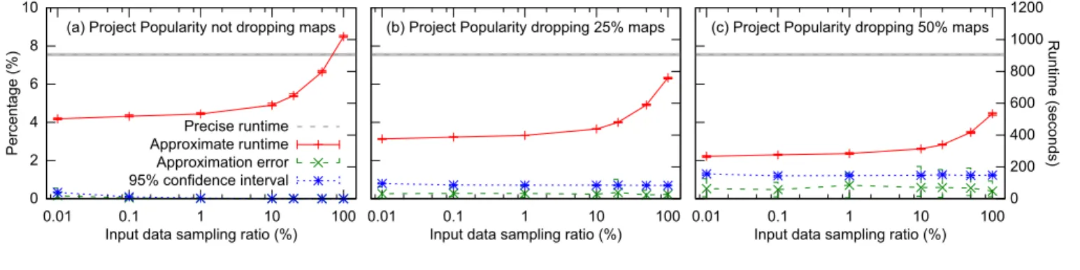
0 2 4 6 8 10 0.01 0.1 1 10 100 Perce ntage (%)
Input data sampling ratio (%) (a) Project Popularity not dropping maps
Precise runtime Approximate runtime Approximation error 95% confidence interval
0.01 0.1 1 10 100
Input data sampling ratio (%) (b) Project Popularity dropping 25% maps
0.01 0.1 1 10 100
Input data sampling ratio (%) (c) Project Popularity dropping 50% maps
0 200 400 600 800 1000 1200 Runtim e (secon ds)
Figure 7. Performance and accuracy of Wikipedia log processing for Project Popularity.
those for WikiLength. The overhead when executing the ap-proximate version without sampling/dropping is 12%. (Note that, when dropping maps, some of the actual errors are larger than the confidence intervals; only 95% of the estima-tions are expected to fall in the 95% confidence intervals).
Datacenter (DC) Placement.We now explore the impact of approximation on an optimization application. Specifically, the application uses simulated annealing to find the lowest costing placement of a set of datacenters in a geographic area (e.g., the US), constrained by a maximum latency to clients (e.g., 50ms) [18]. The area is divided into a two dimensional grid, with each cell in the grid as a potential location for a datacenter. In the MapReduce program, each map executes an independent search through the solution space, outputting the minimum cost placement that it finds. The single reduce task outputs the overall minimum cost placement.
Note that this application itself is already an approxima-tion: the optimization is not guaranteed to produce an opti-mal result, but will produce better results as the search be-comes more comprehensive and/or a finer grid is used. We enhance the capabilities for approximations in this applica-tion by allowing the dropping of map tasks. We use the Map-per and Reducer classes implementing extreme value to es-timate an approximate minimum value and the confidence interval along with the actual minimum cost solution found.
Figure 8 shows the impact of map dropping on the opti-mization with a 50ms maximum latency constraint and the default grid size. We run the experiments with 80 map tasks, with each server configured with only 4 map slots, which is the most efficient setting for this CPU-bound application. Note that the runtime decreases slowly with map dropping (right-to-left) until about 50% of the maps are dropped. This sharp drop in runtime results from the dropping of an en-tire wave of maps. Error bounds also grow relatively slowly until we drop more than 50% of the maps. Targeting error bounds of at most 10%, we drop 70% of the maps to reduce the runtime by 51%.
5.3 Results for user-specified target error bounds
We now demonstrate ApproxHadoop’s ability to achieve a given target error bound by dynamically adjusting the
drop-0 20 40 60 80 100 0 20 40 60 80 100 0 100 200 300 400 500 Perce ntage (%) Runtime (seconds) Executed maps (%) Approximate runtime Approximation error 95% confidence interval
Figure 8. Performance and accuracy of DC Placement for different dropping ratios. The optimization targets a network of datacenters with a 50ms max latency.
ping/sampling ratios. We consider two applications, log pro-cessing and optimization, which use multi-stage sampling and extreme value theory for approximation, respectively.
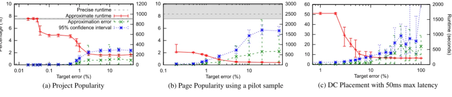
Log Processing. Figure 9(a) plots the runtime and errors as a function of the target error bound for Project Pop-ularity. For small target errors (<0.05%), ApproxHadoop decides that no approximation is possible. Thus, in these cases, there are no errors and the runtimes are the same as for the precise version (the overheads are negligible). From 0.05% to 0.5%, ApproxHadoop is able to use different in-put data sampling ratios to reduce the runtimes by more than 37%. Above 0.5%, ApproxHadoop can start dropping maps to further reduce the runtimes. For example, for a 1% tar-get error, ApproxHadoop reduces the runtime from 908 to 360 secs (60%). Finally, for target errors above 2%, the re-quired error bound is achieved after the 1st wave of map tasks complete, allowing all remaining maps to be dropped. Thus, ApproxHadoop cannot reduce runtime further, giving a maximum runtime reduction of 79%. Importantly, Approx-Hadoop achieved the target error bounds in all experiments, as shown by the 95% confidence interval curve.
Page Popularity presents a more interesting case. The pre-cise version cannot be executed without memory-swapping in our cluster. In fact, our memory capacity is not even large enough to run the first wave of maps precisely without swap-ping. However, it is possible to compute Page Popularity
ef-0 2 4 6 8 10 0.01 0.1 1 10 0 200 400 600 800 1000 1200 Perce ntage (%) Runtime (seconds) Target error (%) Precise runtime Approximate runtime Approximation error 95% confidence interval
(a) Project Popularity
0 2 4 6 8 10 0.1 1 10 0 500 1000 1500 2000 2500 3000 Perce ntage (%) Runtime (seconds) Target error (%)
(b) Page Popularity using a pilot sample
0 10 20 30 40 50 60 1 10 100 0 500 1000 1500 2000 Perce ntage (%) Runtime (seconds) Target error (%)
(c) DC Placement with 50ms max latency
Figure 9. Performance and accuracy for Project Popularity when targeting different maximum errors.
ficiently for this log by directing ApproxHadoop to use a small pilot wave (see end of Section 4.4).
Figure 9(b) plots the behavior of Page Popularity, when ApproxHadoop relies on a pilot sample ran with a1%input data sampling ratio. (The pilot takes an average of93±11
secs to complete for this application.) The results show that we cannot target errors lower than 0.2%. Note that the execu-tion time is somewhat variable at the 0.2% target error, as the reduce tasks memory-swap in some experiments. For larger target bounds, ApproxHadoop can approximate enough that swapping does not occur. Overall, the use of the pilot sample improves performance significantly. For example, assuming a target bound of 1%, the pilot sample reduces the execution time by 78% compared to the precise execution, and 80% compared to ApproxHadoop without the pilot sample. (We include the time to perform the pilot in these calculations.) Finally, note again that all confidence intervals are smaller than the target error bounds.
DC Placement.Figure 9(c) plots the runtime and errors, as a function of the target error bounds, for an execution with 320 map tasks. Since this application uses only task dropping and the errors introduced by dropping maps are relatively large, ApproxHadoop cannot improve execution time until the tar-get bound is larger than 2%. (Note that we are showing errors for these cases, even though ApproxHadoop is not perform-ing any approximation, because the application itself is an approximation.) At6%, ApproxHadoop reduces the runtime by more than 80% by dropping 285 maps. For targets higher than 6%, ApproxHadoop achieves the target error after pro-cessing the first wave of maps, and so it drops all remain-ing maps. Thus, ApproxHadoop can reduce runtime by up to 87%, while consistently achieving the target bound.
5.4 Sensitivity analysis
Impact of the distribution of key values.An important fac-tor when estimating errors is the distribution of the program outputs (key values). We now evaluate the impact of this dis-tribution by considering Log Processing on a log with differ-ent characteristics, our departmdiffer-ent’s Web server access log. The log spans 80 weeks from November 2012 to June 2014 and contains more than 40 million requests. The compressed size of the log is 330MB, while the original size is 11GB.
The data is divided into 80 files (one per week), each of which fits in a single data block (i.e.,<64MB). Each unit in the files is an access (a line), which contains information like timestamp, accessed page, and page size.
We study two applications that analyze: (1)Request Rate: computes the average number of requests per time unit (e.g., each hour within a week), and (2)Attack Frequencies: com-putes the number of attacks (for a set of well-known attack patterns) on the Web server per client.
Figure 10(a) plots a precise and an approximate execution of Request Rate with an input data sampling ratio of 1%. The figure shows the pattern of request rates that one would expect for a Web site, as well as small errors and narrow confidence intervals. For the same execution, Figure 10(b) plots the request rates in descending order. This figure shows that request rates are fairly stable (they vary by roughly 33%), i.e. quite a different distribution than what we see in Figure 5. Despite this significantly different distribution, Figure 11(a) shows that the impact of varying the input data sampling ratio is very similar to Figures 6 and 7.
More interestingly, consider the precise and approximate results for Attack Frequencies in Figure 10(c), again with 1% input data sampling ratio. Since this application com-putes rare values, we see larger errors and wider confidence intervals. Figure 11(b) shows that ApproxHadoop can re-duce execution time significantly at the cost of higher errors and wider intervals. This application emphasizes the fact that approximation is most effective for estimating values com-puted from a large number of input data items, rather than those from only a few.
Impact of job size on energy consumption. One of the goals of approximate computing is to conserve energy. By reducing the execution time, as in the experiments so far, and not increasing the power consumption, we save energy. The energy savings is roughly proportional to the reduction in execution time. However, in certain scenarios, Approx-Hadoop can also save energy independently of reductions in execution time.
To see this, consider the experiments processing our de-partment’s Web server log. They show that input data sam-pling reduces the runtime (Figure 11), but dropping maps has
Num ber of accesses ( in thousand s) 200 250 300 350
Hourly request rates (in descending order) (b) Request Rate 0 50 100 150 200 Num ber of attacks
Attacker attacks (in descending order) (c) Attack Frequencies Approximate Precise Num ber of accesses ( in thousand s) 200 250 300 350
Mon Tue Wed Thu Fri Sat Sun
(a) Request Rate
Figure 10. Results of processing our Web server log.
0 20 40 60 80 100 0.01 0.1 1 10 100 0 10 20 30 40 50 Perce ntage (%) Runtime (seconds)
Input data sampling ratio (%) (a) Request Rate
Precise runtime Approximate runtime Approximation error 95% conf interval 0 20 40 60 80 100 0.01 0.1 1 10 100 0 10 20 30 40 50 Perce ntage (%) Runtime (seconds)
Input data sampling ratio (%) (b) Attack Frequencies
Figure 11. Performance and accuracy of Web server log processing: (a) Request Rate and (b) Attack Frequencies.
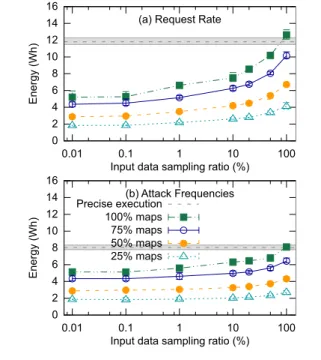
no significant effect when jobs have a single wave of maps. (Recall that when the user specifies the dropping/sampling rates, they can be applied in the first wave of maps.) The same may occur for applications that have a few more waves as well. For applications where dropping maps does not re-duce the runtime, we can transition the servers that have no maps to execute (corresponding to the maps that were dropped) to a low-power state (i.e., ACPI S3) when they be-come idle. Figure 12 shows the energy consumptions result-ing from both droppresult-ing maps and input data samplresult-ing for Request Rate and Attack Frequencies. As we would expect, decreasing the amount of input data ApproxHadoop sam-ples reduces energy consumption, as this reduces execution time. However, dropping more maps also saves energy, even though this does not reduce execution time.
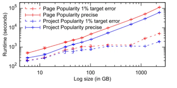
Impact of data size.Finally, we evaluate the impact of the dataset size on ApproxHadoop by running Log Processing on a larger Wikipedia access log. The log has one file per day of the year for a total of 365 files and 12.5TB, which become 2.3TB when compressed. We experiment with dif-ferent subsets of the log, as we list in Table 2. Our Log Pro-cessing experiments on Wikipedia so far have only used the first week’s data.
Because our Xeon cluster does not have enough disk space, for these experiments, we use another cluster with 60 nodes and a total disk capacity of 14TB. Each server in this cluster is a 2-core (with 2 hardware threads each) Atom machine with 4GB of memory, one 250GB 7200rpm SATA disk (200GB for data), interconnected with 1Gb Ethernet.
0 2 4 6 8 10 12 14 16 0.01 0.1 1 10 100 Ener gy (Wh)
Input data sampling ratio (%) (a) Request Rate
0 2 4 6 8 10 12 14 16 0.01 0.1 1 10 100 Ener gy (Wh)
Input data sampling ratio (%) (b) Attack Frequencies Precise execution 100% maps 75% maps 50% maps 25% maps
Figure 12. Energy in processing our Web server log using (a) Request Rate and (d) Attack Frequencies for multiple dropping/sampling ratios.
We configure each Atom server with 4 map slots and 1 reduce slot.
Figure 13 compares the runtime of the precise and ap-proximate (targeting a 1% maximum error with 95% con-fidence) executions of Project and Page Popularity. As one would expect for these applications, the figure shows that the runtime of the precise program scales linearly with the in-put size. More importantly, approximating the results short-ens runtimes significantly, especially for the larger input sizes.For example, the approximate executions of Project and Page Popularity for the year are more than32×and20× faster, respectively, while always achieving error bounds lower than 1%.
6.
Related work
Researchers have explored numerous approximation tech-niques at the language [6, 38] and hardware [39] levels, for query processing [4, 10, 42], and for distributed
sys-Period Accesses Compress Uncompress #Maps 1 day 499M 5.7 GB 27.0 GB 92 2 days 1.1G 12.4 GB 58.7 GB 201 5 days 2.8G 32.1 GB 151.7 GB 518 1 week 4.0G 46.0 GB 216.9 GB 740 10 days 5.9G 67.5 GB 317.9 GB 1086 15 days 9.0G 103.2 GB 484.9 GB 1661 1 month 19.4G 221.8 GB 1.0 TB 3567 3 months 55.8G 633.1 GB 2.9 TB 10172 6 months 109.2G 1.2 TB 5.7 TB 19947 1 year 234.2G 2.3 TB 12.5 TB 38246
Table 2. Sizes of the Wikipedia access log [46] for different periods starting on January 1st 2013.
102 103 104 105 10 100 1000 Runtime (seconds)
Log size (in GB) Page Popularity 1% target error Page Popularity precise Project Popularity 1% target error Project Popularity precise
Figure 13. Performance of Page and Project Popularity for different log sizes. Both axes are in log scale.
tems [12, 21, 33]. They have also explored techniques for probabilistic reasoning about approximate programs [7, 9, 23, 28, 34, 40, 47]. We discuss the most closely related works on approximation in this section.
Approximation mechanisms.Slauson and Wan [43] have studied map task dropping in Hadoop. Riondatoet al.[36] have used input data sampling with error estimation in a spe-cific MapReduce application. However, these works have not considered the two mechanisms together, nor did they consider a general framework for error estimation in the presence of both mechanisms. Rinard [35] has also studied task dropping, albeit in an entirely different approach that requires previous executions with known output and signifi-cant pre-computation for estimating errors.
Our proposed sampling/dropping mechanisms are also related to loop/code perforation techniques in SpeedPress for sequential code [22, 29–31, 41]. Green [6] similarly provides a framework to adapt the approximation level based on the defined quality of service for sequential code. Bornholtet al. [9] propose uncertain data types to abstract approximations at the language level (e.g., C#) and estimate errors from approximate data sources (e.g., GPS). Unlike these systems for sequential code, ApproxHadoop proposes mechanisms for distributed MapReduce programs.
Paraprox [37] creates approximate data-parallel kernels using function memoization and runtime tuning. The execu-tion is checked a posteriori using an easily checkable quality
metric. In contrast, ApproxHadoop provides statistical error bounds around the computed approximate results within a distributed MapReduce framework.
Approximations in query processing. In the domain of database query processing, Garofalakiset al.[17] use wavelet-coefficient synopses and Chaudhuri et al. [10] use strati-fied sampling to build samples to provide bounded errors. SciBorq [42] also builds samples based on past query re-sults. BlinkDB [4] uses stratified sampling to produce data samples with the desired characteristics before the execu-tion of the queries. In contrast, we focus on the MapReduce paradigm, and use multi-stage sampling (stratified sampling is a subset) to compute approximations online without pre-computation. Online sampling is a powerful tool for MapRe-duce environments, where large data sets (e.g., logs) are of-ten processed only a few times (or even just once).
MapReduce and Hadoop.MapReduce Online [12] mod-ifies Hadoop to avoid the barrier between the Map and Reduce phases, and outputs intermediate (called “approx-imate”) results during the execution of the reduce tasks. However, unlike ApproxHadoop, it does not attempt to com-pute error bounds. GRASS [5] uses speculation to reduce the impact of straggler tasks in jobs that need not complete all their tasks. In contrast, ApproxHadoop drops remaining map tasks when a target error bound has been achieved or a target percentage of map tasks has been completed.
7.
Conclusions
In this paper, we proposed a general set of mechanisms for approximation in MapReduce, and demonstrated how to use existing statistical theories to compute error bounds (95% confidence intervals) for popular classes of approxi-mate MapReduce programs. We also implemented and eval-uated ApproxHadoop, an extension of the Hadoop data-processing framework that supports our rigorous approxi-mations. Using extensive experimentation with real systems and applications, we show that ApproxHadoop is widely ap-plicable, and that it can significantly reduce execution time and/or energy consumption when users can tolerate small amounts of inaccuracy. Based on our experience and re-sults, we conclude that our framework and system can make efficient and controlled approximation easily accessible to MapReduce programmers.
Acknowledgments
We thank A. Verma and his co-authors for the barrier-less extension to Hadoop [44]. We also thank David Carrera and the reviewers for comments that helped us improve this paper. This work was partially supported by NSF grant CSR-1117368 and the Rutgers Green Computing Initiative.
References
[2] Apache Mahout.http://mahout.apache.org.
[3] Apache Nutch.http://nutch.apache.org.
[4] S. Agarwal, B. Mozafari, A. Panda, H. Milner, S. Madden, and I. Stoica. BlinkDB: Queries with Bounded Errors and Bounded Response Times on Very Large Data. InProceedings
of the European Conference on Computer Systems (EuroSys),
2013.
[5] G. Ananthanarayanan, M. Hung, X. Ren, I. Stoica, A. Wier-man, and M. Yu. GRASS: Trimming Stragglers in Approxi-mation Analytics. InProceedings of the USENIX Symposium
on Networked Systems Design and Implementation (NSDI),
2014.
[6] W. Baek and T. M. Chilimbi. Green: A Framework for
Supporting Energy-Conscious Programming using Controlled
Approximation. InProceedings of the ACM SIGPLAN
Con-ference on Programming Language Design and
Implementa-tion (PLDI), 2010.
[7] S. Bhat, J. Borgstr¨om, A. D. Gordon, and C. Russo. Deriving Probability Density Functions from Probabilistic Functional Programs. InProceedings of the International Conference on Tools and Algorithms for the Construction and Analysis
of Systems (TACAS), 2013.
[8] S. Blanas, J. M. Patel, V. Ercegovac, J. Rao, E. J. Shekita, and Y. Tian. A Comparison of Join Algorithms for Log Processing in MapReduce. InProceedings of the ACM SIGMOD
Interna-tional Conference on Management of Data (SIGMOD), 2010.
[9] J. Bornholt, T. Mytkowicz, and K. S. McKinley.
Uncertain<T>: A First-Order Type for Uncertain Data.
InProceedings of the International Conference on
Architec-tural Support for Programming Languages and Operating
Systems (ASPLOS), 2014.
[10] S. Chaudhuri, G. Das, and V. Narasayya. Optimized Stratified Sampling for Approximate Query Processing.ACM
Transac-tions on Database Systems (TODS), 32(2), 2007.
[11] S. Coles. An Introduction to Statistical Modeling of Extreme
Values. Springer, 2001.
[12] T. Condie, N. Conway, P. Alvaro, J. M. Hellerstein, K. Elmele-egy, and R. Sears. MapReduce Online. InProceedings of the USENIX Symposium on Networked Systems Design and
Im-plementation (NSDI), 2010.
[13] J. Dean and S. Ghemawat. MapReduce: Simplified Data Pro-cessing on Large Clusters. InProceedings of the Symposium
on Operating Systems Design and Implementation (OSDI),
2004.
[14] A. Doucet, S. Godsill, and C. Andrieu. On Sequential Monte Carlo Sampling Methods for Bayesian Filtering.Statistics and
Computing, 10(3), 2000.
[15] J. Ekanayake, S. Pallickara, and G. Fox. MapReduce for Data Intensive Scientific Analyses. InProceedings of the IEEE
International Conference on e-Science (e-Science), 2008.
[16] Z. Fadika, E. Dede, M. Govindaraju, and L. Ramakrishnan. Adapting MapReduce for HPC environments. InProceedings of the International ACM Symposium on High-Performance
Parallel and Distributed Computing (HPDC), 2011.
[17] M. N. Garofalakis and P. B. Gibbons. Approximate Query Processing: Taming the TeraBytes. In Proceedings of the
International Conference on Very Large Databases (VLDB),
2001.
[18] I. Goiri, K. Le, J. Guitart, J. Torres, and R. Bianchini. In-telligent Placement of Datacenters for Internet Services. In Proceedings of the International Conference on Distributed
Computing Systems (ICDCS), 2011.
[19] I. Goiri, R. Bianchini, S. Nagarakatte, and T. D. Nguyen. ApproxHadoop: Bringing Approximations to MapReduce Frameworks. Technical Report DCS-TR-709, Department of Computer Science, Rutgers University, 2014.
[20] P. J. Haas, J. F. Naughton, S. Seshadri, and L. Stokes. Sampling-Based Estimation of the Number of Distinct Values of an Attribute. InProceedings of the International
Confer-ence on Very Large Databases (VLDB), 1995.
[21] J. M. Hellerstein, P. J. Haas, and H. J. Wang. Online Aggre-gation. InProceedings of the ACM SIGMOD International
Conference on Management of Data (SIGMOD), 1997.
[22] H. Hoffmann, S. Sidiroglou, M. Carbin, S. Misailovic, A. Agarwal, and M. Rinard. Dynamic Knobs for Respon-sive Power-Aware Computing. InProceedings of the Interna-tional Conference on Architectural Support for Programming
Languages and Operating Systems (ASPLOS), 2011.
[23] O. Kiselyov and C.-C. Shan. Embedded Probabilistic Pro-gramming. InProceedings of the IFIP TC 2 Working
Confer-ence on Domain-Specific Languages (DSL), 2009.
[24] J. Lin. Cloud9: A Hadoop Toolkit for Working with Big Data. http://lintool.github.io/Cloud9.
[25] J. W. Liu, W.-K. Shih, K.-J. Lin, R. Bettati, and J.-Y. Chung. Imprecise Computations. Proceedings of the IEEE, 82(1), 1994.
[26] S. Liu and W. Q. Meeker. Statistical Methods for Estimating the Minimum Thickness Along a Pipeline. Technometrics, 2014.
[27] S. Lohr.Sampling: Design and Analysis. Cengage Learning, 2009.
[28] T. Minka, J. Winn, J. Guiver, S. Webster, Y. Zaykov, B. Yan-gel, A. Spengler, and J. Bronskill. Infer.NET 2.6.
Mi-crosoft Research Cambridge, 2014. http://research.
microsoft.com/infernet.
[29] S. Misailovic, S. Sidiroglou, H. Hoffmann, and M. Rinard. Quality of Service Profiling. InProceedings of the ACM/IEEE
International Conference on Software Engineering (ICSE),
2010.
[30] S. Misailovic, D. M. Roy, and M. C. Rinard. Probabilistically Accurate Program Transformations. In Proceedings of the
International Static Analysis Symposium (SAS), 2011.
[31] S. Misailovic, S. Sidiroglou, H. Hoffmann, M. Carbin,
A. Agarwal, and M. Rinard. Code Perforation:
Automat-ically and DynamAutomat-ically Trading Accuracy for Performance
and Power, 2014. http://groups.csail.mit.edu/cag/
codeperf/.
[32] L. Page, S. Brin, R. Motwani, and T. Winograd. The PageR-ank Citation RPageR-anking: Bringing Order to the Web. Technical