Transfer Learning for High Resolution Aerial Image Classification

Rochester Institute of Technology

RIT Scholar Works

Presentations and other scholarship

Faculty & Staff Scholarship

9-30-2016

Transfer Learning for High Resolution Aerial Image

Classification

Yilong Liang

Sildomar T. Monteiro

Eli S. Saber

Follow this and additional works at:

https://scholarworks.rit.edu/other

This Conference Paper is brought to you for free and open access by the Faculty & Staff Scholarship at RIT Scholar Works. It has been accepted for inclusion in Presentations and other scholarship by an authorized administrator of RIT Scholar Works. For more information, please contact [email protected].

Recommended Citation

Y. Liang, S.T. Monteiro, E.S. Saber "Transfer Learning for High Resolution Aerial Image Classification," IEEE Applied Imagery Pattern Recognition (AIPR) Workshop 2016, Washington, DC, October 2016. arXiv:1510.00098v2

Transfer Learning for High Resolution Aerial Image

Classification

Yilong Liang

, Sildomar T. Monteiro

, Eli S. Saber

∗_{Chester F. Carlson Center for Imaging Science} †_{Department of Electrical and Microelectronic Engineering}

Rochester Institute of Technology, Rochester, NY, 14623 Email:{yxl7245, sildomar.monteiro, esseee}@rit.edu

Abstract—With rapid developments in satellite and sensor technologies, increasing amount of high spatial resolution aerial images have become available. Classification of these images are important for many remote sensing image understanding tasks, such as image retrieval and object detection. Meanwhile, image classification in the computer vision field is revolutionized with recent popularity of the convolutional neural networks (CNN), based on which the state-of-the-art classification results are achieved. Therefore, the idea of applying the CNN for high resolution aerial image classification is straightforward. However, it is not trivial mainly because the amount of labeled images in remote sensing for training a deep neural network is limited. As a result, transfer learning techniques were adopted for this problem, where the CNN used for the classification problem is pre-trained on a larger dataset beforehand. In this paper, we propose a specific fine-tuning strategy that results in better CNN models for aerial image classification. Extensive experiments were carried out using the proposed approach with different CNN architectures. Our proposed method shows competitive results compared to the existing approaches, indicating the superiority of the proposed fine-tuning algorithm.

I. INTRODUCTION

Recently, the remote sensing images have been obtained with increasing spatial and spectral resolutions. The expansion of the spectral domain advances the spectral-related appli-cations, such as material identification. Meanwhile, the the increase in spatial resolution makes the spatial details and tex-tures of the scenes more discernible. Recently, the WorldView-3 satellite sensor provides the images with panchromatic resolution of 0.31m, under which the territorial structures of the scene are accurately captured in the image. Classification of high spatial resolution remote sensing images refers to as-signing semantic labels to recognize the images. The problem has become an ongoing research topic in the past decades due to the the significant role it plays in facilitating many applications such as vegetation monitoring in agriculture, airport security and aviation safety operation in surveillance, land cover change detection in environmental monitoring, and so on.

Within the literature, a large amount of research efforts have been devoted to the image classification problem, fo-cusing on the design of better feature representations of the images. These image representations ranges from low-level ones, such as color autocorrelogram (ACC) [1] and local color histogram (LCH) [2], to mid-level variants, such as bag

of visual words (BoW), and to high-level features that are automatically learned from the image dataset [3]. Recently, deep learning techniques, especially the convolutional neural networks (CNNs), have been applied for image classification in computer vision areas and astounding classification results were achieved. One of the major advantages of applying the CNN approach in computer vision applications is that a large dataset containing millions of labeled images is available for training a robust deep CNN architecture. However, much fewer labeled high resolution aerial images are available. As a result, different transfer learning techniques were adopted in order to apply the CNN approach to classify these images. Transfer learning refers to the technique that pre-trains a deep CNN model on a large but different dataset and then adapts the trained model to specific problems where much smaller image datasets are available.

In this paper, we explore the transfer learning techniques for recognizing the high resolution aerial imagery. First, we extract image features using different pre-trained CNN archi-tectures trained using the ImageNet challenge dataset [4] and learn new classifiers for recognizing our images. Next, we fine-tune the pre-trained CNNs to make the neural network better adapt the aerial imagery. The proposed method was demonstrated to classify the images from the land use land cover (LULC) image dataset [5]. Our contributions include: (1) extract different features using various state-of-the-art CNN architectures for aerial image classification, (2) propose a better fine-tuning framework for remote sensing aerial imagery with small datasets, and (3) perform a comparative study on different transfer learning techniques to better understand the CNN based image features.

II. RELATEDWORK

Image classification has been thoroughly studied in the computer vision field and many algorithms have been pro-posed to solve this problem. Compared to computer vision applications, classification of the aerial images are more chal-lenging given different appearances of the objects randomly rotated within the scene and increasing complexities of the background textures. Initially, the problem was addressed with the bag of word (BoW) model, which extracts image features using the histograms of visual words derived from low level features in the images [5]. However, the BoW model does

not take the spatial relations between these visual words into account and some research efforts have be devoted towards including the spatial context information into the existing model. For example, authors in [5] proposed two algorithms for this purpose: (1) Adopt the spatial pyramid matching kernel (SPMK) introduced by Lazebinik et al. [6] to construct a three-layer pyramid of the image. The image is then represented as a vector concatenated from the BoW representations of these pyramids. (2) Incorporate the co-occurrence kernel (SCK) with the BoW model to compensate for the spatial information. However, as pointed out by Chen et. al. [7], the SCK-BoW is computational infeasible if the number of the visual words is large. Therefore, the author proposed the pyramid of spatial relaton (PSR) model to capture both absolute and relative spatial relationships between local features.

The major disadvantage of the algorithms based on BoW model is that hand-craft low level features, such as SIFT, are required to generate the discriminate descriptors. In order to address this problem, many supervised and unsupervised learning methods have been studied to derive image features from the datasets. On one hand, unsupervised feature learning methods are proposed to learn feature extractors from the image scenes [8], [9]. On the other hand, tremendous pro-gresses have been made on supervised feature learning owing to the development of convolutional neural networks. The groundbreaking work of AlexNet proposed by Krizhevsky et al. [10] learns the image features with a eight-level deep neural network, which consists of five convolution layers and three fully connected layers, using ImageNet [11] consisting of 1000 image categories. The success of the AlexNet lies in several tricks introduced during training, including the application of rectified linear layer, the addition of the “dropout” layer, and the deployment of multiple GPUs. Ever since then, there is an ongoing interest to learn deep CNN architectures for image recognition. Better performances were achieved using other CNN architectures, such as VGG [12], GoogleNet [13], and ResNet [14]. Results from these CNN based algorithms indicate that the more layers the neural network contains, the better results it obtains. However, issues regarding to designing these deep neural network arise as well, leading to many simplification methods of filters to make sure the CNN architectures work properly.

In order to adapt the CNNs for the aerial image classifica-tion, one possible approach is to apply the pre-trained CNN models from the large image dataset, such as ImageNet, to extract features. The first attempt to apply the pre-trained CNN architectures on classifying high resolution aerial images was demonstrated in [3], where the pre-trained neural networks of AlexNet and Overfeat [15] were adopted as feature extractors, and the activation maps form the second last layers of the CNN models were used for image representations. Later on, Castelluccio et. al. [16] proposed to fine-tune the weights of the convolution layers of the pre-trained CNNs to achieve better image features. In order to make use of the outputs from mid-level layers of the CNN, Hu et. al. [17] proposed features that aggregate the outputs from mid-level layers and

last fully connected layers of the CNN structure with feature coding algorithms, showing improvement on the classification results.

III. METHODS

A. Convolutional Neural Networks

The convolutional neural networks (CNNs) provide end-to-end solutions for many image related tasks, such as image segmentation, recognition, and object detection. Usually, the architecture of a CNN model refers to the structure that contains a sequence of different layers concatenated one next to the other. Each layer is characterized with neurons that perform different differentiable mathematical operations, so as to make the neurons learn-able through back-propagation. In general, typical layers include the convolutional (CONV) layer, the pooling (POOL) layer, the rectified linear layer (ReLU), the fully connected (FC) layer, and the softmax (SOFTMAX) layer. The CONV layer contains a bank of three dimensional filters that convolve over the whole input data and outputs a data cube that concatenates different filter outputs together. The POOL layer aims at reducing the spatial size of input feature map with different down-sampling techniques, such as averaging and taking the maximum of local regions of the input. In the FC layer, each neuron is connected to all the output neurons of the previous layer. Therefore, it can be recognized as a special case of convolutional layer whose receptive field covers the entire spatial region of its input. Finally, the SOFTMAX layer is connected to the last FC layer to generate the classification score. In practise, the deep CNN contains many layers and, therefore, the number of learning parameters grows significantly, which leads to the possibility of long training time and data over-fitting. As a result, multiple approaches were proposed to mitigate these problems. For example, the drop out layer (DROP) is used to randomly drop a pre-defined portion of the parameters in the filters and the batch normalization (NORM) is introduced to normalize each channel of the feature map by averaging over spatial locations with a number of instances.

B. Existing CNN architectures for image classification

Based on various combinations of CNN layers with different parameters, a variety of CNN architectures were derived. In this section, four CNN architectures are briefly discussed: AlexNet [10], VGG-F [12], GoogleNet [13], and ResNet [14]. These pre-trained CNN architectures were trained on the ImageNet [11] dataset that contains over hundreds of thousands of images with 1000 classes.

The input image sizes required for AlexNet and VGG-F are

227×227×3 and224×224×3 respectively. The number of filters and their corresponding spatial receptive field are illustrated in Fig. 1. For example, the CONV1 layer in AlexNet contains 96 convolutional filters with receptive filed of11×11, indicating that each filter is convolved with 11×11 spatial regions across the input image. The pooling layers are inserted after the layers of CONV1, CONV2 and CONV5 to reduce the spatial dimensions of the output.

Fig. 1: CNN architectures for AlexNet and VGG-F with the filter specification indicated as: “numer of filters×horizontal receptive field size×vertical receptive field size”

Fig. 2: CNN architecture of GoogleNet (top), where 9 incep-tion modules [13] (bottom) are included.

Being the groundbreaking work for image classification, AlexNet contains five CONV layers and three FC layers. After the pooling operation, the spatial dimension of the CONV5 output becomes 6×6 and thus the spatial receptive field of the FC6 layer is configured as 6×6. Finally, two more FC layers (FC7 and FC8) are concatenated afterwards to generate the classification result. In order to reduce the number of parameters in the AlexNet, the architecture of VGG-F is proposed. The architecture is very similar to that of the AlexNet, except that the number of convolution filters is significantly reduced (from 96 to 64, and 384 to 256) for three CONV layers (CONV1, CONV3, CONV4).

A straightforward way to improve the performance of the neural network is to increase the depth and width of the neural network. However, the complexity of the network increased tremendously as the number of parameters grows aggressively. As a result, the GoogleNet is proposed to address this challenge. The intuition behind the architecture is based on the observation that the correlation within the image pixels tend to be local. Therefore, it is possible to take the local correlations into account to reduce the number of learning parameters. The GoogleNet solves this issue by introducing the inception modules when designing the CNN architecture, as shown in Fig. 2. Each inception module includes a pooling layer and three convolution filters with spatial sizes of1×1,

3×3, and 5×5, in order to cover larger receptive field of each cluster. Responses from these filters are then concatenated together as the module output. The 1×1 convolution layers

Fig. 3: Residual learning block (left) and “bottleneck” building block (right) of ResNet [14]

before the3×3and5×5convolutions are utilized to reduce the dimensions the corresponding filter output. The pooling operation is also utilized since it has shown good performance in previous neural networks, such as AlexNet and VGG-F. It is worth mentioning that the spatial size of these filters are small, being either 1×1,3×3, or 5×5, resulting in significantly reduced number of learning parameters.

The last pre-trained CNN considered in our paper is ResNet [14], which proposed to add residual learning blocks to learn the residual of non-linear function instead of the function itself. The neural network consists of stacks of residual learn-ing blocks, illustrated in Fig. 3. The basic residual learnlearn-ing block simply contains two 3 ×3 CONV layers and learns the difference F(x) between the output F(x) +xand input

x of the block. The “bottleneck” version of the residual learning block is also introduced to reduce the computational complexity through interpolation of1×1convolution layers. The two 1 ×1 CONV layers are inserted to reduce and increase the dimensions of the data, which is very helpful for designing deeper ResNet. Due to the simplicity that each learning block is composed of mostly 3×3 CONV layers, the architecture of ResNet usually becomes very deep. For example, the ResNet-152 [14] stacks multiple “bottleneck” building blocks to generate the deep learning architecture with 152 layers.

C. Proposed Transfer Learning Schemes for Aerial Image Classification

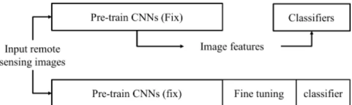
In our paper, two transfer learning schemes are proposed for aerial image classification, as shown in Fig. 4. The first method feeds the image to the pre-trained CNN models and extract image features using the outputs from different layers. Classification algorithms, such as support vector machines or simple linear classifier, are then employed to classify these features. The second method modifies the classification layer of the existing architectures and train the filter weights of the neural network. The parameters of the filters in different layers are initialized from the pre-trained CNN, except for the last classification layer, whose parameters are initialized with random numbers from Gaussian distribution. During fine-tuning, we proposed to train the filter weights of last few layers only and fix the parameters of the filters from other layers. The reasons behind this learning adaptation are twofold. First,

Fig. 4: Proposed transfer learning schemes: extract features from pre-trained CNN architectures (top) and fine-tuning high-level layers in CNN architectures(bottom)

the dataset applied for the transfer learning is relatively small compared to the ImageNet, where the pre-trained models were being trained. Therefore, fine-tuning the whole neural network might not be a good option given the small dataset with limited data. Second, the shallow part of the CNN architectures tend to learn filters that correspond to more general image features, such as edges and corners, which are recognized as fixed features for images from different application fields.

IV. EXPERIMENTALRESULTS

In this section, we validate the proposed algorithm with experiments on high resolution aerial images from the UCMerced Land Use Land Cover (LULC) [5] dataset, where images of 21 categories are present and each category consists of 100 images instances with spatial resolution of 30cm. We adopt five-fold cross validation through our experiment and the dataset is divided into 5 non-overlapping subsets. During the experiment on each fold, images from 4 subsets are utilized for either training a linear classifier with a FC layer or fine-tuning the pre-trained CNNs, and the rest subset is used for testing purpose and generating results. At last, we aggregate the testing results from all the folds by simple averaging operation. Note that we perform data augmentation on the training dataset in both fine-tuning and feature extraction processes. Specifically, the data augmentation procedure crops out a sub-image with required dimensions from the original image and randomly flips the image horizontally.

A. Aerial image classification using pre-trained CNN

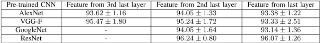
In the first experiment, we extract image features from different layers of the pre-trained CNN architectures. The image features considered are outputs of the FC6, FC7, and FC8 layers for both AlexNet and VGG-F. For GoogleNet and ResNet, we utilize the outputs of the last FC layer and the layer before that as image features. It is worth to mention that out-puts from other layers were not considered since the number of dimensions of the features extracted from them is too large for the limited augmented training dataset in our experiment. For example, the dimensions of the extracted features from the 3rd last layer of GoogleNet and ResNet are 50176 and

100352, which is too large for training a classifier directly given the limited training data. Even though the outputs from the last FC layer (before softmax) of the pre-trained CNNs represent the classification results, we also employ them as image features, which are 1000-dimension vectors. After the

features are extracted, a simple linear classifier is trained by attaching a FC layer to the pre-trained CNN architecture, The weights of the new FC layer are generated from the random Gaussian distribution with a certain variance. At last, the mean and standard deviation of the accuracies across different folds were reported. These statistics, shown in Table I, indicate that the pre-trained CNN models are able to provide image features that generalize well for the aerial images. It is concluded that, for each pre-trained CNN model, the best classification result is obtained with the feature extracted from the 2nd last layer, which is same as classification of the ImageNet dataset. Observations also indicate the possibility of extracting image features using last FC layers, as the classification accuracies from these features are above93%. In addition, we also see that the deeper structure the network becomes, the better performance the classification performance is achieved. Comparisons from the four pre-trained CNNs show that the best performance is obtained when the ResNet-152 is used as the feature extractor, with the average accuracy of 96.24%. Even with the features from the last FC layer, the accuracy achieved is96.07%, which is superior to any of features from other pre-trained CNNs.

B. Aerial image classification using fine-tuned CNN

From the first experiment, we observed that the features from the last few layers of pre-trained CNN architectures already obtain excellent classification performances. There-fore, we propose to fine-tune the last few layers of the pre-trained CNNs, to see if the classification performance further improves. Specifically, we train last 4 layers (CONV5, FC6, FC7, FC8) of the AlexNet and VGG-F when fine-tuning these two architectures, where FC8 is considered the linear classification layer. In order to prevent over-fitting, drop out layers are applied after both fully connected layers of FC6 and FC7. The learning rates are set as 0.0001 for these layers except for the FC8, set as 0.001. We then decrease the learning rate for each layer by half after every 2000 iterations and fine-tune the CNN for 20000 iterations. When comparing with the scheme that fine-tunes all the layers, we set the learning rate as 0.00001 for all layers and 0.0001 for the the FC8 layer. The intuition is that the less changes should be made to the pre-trained CNNs when every layer is being fine-tuned, compared to the proposed strategy that fine-tunes only a subset of layers. For GoogleNet and ResNet, the fine-tuned layers are both the last FC layer and the last inception module. Similarly, we fine-tune the filters of the last residual learning block for the ResNet. At last, we compare our fine-tuning strategy with the existing fine-tuning method that affects the whole neural network.

The results from these two fine-tuning methods are shown in Table II. Compared to the existing fine-tuning, proposed fine-tuning method performs better by changing weights on a subset of layers in the pre-trained CNN. The improvement differs for different pre-trained CNN models, ranging from

0.14%for VGG-F to about1.6%for GoogleNet. At the same time, the best performance is achieved when ResNet is utilized

Pre-trained CNN Feature from 3rd last layer Feature from 2nd last layer Feature from last layer

AlexNet 93.62±1.16 94.05±1.33 93.38±1.22

VGG-F 95.47±1.80 95.24±1.72 93.33±2.51

GoogleNet - 94.05±1.64 93.14±1.36

ResNet - 96.24±0.80 96.07±1.26

TABLE I: Classification performance using features from pre-trained CNNs (without fine-tuning).

Fine-tuned layers All layers Last few layers AlexNet 94.57±1.31 95.00±1.74

VGG-F 95.62±1.27 95.76±1.70 GoogleNet 93.17±2.25 94.81±1.41 ResNet 96.05±0.27 97.19±0.57

TABLE II: Classification performance using features extracted from fine-tuned CNNs

with proposed fine-tuning algorithm. When comparing the fine-tuning results in Table II to the results from the best feature performance in Table I, it is observed that features from fine-tuning the whole CNN architectures improve with very small amount over the best pre-trained features, however, sometimes perform worse. One of the reasons is that fine-tuning the whole neural network is prone to fall into the over-fitting problem with the limited dataset, since there are too many parameters being updated in this strategy. On the other hand, the proposed fine-tuning approach avoids this problem and consistently improves the pre-trained features. Therefore, we conclude that proposed fine-tuning method better adapts the new dataset by keeping weights from low levels of the pre-trained CNNs and fine-tuning the high-level features.

Even though there are only small differences between two fine-tuning strategies, we argue that the proposed method is more valid in this case. The reasons for this small improvement lies in the following factors: (1) Low level layers of the CNN architectures provide robust image features across different dataset. Therefore it is not necessary to fine-tune the whole neural network, especially the layers corresponding to low-level image features, such as edges and corners. (2) Given the small image dataset, fine-tuning the whole neural network is more likely to over-fit the training data, leading to inferior performance. We proposed to address this issue by fine-tuning on much fewer filter parameters. (3) We argue that fine-tuning the whole network is more likely to lead to over-fitting, although it is still likely to get good performance, given a well performed pre-trained neural network and small learning rates during the fine-tuning process.

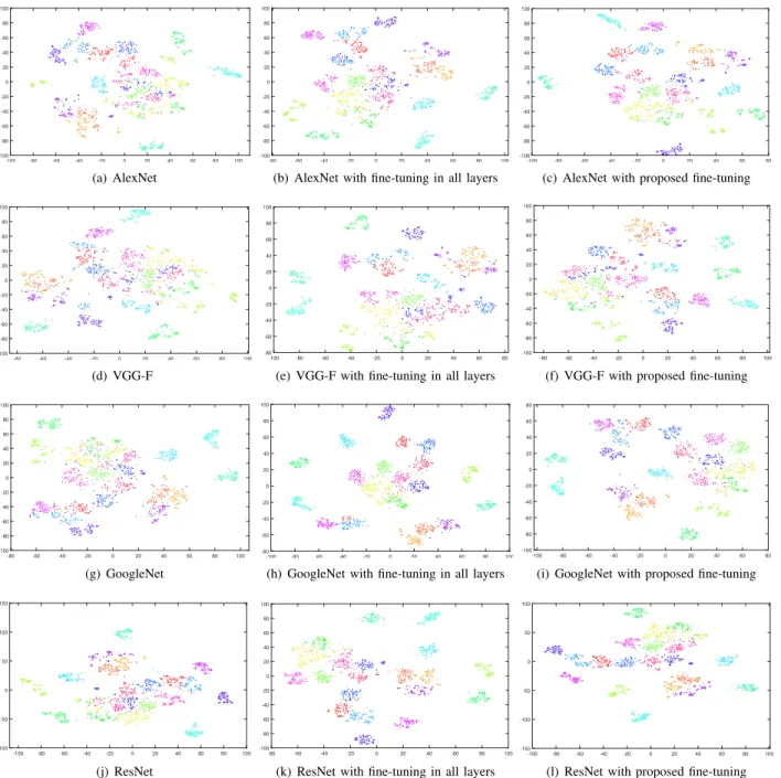
In order to qualitatively evaluate the performances of differ-ent features (pre-trained model, pre-trained model with tuning on all layers, pre-trained model with proposed fine-tuning method), we adopt the t-Distributed Stochastic Neigh-bor Embedding (t-SNE) algorithm proposed in [18] to visual-ize the feature distributions for different classes. The algorithm performs dimensionality reduction on high-dimensional data and, at the same time, preserves the significant structures of high-dimensional data. With all the CNN models available, we extract image features for the original image dataset with 2100 images and apply t-SNE to reduce these image features

to two dimensions. The scatter plots of these images in the corresponding reduced two-dimensional feature space are illustrated in Fig. 5. Each point in the plot represents an image in the dataset and different classes are indicated with different colors. From these plots, it is obvious to see that image features extracted from the proposed fine-tuning method tend to cluster better in the reduced two dimensional feature space than the features extracted using other two schemes, therefore it is easier to differentiate them using a designed classifier.

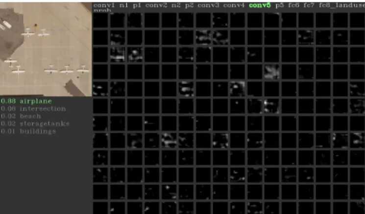
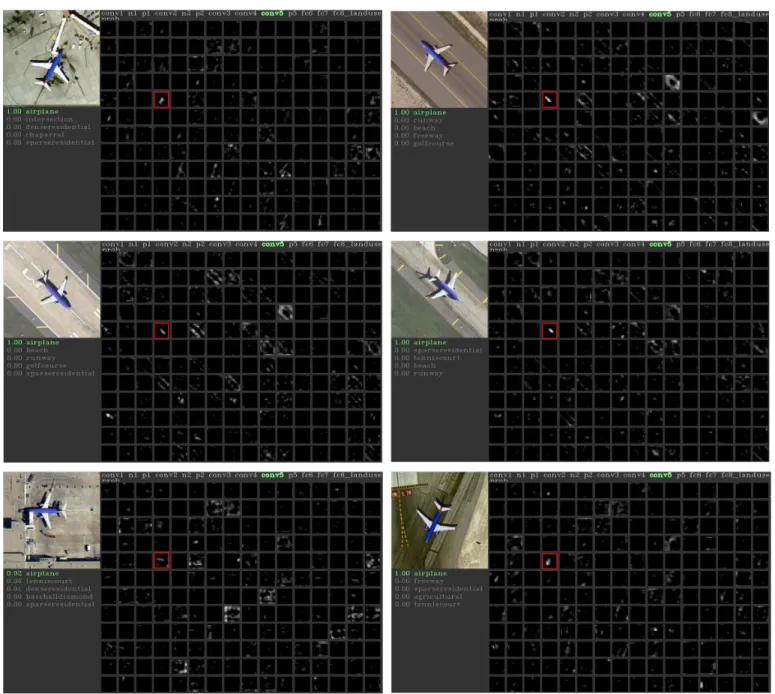
The other way to compare the performances of different CNN models is to visualize the filter weights and its corre-sponding activation outputs of various layers. We apply the toolbox provided by Yosinski et al. [19] for this purpose. In order to demonstrate the idea, an “airplane” image from the dataset is fed into the modified pre-trained AlexNet model, the fine-tuned AlexNet model using the traditional fine-tune method, and the fine-tuned AlexNet model with the proposed approach. For each layer of the network, the toolbox plots the learned weights and activation maps of the filters from different layers. Outputs from the low-level filters respond to edges and corners in the image while high-level filters from CONV5 create meaningful objects. The last layer of AlexNet contains 21 neurons, each one corresponds to the probability of the image being classified as a spacific class. The “CONV5” response using the proposed fine-tuned model is shown in Fig. 6. We also display the classification outputs from different CNN models in the same figure. According to these results, only the model from our proposed fine-tuning scheme correctly classify the image as an airplane (with probability of 0.88), while the other two methods classify the image as “intersection” with probability of 0.5 and 0.41 respectively, and consider it as an airplane with probability of 0.3. To better understand what what filters in “CONV5” layer learn from our dataset, we manually feed all the “airplane” image scenes from the UCMerced dataset [5] to the proposed fine-tuned AlexNet model and visualize the filter responses from “CONV5” layer. We observe that one of the neurons from “CONV5” layer obtains high response for image scenes with single blue plane, as indicated in Fig. 7. These responses also indicate that the neuron is capable to detect planes with different orientations.

V. DISCUSSION

One of the major difficulties regrading to training a deep neural network is to make sure that the trained neural network is not over-fitted on the training dataset. As a result, the drop out (DROP) layer was proposed in AlexNet and VGG-F to reduce the number of training parameters when learning CNN architectures. On the other hand, the GoogleNet and ResNet

-100 -80 -60 -40 -20 0 20 40 60 80 100 -100 -80 -60 -40 -20 0 20 40 60 80 100 (a) AlexNet -80 -60 -40 -20 0 20 40 60 80 100 -100 -80 -60 -40 -20 0 20 40 60 80 100

(b) AlexNet with fine-tuning in all layers

-100 -80 -60 -40 -20 0 20 40 60 80 -100 -80 -60 -40 -20 0 20 40 60 80 100

(c) AlexNet with proposed fine-tuning

-80 -60 -40 -20 0 20 40 60 80 100 -100 -80 -60 -40 -20 0 20 40 60 80 100 (d) VGG-F -100 -80 -60 -40 -20 0 20 40 60 80 -80 -60 -40 -20 0 20 40 60 80 100

(e) VGG-F with fine-tuning in all layers

-80 -60 -40 -20 0 20 40 60 80 100 -100 -80 -60 -40 -20 0 20 40 60 80 100

(f) VGG-F with proposed fine-tuning

-80 -60 -40 -20 0 20 40 60 80 100 -100 -80 -60 -40 -20 0 20 40 60 80 100 (g) GoogleNet -100 -80 -60 -40 -20 0 20 40 60 80 100 -80 -60 -40 -20 0 20 40 60 80 100

(h) GoogleNet with fine-tuning in all layers

-100 -80 -60 -40 -20 0 20 40 60 80 -100 -80 -60 -40 -20 0 20 40 60 80

(i) GoogleNet with proposed fine-tuning

-100 -80 -60 -40 -20 0 20 40 60 80 100 -100 -50 0 50 100 150 (j) ResNet -80 -60 -40 -20 0 20 40 60 80 100 -100 -80 -60 -40 -20 0 20 40 60 80 100

(k) ResNet with fine-tuning in all layers

-100 -80 -60 -40 -20 0 20 40 60 80 100 -150 -100 -50 0 50 100

(l) ResNet with proposed fine-tuning

Fig. 5: t-SNE visualization of different CNN features. First column: pre-trained CNN features without fine-tuning; Second column: pre-trained CNN with all-layer fine-tuning procedure; Last Column: pre-trained CNN with proposed fine-tuning procedure.

reduce the number of learning parameters by designing filters with smaller spatial receptive fields while at the same time extend the depth of the neural network. In the fine-tuning problem, data augmentation that generates more training im-ages is preferred for training a deep neural network. However, in this paper, we propose to reduce the number of training parameters by fine-tuning few layers of the CNN architecture, instead of the whole network. Through experiments on aerial image classification using the pre-trained CNN architectures, we argue that low levels of the pre-trained CNN architectures generalize well to other classification tasks. Therefore, we

argue that only higher levels of the architectures are needed for fine-tuning. In order to determine which layers are needed for fine-tuning, we carry out image classification experiments based on image features directly extracted from pre-trained CNN architectures. One possible reason for getting better results with less number of layers for fine-tuning is that a large number of training parameters are reduced, which is desirable given the small number of images in the dataset.

(a) Visualization of “CONV5” layer in proposed fine-tuned AlexNet, the test image is corrrectly classified

(b) Classification results from pre-trained Alex model(left) and conventional fine-tuned model(right).

Fig. 6: Visualization of activation from “CONV5” layer of “AlexNet” on an “airplane” image with deep visualization toolbox [19]

VI. CONCLUSION

In this paper, we propose a fine-tuning method for classi-fying high resolution aerial images based on pre-trained con-volutional neural network models. We first demonstrate that pre-trained CNN architectures from the ImageNet dataset is capable for generating good image features for high resolution aerial image classification. Based on our observations from the classification performance using pre-trained CNN models, we selectively apply transer learing methods that fine-tunes high-level layers of pre-trained CNN models, while keep the low-level layers unchanged. Our experimental results indicate that the pre-trained CNN features generalize well to high resolution remote sensing images and the proposed fine-tuning method performs better than existing fine-tuning schemes. In order to visualize the performance of our fine-tuned model, we investigate two existing visualization toolboxes to 1) observe the distribution of CNN features extracted from different CNN architectures, and 2) visualize the activation outputs of high-level layers, which correspond to semantic meaning of the image scene.

Future work would be focused on: 1) Explore fine-tuning

techniques that modify a small number of layers only, 2) Inves-tigate other data augmentation techniques for generating more images, in the hope of getting more layers involved during the fine-tuning process, 3) Visualize the differences between different fine-tuning methods and analyze the responses of different neurons for recognizing different scenes/objects.

ACKNOWLEDGMENT

The authors would like to thank Yangqing Jia et. al. for making the Caffe toolbox available online.

REFERENCES

[1] J. Huang, S. R. Kumar, M. Mitra, W.-J. Zhu, and R. Zabih, “Image indexing using color correlograms,” inIEEE Conf. on Comput. Vision and Pattern Recognition, San Juan, Pureto Rico, June, 1997, pp. 762– 768.

[2] M. J. Swain and D. H. Ballard, “Color indexing,”Int. J. of Comput. Vision, vol. 7, pp. 11–32, Nov. 1991.

[3] O. A. Penatti, K. Nogueira, and J. A. dos Santos, “Do deep features generalize from everyday objects to remote sensing and aerial scenes domains?” inIEEE Conf. on Computer Vision and Pattern Recognition Workshops, Boston, MA, Jun., 2015, pp. 44–51.

[4] O. Russakovsky, J. Deng, H. Su, J. Krause, S. Satheesh, S. Ma, Z. Huang, A. Karpathy, A. Khosla, M. Bernstein, A. C. Berg, and F.-F. Li, “Imagenet large scale visual recognition challenge,”Int. J. of Comput. Vision, vol. 115, pp. 211–252, Dec. 2015.

[5] Y. Yang and S. Newsam, “Bag-of-visual-words and spatial extensions for land-use classification,” inProc. of the 18th SIGSPATIAL Int. Conf. on Advances in Geographic Inform. Syst., San Jose, CA, Nov., 2010, pp. 270–279.

[6] S. Lazebnik, C. Schmid, and J. Ponce, “Beyond bags of features: Spatial pyramid matching for recognizing natural scene categories,” in IEEE Conf. on Comput. Vision and Pattern Recognition, New York, NY, June, 2006, pp. 2169–2178.

[7] S. Chen and Y. Tian, “Pyramid of spatial relatons for scene-level land use classification,”IEEE Trans. Geosci. Remote Sens., vol. 53, pp. 1947– 1957, Sept. 2015.

[8] F. Zhang, B. Du, and L. Zhang, “Saliency-guided unsupervised feature learning for scene classification,” IEEE Trans. Geosci. Remote Sens., vol. 53, pp. 2175–2184, Apr. 2015.

[9] W. Xiong, L. Zhang, B. Du, and D. Tao, “Combining local and global: Rich and robust feature pooling for visual recognition,”Pattern Recognition, vol. 62, pp. 225–235, Feb. 2017.

[10] A. Krizhevsky, I. Sutskever, and G. E. Hinton, “Imagenet classification with deep convolutional neural networks,” inAdvances in neural infor-mation processing systems, 2012, pp. 1097–1105.

[11] J. Deng, W. Dong, R. Socher, L.-J. Li, K. Li, and L. Fei-Fei, “ImageNet: A Large-Scale Hierarchical Image Database,” inIEEE Conf. on Comput. Vision and Pattern Recognition, Miami, FL, Aug. 2009, pp. 248–255. [12] K. Chatfield, K. Simonyan, A. Vedaldi, and A. Zisserman, “Return of

the devil in the details: Delving deep into convolutional nets,” inProc. of the British Machine Vision Conf., 2014.

[13] C. Szegedy, W. Liu, Y. Jia, P. Sermanet, S. Reed, D. Anguelov, D. Erhan, V. Vanhoucke, and A. Rabinovich, “Going deeper with convolutions,” in IEEE Conf. on Comput. Vision and Pattern Recognition, Boston, MA, June, 2015, pp. 1–9.

[14] K. He, X. Zhang, S. Ren, and J. Sun, “Deep residual learning for image recognition,” inIEEE Conf. on Comput. Vision and Pattern Recognition, Las Vagas, NV, June, 2016.

[15] P. Sermanet, D. Eigen, X. Zhang, M. Mathieu, R. Fergus, and Y. Le-Cun, “Overfeat: Integrated recognition, localization and detection using convolutional networks,” in Intel. Conf. on Learning Representations, Scottsdale, AZ, May, 2015.

[16] M. Castelluccio, G. Poggi, C. Sansone, and L. Verdoliva, “Land use clas-sification in remote sensing images by convolutional neural networks,” arXiv preprint arXiv:1508.00092, 2015.

[17] F. Hu, G.-S. Xia, J. Hu, and L. Zhang, “Transferring deep convolutional neural networks for the scene classification of high-resolution remote sensing imagery,”Remote Sensing, vol. 7, pp. 14 680–14 707, 2015. [18] L. v. d. Maaten and G. Hinton, “Visualizing data using t-sne,”Journal

Fig. 7: “CONV5” layer activation visualization of airplane scenes that contain a single blue airplane, filters indicated with red“ bounding-box” have high responses on different orientations of the airplane

[19] J. Yosinski, J. Clune, A. Nguyen, T. Fuchs, and H. Lipson, “Under-standing neural networks through deep visualization,” arXiv preprint arXiv:1506.06579, 2015.