Image Captioning with Recurrent Neural Networks

BRNO UNIVERSITY OF TECHNOLOGY

FACULTY OF INFORMATION TECHNOLOGY

DEPARTMENT OF COMPUTER GRAPHICS

AND MULTIMEDIA

FAKULTA INFORMAČNÍCH TECHNOLOGIÍ ÚSTAV POČÍTAČOVÉ GRAFIKY A MULTIMÉDIÍ

IMAGE CAPTIONING WITH RECURRENT NEURAL

NETWORKS

POPIS FOTOGRAFIÍ POMOCÍ REKURENTNÍCH NEURONOVÝCH SÍTÍ

MASTER’S THESIS

DIPLOMOVÁ PRÁCE

AUTHOR

Bc. JAKUB KVITA

AUTOR PRÁCE

SUPERVISOR

Ing. MICHAL HRADIŠ, Ph.D.

VEDOUCÍ PRÁCE

Abstract

In this work I deal with automatic generation of image captions by using multiple types of neural networks. Thesis is based on the papers from MS COCO Captioning Challenge 2015 and character language models, popularized by A. Karpathy. Proposed model is com-bination of convolutional and recurrent neural network with encoder–decoder architecture. Vector representing encoded image is passed to language model as memory values of LSTM layers in the network. This work investigate, whether model with such simple architecture is able to generate captions and how good it is in comparison to other contemporary solu-tions. One of the results is that the proposed architecture is not sufficient for any image captioning task.

Abstrakt

Tato práce se zabývá automatickým generovaním popisů obrázků s využitím několika druhů neuronových sítí. Práce je založena na článcích z MS COCO Captioning Challenge 2015 a znakových jazykových modelech, popularizovaných A. Karpathym. Navržený model je kombinací konvoluční a rekurentní neuronové sítě s architekturou kodér–dekodér. Vektor reprezentující zakódovaný obrázek je předáván jazykovému modelu jako hodnoty paměti LSTM vrstev v síti. Práce zkoumá, na jaké úrovni je model s takto jednoduchou architek-turou schopen popisovat obrázky a jak si stojí v porovnání s ostatními současnými modely. Jedním ze závěrů práce je, že navržená architektura není dostatečná pro jakýkoli popis obrázků.

Keywords

recurrent neural networks, RNN, convolutional neural networks, CNN, image captioning, LSTM, GRU, MS COCO, Torch, deep learning

Klíčová slova

rekurentní neuronové sítě, RNN, konvoluční neuronové sítě, CNN, popisování obrázků, LSTM, GRU, MS COCO, Torch, hluboké učení

Reference

KVITA, Jakub. Image Captioning with Recurrent Neural Networks. Brno, 2016. Master’s thesis. Brno University of Technology, Faculty of Information Technology. Supervisor Hradiš Michal.

Image Captioning with Recurrent Neural

Networks

Declaration

I hereby certify that this thesis is a presentation of my original research work and I have excercised reasonable care to ensure it does not to the best of my knowledge breach any law of copyright. Wherever contributions of others are involved, every effort is made to indicate this clearly, with due reference to the literature, and acknowledgement of collaborative research and discussions. The work was done under the guidance of Michal Hradiš at the Brno University of Technology.

. . . . Jakub Kvita May 11, 2016

Acknowledgements

Access to computing and storage facilities owned by parties and projects contributing to the National Grid Infrastructure MetaCentrum, provided under the programme “Projects of Large Research, Development, and Innovations Infrastructures”(CESNET LM2015042), is greatly appreciated.

c

○ Jakub Kvita, 2016.

This thesis was created as a school work at the Brno University of Technology, Faculty of Information Technology. The thesis is protected by copyright law and its use without author’s explicit consent is illegal, except for cases defined by law.

Contents

1 Introduction 4

2 Neural networks 5

2.1 Feed-forward neural nets . . . 5

2.2 Recurrent neural nets . . . 7

2.2.1 Recurrent architectures . . . 8

2.2.2 Modeling languages . . . 11

2.3 Convolutional neural nets . . . 12

3 Image Captioning 15 3.1 Related Work . . . 15 3.2 Datasets . . . 21 3.3 Evaluation. . . 22 3.3.1 Automated metrics . . . 22 4 Model design 24 4.1 Overall architecture . . . 24 4.1.1 Language model . . . 25

4.1.2 Hidden state initialization . . . 25

4.2 Training . . . 26 5 Implementation 28 5.1 Tools . . . 28 5.1.1 Torch . . . 29 5.2 Dataset MS COCO . . . 30 5.3 Model implementation . . . 31 5.3.1 Training . . . 32

5.4 Bag of Words experiments . . . 34

6 Experiments 35 6.1 Pretraining RNN . . . 36

6.2 Language model initialization variations . . . 37

6.3 Bag of Words experiments . . . 38

7 Conclusion 40

Bibliography 41

Appendices 47

List of Appendices . . . 48

A CD Contents 49

B MS COCO Annotation format 50

C Installing Torch 51

D Scripts Manuals 52

D.1 RNN pretraining . . . 52

D.2 Full model. . . 52

List of Figures

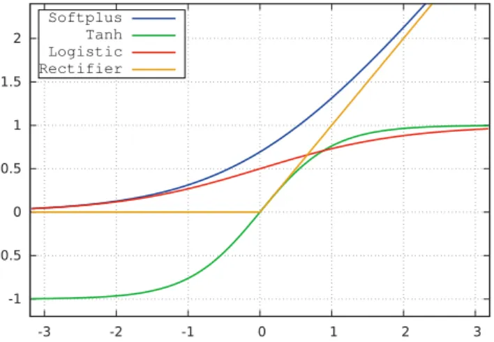
2.1 Nonlinear functions used in neural nets. . . 6

2.2 Applying dropout to a neural network. . . 7

2.3 Unrolling of a recurrent neural net. . . 8

2.4 Variation of a LSTM. . . 9

2.5 Variation of a GRU. . . 10

2.6 Architecture of famous CNNLeNet-5. [36] . . . 13

3.1 Show and Tell image captioning model. [54] . . . 17

3.2 From Captions to Visual Concepts caption generation pipeline. [14] . . . . 18

3.3 Show, Attend and Tell model architecture. [57] . . . 19

3.4 Examples ofShow, Attend and Tell attention. [57] . . . 20

3.5 The LRCN model architecture for video processing. [11] . . . 20

4.1 Architecture of the proposed model. . . 25

6.1 Distribution of caption lengths in the training data. . . 35

6.2 Pretrained RNN error based on character position in sequence. . . 36

6.3 Error of RNN initialized with CNN based on character position in sequence. 38

Chapter 1

Introduction

When does a machine understand an image? One definition could be the following sentence:

A machine understand an image, when it can describe important content of the image. This description should include present objects, their attributes and relation to each other. De-termining the important content of the image can be quite difficult, even for humans, which have been trained for this task since they were born. However, deep learning techniques are proving to be quite successful in this kind of tasks. Similarly to people, these mod-els require large amounts of training data, but, being properly trained, they can evaluate correctly even yet unseen situations.

Neural networks, sometimes mentioned under the name of deep learning, are a branch of machine learning based on composing multiple non-linear functions to solve the task. As it is fundamentally different from the standard computer algorithms, it perform well on problems, which are unsuitable for traditional solutions. For example, neural networks have excellent performance in recognizing speech and images, writing stories and composing music. This work focuses on generating image descriptions in regular English sentences, which is also a task suitable for deep learning.

This work consists of 7 chapters in total. Firstly, chapter 2 introduces neural networks and several key concepts, which are used later in this work. In chapter3 current state-of-the-art in the field of image captioning and summary of the key works will be presented. Equipped by knowledge from previous chapters, I will propose an image captioning model in chapter 4. Overview of the programming tools used for implementing neural nets is in chapter 5, as well as description of implementation of my model. Chapter 6 discusses ex-periments performed with my model, their results, and evaluation of the proposed solution. The concluding chapter7 serves as summary of the thesis and the important findings.

Chapter 2

Neural networks

General idea of artificial neural networks emerged after World War II. Perceptron, a single artificial neuron, was created in 1958 by Frank Rosenblatt [46], but it became popular only after combination with the backpropagation algorithm [5, 55]. At that time neural nets have not reached massive popularity, not because they do not work, but because small computing power of machines back then, and also the lack of datasets. Recently (after 2000), neural nets became popular again under the name of “deep learning” to emphasize the use of several layers stacked on top of each other to create deep architectures, which are far more practical than shallow ones. During this reinvention, neural nets have been successfully applied in multiple fields like computer vision [21], speech recognition [18], and natural language modeling [40].

Nowadays, various useful architectures, techniques and applications of neural nets are introduced almost every day. As it is not possible to through all of them, in this chapter I will describe only a handful, which are most significant and will be later used in the research. This chapter is divided into three sections, each focusing on different type of neural nets – feed-forward, recurrent, and convolutional. However, do not see this division as strict and separating, tools introduced in one part can and will be used in different types of networks.

2.1

Feed-forward neural nets

Feed-forward networks are simplest architecture of neural nets, yet they can solve many real world tasks. Most commonly used in classification problems, feed-forward nets showed very promising results, which later proved to be true. Later, they have been replaced by convolutional nets, which are specific type of complex feed-forward neural net. However, simple architectures still have place for utilization.

In this part I will cover linear neuron, rectifiers and other nonlinear functions used, and dropout, as they are most important to the following work. Other tools like softmax layer, loss functions, and training algorithms will be skipped.

Linear unit

In this type of neuron, the output of the unit is simply the weighted sum of its inputs added to a bias term, described by equation

-1 -0.5 0 0.5 1 1.5 2 -3 -2 -1 0 1 2 3 Softplus Tanh Logistic Rectifier

Figure 2.1: Nonlinear functions used in neural nets.

A combination of these neurons performs a linear transformation of the input vector. Ability to perform only linear and affine transformations is also its weakness, as some kind of nonlinear function needs to be added to produce more complicated functions. However it is useful at the beginning and end of the network, to emphasize important features of the input or output and change its dimensionality.

This type of unit is the most basic one. It was part of the Rosenblatt’s perceptron [46] as well as the boolean function, which later evolved into nonlinear functions, like Rectifier described further.

Rectifier and ReLU

Combination of linear layers in neural network can result only in another linear layer, which is useless for example on problems of nonlinear separation. To break free from limitations induced, we need to introduce some kind of nonlinearity directly into the network. Most commonly used method is to apply a nonlinear activation function to the output of a linear neuron. As to which function, there are many suitable options, rectifier nowadays being the most popular one.

In the context of neural networks, the rectifier is an activation function defined as

𝑓(𝑥) = 𝑚𝑎𝑥(0, 𝑥). (2.2)

Rectifier is usually used after a linear unit creating together Rectified Linear Unit (ReLU), which showed improvements in restricted Boltzmann machines [43], speech processing [59], and it is also default option in convolutional networks. This unit has several advantages against other functions – in randomly initialized networks, only about 50% of units are activated. There are no problems with vanishing gradient in large inputs. Computation of the function is also more efficient than other functions. Issue with this function is non-differentiability at zero, however it is differentiable at any point arbitrarily close to 0 and can be replaced with softplus [12], which is analytic function smoothly approximating rectifier. Currently, more variations of ReLU were introduced – Leaky ReLU, parametric ReLU, etc. and their performance can be even better [56] than vanilla ReLUs.

Before ReLU, popular functions were hyperbolic tangent and standard logistic function. However, these functions are costly to compute, even though they can be replaced with

(a) Standard neural net. (c) At training time. Present with

probability p.

w

(b) Applying dropout. (c) At test time. Always

present.

pw

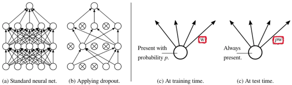
Figure 2.2: Applying dropout to a neural network.

polynomials. Hyperbolic tangent was preferred as better version of logistic function [37]. See how the discussed functions look at Figure2.1.

Dropout

Dropout [22, 49] can be considered as one of the biggest recent inventions in the field of neural networks. It is extremely simple and effective technique addressing the problem of overfitting. It can be seen as type of regularization, together with techniques like L1 and L2 regularization, and constraining maximum value of weights.

Dropout works with the idea of “dropping out” some of the unit activations in a layer, that is setting them to zero, during training. This can be interpreted as sampling a neural network from the full neural network, and only updating the parameters of the sampled network for the given data. Visualisation is on Figure2.2, partsa andb. Dropout behaves differently during sampling phase – all the units are present, but their outputs are multiplied by the same probability used before for dropping them out. See the partc andd of Figure

2.2.

This technique should prevent complex co-adaptations, in which unit is only helpful in the context of several other specific units. Each neuron instead learns to detect a feature generally useful for computing the answer.

2.2

Recurrent neural nets

Feedforward neural nets are extremely powerful models, but they can be only applied to problems with inputs and outputs of fixed dimensionality. This is a serious drawback, as many of the real-world problems are defined as sequences with lengths that are unknown to us beforehand. Recurrent neural networks were introduced soon after feed-forward nets and they proved to be very useful in this kind of a task. There is vast amount of recurrent neural network types, many not suitable for sequential tasks, like Hopfield networks [26], which are very successful in what they do, but nevertheless not useful for us now.

Apart from classification, which can be more precise when using sequences, one of the most important tasks is next value prediction. This core task can be then extended very simply to predict arbitrary number of future values. Prediction problems are all around us, from the weather forecast and stock market prediction to the autocomplete in smartphones or web browsers. The image captioning problem, which is the main topic in this work, includes the prediction (or generation) task too, as the caption is generated one character at a time starting from the “base caption”. Detailed description is in the following chapters.

=

A

A

A

A

A

Figure 2.3: Unrolling of a recurrent neural net.

We can interpret recurrent neural network as very deep forward net with shared weights and same inputs and outputs as before. This process of reinterpreting the network is called RNN unrolling and is visualised in Figure2.3. Layers of this very deep net spread forward in time, together with the input sequence. This is very innovative idea, which enabled training RNN with backpropagation through time, as we are not bound by time during training.

Unrolling the networks on long sequences and creation of very deep neural nets caused manifestation of the vanishing gradient problem, which is one of the most important is-sues in RNNs. The problem occurs during training with gradient-based learning methods like backpropagation. The chain rule in backpropagation multiplies gradients to compute updates of weights and the traditional activation functions like hyperbolic tangent have gradient in the range of (₋1,1), are the reasons why, the weights updates decrease expo-nentially while approaching front layers of the network. The vanishing gradient problem was formally identified by Hochreiter in 1991 [23], who, after further research, also proposed one of the solutions to this problem in the form of Long Short-Term Memory.

Long Short-Term Memory unit and other architectures commonly used in RNNs are discussed in following section2.2.1. Second half (2.2.2) of this part explains how to process text and model languages for applications with RNNs.

2.2.1 Recurrent architectures

RNNs have many different architectures, however, most of them are derived from the basic fully recurrent network. This network do not have units separated into layers, as each of them has a directed connection to every other unit. Rest of the architectures are special cases of this one, as they group neurons into layers and implement only a subset of the connections. Examples of these architectures can be Hopfield [26] and Elman [13] networks, and Restricted Boltzmann Machines [48]. Different architectures are trying to connect RNN with an external memory resource, which can be a tape in case of Neural Turing Machines [19], a stack in Neural network Pushdown Automata [50], etc. During training RNN unrolling can be applied to these architectures, although training can be quite difficult, as explained earlier.

From here on in I will focus on an architecture called Long Short-Term Memory and ar-chitectures derived from it, as they are very powerful and dominating the current field.These units are carefully designed with the vanishing gradient problem in mind and perform better than most of the other architectures.

σ w w w σ w w w tanh w w tanh

+

+

x

x

x

h

h

h

C

C

f

i

C

o

Long Short-Term Memory

Long Short-Term Memory (LSTM) is a special type of recurrent network, able to learn long-term dependencies. This architecture was introduced by Hochreiter and Schmidhuber [24] after prior research of vanishing gradient problem, and later refined and popularized by other researchers [15,16].

LSTM was designed to remember a value for an arbitrary length of time. It contains gates that determine, when the input is significant enough to remember, when it should keep or forget the value, and when it should copy the value to the output. To understand the flow of data, see the diagram of LSTM on Figure 2.4. All the gates can be described by the following equations:

𝑖𝑡 = 𝜎(𝑊𝑥𝑖𝑥𝑡+𝑊ℎ𝑖ℎ𝑡−1+𝑊𝑐𝑖𝐶𝑡−1+𝑏𝑖) (2.3) 𝑓𝑡 = 𝜎(𝑊𝑥𝑓𝑥𝑡+𝑊ℎ𝑓ℎ𝑡−1+𝑊𝑐𝑓𝐶𝑡−1+𝑏𝑓) (2.4) ̃︀ 𝐶𝑡 = tanh(𝑊𝑥𝑐𝑥𝑡+𝑊ℎ𝑐ℎ𝑡−1+𝑏𝑐) (2.5) 𝐶𝑡 = 𝑓𝑡⊙𝐶𝑡−1+𝑖𝑡⊙𝐶̃︀𝑡 (2.6) 𝑜𝑡 = 𝜎(𝑊𝑥𝑜𝑥𝑡+𝑊ℎ𝑜ℎ𝑡−1+𝑊𝑐𝑜𝐶𝑡+𝑏𝑜) (2.7) ℎ𝑡 = 𝑜𝑡⊙tanh(𝐶𝑡) (2.8) 𝜎(𝑥) = 1 1 +𝑒−𝑥 (2.9)

In each time slice LSTM is using current input𝑥𝑡, last cell state𝐶𝑡−1 and unit outputℎ𝑡−1

to compute next cell state𝐶𝑡and outputℎ𝑡. Variables𝑖𝑡,𝑓𝑡,𝑜𝑡denote values of in following

order input, forget and output gates, which are used to control the information flow. LSTM based on these equations is using total of 11 weight matrices, 4 bias vectors, and a standard logistic function𝜎 defined in Equation (2.9). The operation_⊙denotes element-wise vector product.

Equations (2.3) to (2.9) are not the only way to create an LSTM unit, they are a variation, which was used for implementing the proposed model. As LSTM is very popular,

h

x

h

h

+

x

x

r

z

x

h

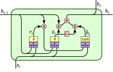
Figure 2.5: Variation of a GRU.

many different forms were created. For example, original LSTM from 1997 [24] did not included the “peephole connections” 𝑊𝑐𝑖𝐶𝑡−1, 𝑊𝑐𝑓𝐶𝑡−1, and 𝑊𝑐𝑜𝐶𝑡. These were added

later in work of Gers and Schmidhuber [15]. Another change is to couple input gate 𝑖𝑡

and forget gate 𝑓𝑡. Instead of separately deciding what to forget and when to input new

information, unit only forgets the value when something new is placed in its place. More units based on LSTM and their comparison is in work of Greff, et al. [20].

Training of the LSTM based network can be performed effectively by standard meth-ods like stochastic gradient descend in the form of backpropagation through time. Major problem with vanishing gradients during training described earlier is not an issue as back-propagated error is fed back to each of the gates.

Gated Recurrent Unit

Gated Recurrent Unit (GRU) [7] is slightly more dramatic variation on the LSTM theme. It combines hidden state of the unit ℎ𝑡 with the saved value 𝐶𝑡, merges input and forget

gates into one update gate𝑧𝑡and some smaller changes. Compare GRU diagram on Figure

2.5with the previous LSTM figure. GRU is based on following set of equations:

𝑟𝑡 = 𝜎(𝑊𝑥𝑟𝑥𝑡+𝑊ℎ𝑟ℎ𝑡−1+𝑏𝑟) (2.10)

𝑧𝑡 = 𝜎(𝑊𝑥𝑧𝑥𝑡+𝑊ℎ𝑧ℎ𝑡−1+𝑏𝑧) (2.11)

̃︀

ℎ𝑡 = tanh(𝑊𝑥ℎ𝑥𝑡+𝑊ℎℎ(ℎ𝑡−1⊙𝑟𝑡) +𝑏ℎ) (2.12)

ℎ𝑡 = (1−𝑧𝑡)⊙̃︀ℎ𝑡+𝑧𝑡⊙ℎ𝑡−1 (2.13)

On top of the Equations (2.10) to (2.13), GRU is using the standard logistic function 𝜎 defined in Equation (2.9). The operation_⊙again denotes the element-wise vector product. As the unit is using only 4 weight matrices, 3 biases and 1 state variable, researchers studied whether it can achieve the performance on same level as previous LSTM.

In Chung’s study [8], different types of recurrent units were compared on the polyphonic music datasets. LSTM and GRU were performing significantly better than all of the other architectures, with GRU slightly in the lead. According to Greff, et al. [20] on the other

hand, GRU is an average variation, slightly better than vanilla LSTM, with much simpler architecture.

Jozefowicz’s study [30] tried to determine whether the LSTM architecture is optimal and if such architecture exists. On variety of tasks and the data GRU outperformed LSTM on all tasks with the exception of language modeling. On top of that, they identified architectures that outperforms both LSTM and GRU. These architectures were found by evolutionary algorithm working on candidate architectures represented by the computational graph. In this work I will explore different type of language modeling than the one used in Jozefowicz’s paper [30] and I will not focus on these new types of units. Interestingly they also confirmed that LSTM nearly matched the GRU’s performance, when its forget gate bias was initialized to a large value such as 1 or 2, and not to naive initialization around 0. This idea was already presented by Gers [16] and can be interpreted in a way that LSTM will not explicitly forget anything until it has learned to forget.

Generally, researchers agree that most of the LSTM variations, including GRU, are roughly on the same performance level. As the changes introduced in GRU are simplifying the standard LSTM model even though keeping the performance level, GRU has been growing increasingly popular.

2.2.2 Modeling languages

With the addition of LSTM, recurrent neural nets quickly showed great potential in many different types of sequence processing like speech recognition, signal prediction and modeling languages. These result were further improved when researchers started stacking LSTMs on top of each other. Language modeling has several ways to process input text and feed it to the network. In this chapter, I will describe word and character level models, which are most commonly used.

Word level representation of the text is used by most of the state-of-the-art models, have been enhanced by many features and proved very effective for English. In this method, each word is encoded to a vector of a constant length. The neural network then works only with these encodings and does not have direct access to the word and its form. The advantage of this approach is no need to teach the model exact spelling of the words, which also means the model is not going to be confused by homographs1. The benefit also is that encoded sequences are much shorter than sequences based on dividing text by character. On the other hand, the disadvantage of this approach is that modeling non-word text, like punctuation and long numbers, can be complicated.

All that is left, is to decide specific encoding for model to use. Simple way that comes to mind is one-hot2 or one-from-k encoding, which has its advantages, however, there are several issues with it in this application. The task vocabulary often exceeds 100 000 records, which means each input vector would be incredibly long. So long, issues with time complex-ity of computations would appear. Luckily set of techniques called word embedding were developed.

Word embedding [3] is a tool for mapping words or phrases from the vocabulary to suitable vectors of real numbers in low dimensional space (around 200 – 500 dimensions)

1_{Ahomograph is a word that shares the same written form as another word but has a different meaning.}

2

relative to the vocabulary. For example,

𝑊(ℎ𝑜𝑟𝑠𝑒) = (0.2, 0.4, 0.7, 0.1, . . .), (2.14) 𝑊(𝑤𝑖𝑛𝑑𝑜𝑤) = (0.0, 0.6, 0.1, 0.9, . . .). (2.15) Vectors are usually randomly initialized and then trained to capture structure of the input data to perform some task. An example can be skip-gram model [39], which mapped 783 millions words to vectors of 300 real numbers, while creating reasonable relationships between them. Word embeddings show many interesting properties, like encoding analogies between words as differences between their vectors [41], but I am not going to cover them in more detail in this work.

Character level modeling has been considered as an alternative to word-level, but so far had worse performance. Regardless, it is still considered as an option, because of the much simpler representation of the input and output. Consider roughly45 characters in English text and over 100000 words created from them. Same input can be modeled in character level by simple one hot encoding, instead of creating whole field of the word embeddings. These models are also more suited for Czech, Russian, and other fusional3languages, which heavily use prefixes and suffixes to create new words.

Character level models usually have smaller vocabulary size and tend to take more time for training, as they need to learn spelling of the words and structure of a sentence, on top of the same features of word level. However, with the properly trained character level model, we can benefit from its greater generative abilities, on top of the very simple input and output of the model.

2.3

Convolutional neural nets

Feed-forward neural nets together with backpropagation algorithm have showed very useful for range of tasks and it has been even proven [9,27] they can approximate any continuous function. However, they are not very good in recognizing objects presented visually. As every unit is connected to large amount of units in the previous layer (or all of them in fully-connected layers), the number of weights grows rapidly with the size of the problem and even more with the dimensionality. All these issues are becoming apparent even in image processing, which has only two dimensions. Convolutional neural nets (CNN) were introduced as a way to reduce the number of parameters involved, while exploiting the spatial constraints of the input.

CNN ideas took inspiration from neurobiology, more precisely the organisation of neu-rons in visual cortex of the cat. They were first used in the work of Homma [1], to process a temporal signal, and their design was later improved by LeCun et al. [36]. Different CNN architecture was proposed by Graupe [17] for decomposing one-dimensional EMG signals4. Convolutional nets can be also used in natural language processing [33] and analysis of three-dimensional data like videos [29] or volumetric data (e.g. 3D medical scans), but that is not as common as image processing.

Basic architecture of CNN can be described by the following process:

3

Fusional language is a type of language distinguished by its tendency to overlay many morphemes to denote grammatical, syntactic, or semantic change.

4

Electromyography (EMG) is an electrodiagnostic medicine technique for evaluating and recording the electrical activity produced by muscles.

INPUT 32x32 Convolutions Subsampling Convolutions C1: feature maps 6@28x28 Subsampling S2: f. maps 6@14x14 S4: f. maps 16@5x5 C5: layer 120 C3: f. maps 16@10x10 F6: layer 84 Full connection Full connection Gaussian connections OUTPUT 10

Figure 2.6: Architecture of famous CNNLeNet-5. [36]

1. Convolve several small filters on the input. 2. Subsample this space of filter activations.

3. Repeat steps 1 and 2 until you are left with a sufficiently high level features. 4. Use a standard feed-forward neural net to solve the task, using the features

from step 3as input.

Thus the CNN consist of alternating convolutional and subsampling layers, followed by fully-connected feed-forward network. Diagram of the simple CNN architecture is on Figure

2.6. I will now go through the individual network segments and describe them.

Convolutional layer, which is most important and gave CNNs their name, is essentially the same as mathematical convolution used elsewhere. Here it means to apply a ’filter’ over an input at all possible offsets. This filter - in image processing and computer vision called kernel - has a layer of connection weights with the same dimensionality as the input, but with much smaller size. Despite the fact that there is many connections in one convolution, which are even overlapping, the weights are tied together and only handful of parameters per filter need to be updated during training. Usually, several filters, ranging from 5 to 100, are applied to the input simultaneously in one layer. The main reason why it is possible to use this architecture is the ability to stack convolutions on top of each other to create more high-level from low-level features, while keeping the proportions of input.

As the output of the network usually do not have same dimensions of the input, ability to directly control size of the features is needed. In CNNs it is provided by subsampling, or in this version max pooling, layer. It is a simple operation that takes small non-overlapping grid of the input tensor and outputs the maximum value of each part. By putting this operation in between the convolutional layers, we can scale the current feature tensor and detect higher level features than without it.

Nowadays, most popular way to introduce nonlinearity to CNN is inserting rectifiers after convolutions, as they have excellent performance, surpassing any other unit [28, 43]. In the second, fully-connected part, mix of linear units and ReLUs is commonly used, with applying dropout to these layers. Connection between convolutional and fully-connected part is provided by a layer converting higher-dimensional output data from convolutions to a one-dimensional input vector.

CNNs are useful in applications, where data has a spatial structure, which is useful to capture in the model. Among these data belongs image processing and speech recognition. One of the first and most famous examples of convolutional neural net is LeNet5[36], which recognize handwritten digits from the MNIST database6. Figure2.6shows the architecture of LeNet, version calledLeNet-5.

5

Demos and examples of LeNet: http://yann.lecun.com/exdb/lenet/

6

Chapter 3

Image Captioning

Scene understanding is one of the fundamental, but also most difficult tasks of computer vision and ability to automatically generate text captions of an image or video can have a great impact on lives of many. However, it is much more complicated than simple clas-sification or object recognition tasks, because the model also need to understand relations between the recognized objects and encode that relationship correctly in the caption.

In this chapter, I have done an overview of state-of-the-art approaches to the image captioning task and more closely describe latest studies, which are the basis of this work (section3.1). Following section 3.2cover popular datasets. Last section3.3 covers evalua-tion procedures, which are most commonly used for this task.

3.1

Related Work

Two main approaches to image captioning were popular, until neural networks dominated the field. The first one used caption templates, which were filled by detected objects and relations. Second was based on retrieval of similar captions from database and modifying them to fit the current image. Question of similarity ranking has been addressed by many papers, which are based on the idea of joint embedding vector space for both images and captions [32], as it transforms estimation of similarity to a simple proximity measurement. Both approaches included a generalization step to remove information relevant only to current image, for example names.

These approaches were quite successful in describing images, but they are heavily hand-designed. Also their text-generation power is fixated on the database/embeddings and is not able to describe previously unseen compositions of objects. Over time these approaches fell out of favor, as methods leveraging the power of neural networks emerged. However, some of their ideas proved to be useful in the new environment and we can encounter them in recent works [14].

Many of the new methods, which use neural nets, are inspired by the success in training recurrent nets for machine translation. It is worth mentioning Sutskevers work [51], which studied general sequence to sequence mapping by converting an input sequence to the fixed length vector, which is then decoded to the output sequence. This encoder–decoder archi-tecture is closely related to the autoencoders and work of Kalchbrenner and Blunsom [31], who were first to map the entire input sequence to vector.

The introduced encoder–decoder architecture is important to the captioning task, be-cause image description problem can be interpreted as a translation from an image to a

sentence. In this case, encoder part of the model is usually a convolutional neural net, as they are excellent in the image classification [52]. Decoder part is the similar to the one in machine translation models – an RNN or a type of LSTM, as the output for both tasks is essentially the same.

Following the encoder–decoder idea, current image captioning research is shifting to-wards models, which are trained end-to-end with some type of stochastic gradient descent (SGD) algorithm. The reasons for the shift can be simplicity and a lot less hand design than in other methods. Different type of the state-of-the-art models are based on proven pipeline of key-word detection, sentence generation, and ranking, which exploit the power of embedded neural networks, which specialize in single task. This approach is more closely described in section discussing article From Captions to Visual Concepts and Back.

The current field is consolidating, thanks to MS COCO Captioning Challenge1 and dataset created for it. Simple public access to the necessary data makes model creation easier and the best researchers can compete directly against each other by using MS COCO evaluation server. In the rest of this section, I describe several works, which were submitted to the challenge in 2015 and had the best performance. MS COCO dataset is described, together with other datasets, in following section 3.2.

Show and Tell: A Neural Image Caption Generator

Show and Tell [54] is model created by Google researchers, which tied for the first place in MS COCO Captioning Challenge with the following model From Captions to Visual Concepts. The main idea of this work is to use recent advancements in machine translation and apply them for image captioning. Model uses encoder–decoder architecture, with CNN for the encoder part and RNN for the decoder part, as described earlier. Model is trained to maximize the likelihood𝑝(𝑆_|𝐼)of producing a target sequence of words 𝑆=_{𝑆1, 𝑆2, ...}

given an input image𝐼.

Used convolutional neural net has been pre-trained for an image classification task and last hidden layer of this network has been used as an input to the RNN decoder. The RNN part of the network is made of LSTM units based on following equations:

𝑖𝑡 = 𝜎(𝑊𝑥𝑖𝑥𝑡+𝑊ℎ𝑖ℎ𝑡−1) (3.1) 𝑓𝑡 = 𝜎(𝑊𝑥𝑓𝑥𝑡+𝑊ℎ𝑓ℎ𝑡−1) (3.2) ̃︀ 𝐶𝑡 = tanh(𝑊𝑥𝑐𝑥𝑡+𝑊ℎ𝑐ℎ𝑡−1) (3.3) 𝐶𝑡 = 𝑓𝑡⊙𝐶𝑡−1+𝑖𝑡⊙𝐶̃︀𝑡 (3.4) 𝑜𝑡 = 𝜎(𝑊𝑥𝑜𝑥𝑡+𝑊ℎ𝑜ℎ𝑡−1) (3.5) ℎ𝑡 = 𝑜𝑡⊙𝐶𝑡 (3.6)

Notation is same as in the chapter2,𝜎 is the standard logistic function defined in Equation (2.9) and the operation _⊙ denotes the element-wise vector product. It is worth noticing the LSTM version used do not have “peephole connections”. Several more changes were added – the second evaluation of hyperbolic tangent in Equation (3.6) is missing, as well as biases in all equations.

The language model is working on the word-level, part of the RNN is word embed-ding [39], which is trained together with the model. CNN, which is used to generate a configuration vector from the image, is connected to the RNN at the beginning as the first

1

LSTM LSTM LSTM WeS1 WeSN-1

p1 p2 pN

log p1(S1) log p2(S2) log pN(SN)

...

Figure 3. LSTM model combined with a CNN image embedder

(as defined in [12]) and word embeddings. The unrolled

connec-tions between the LSTM memories are in blue and they

corre-spond to the recurrent connections in Figure 2. All LSTMs share

the same parameters.

image and each sentence word such that all LSTMs share

the same parameters and the output

m

of the LSTM at

time

t

−

1

is fed to the LSTM at time

t

(see Figure 3). All

recurrent connections are transformed to feed-forward

con-nections in the unrolled version. In more detail, if we denote

by

I

the input image and by

S

= (

S

, . . . , S

)

a true

sen-tence describing this image, the unrolling procedure reads:

x

=

CNN

(

I

)

(10)

x

=

W

S

,

t

∈ {

0

. . . N

−

1

}

(11)

p

=

LSTM

(

x

)

,

t

∈ {

0

. . . N

−

1

}

(12)

where we represent each word as a one-hot vector

S

of

dimension equal to the size of the dictionary. Note that we

denote by

S0

a special start word and by

S

a special stop

word which designates the start and end of the sentence. In

particular by emitting the stop word the LSTM signals that a

complete sentence has been generated. Both the image and

the words are mapped to the same space, the image by using

a vision CNN, the words by using word embedding

W

.

The image

I

is only input once, at

t

=

−

1

, to inform the

LSTM about the image contents. We empirically verified

that feeding the image at each time step as an extra input

yields inferior results, as the network can explicitly exploit

noise in the image and overfits more easily.

Our loss is the sum of the negative log likelihood of the

correct word at each step as follows:

L

(

I, S

) =

−

X

t=1

log

p

(

S

)

.

(13)

The above loss is minimized w.r.t. all the parameters of the

LSTM, the top layer of the image embedder CNN and word

Inference

There are multiple approaches that can be used

to generate a sentence given an image, with NIC. The first

one is

Sampling

where we just sample the first word

ac-cording to

p1, then provide the corresponding embedding

as input and sample

p

the special end-of-sentence token or some maximum length.

The second one is

BeamSearch

: iteratively consider the set

of the

k

best sentences up to time

t

as candidates to generate

sentences of size

t

+ 1

, and keep only the resulting best

k

of them. This better approximates

S

= arg max

p

(

S

|

I

)

.

We used the BeamSearch approach in the following

experi-ments, with a beam of size 20. Using a beam size of 1 (i.e.,

greedy search) did degrade our results by 2 BLEU points on

average.

4. Experiments

We performed an extensive set of experiments to assess

the effectiveness of our model using several metrics, data

sources, and model architectures, in order to compare to

prior art.

4.1. Evaluation Metrics

Although it is sometimes not clear whether a description

should be deemed successful or not given an image, prior

art has proposed several evaluation metrics. The most

re-liable (but time consuming) is to ask for raters to give a

subjective score on the usefulness of each description given

the image. In this paper, we used this to reinforce that some

of the automatic metrics indeed correlate with this

subjec-tive score, following the guidelines proposed in [11], which

asks the graders to evaluate each generated sentence with a

scale from 1 to 4

.

For this metric, we set up an Amazon Mechanical Turk

experiment. Each image was rated by 2 workers. The

typ-ical level of agreement between workers is

65%

. In case

of disagreement we simply average the scores and record

the average as the score. For variance analysis, we perform

bootstrapping (re-sampling the results with replacement and

computing means/standard deviation over the resampled

re-sults). Like [11] we report the fraction of scores which are

larger or equal than a set of predefined thresholds.

The rest of the metrics can be computed automatically

assuming one has access to groundtruth, i.e. human

gen-erated descriptions. The most commonly used metric so

far in the image description literature has been the BLEU

score [25], which is a form of precision of word n-grams

between generated and reference sentences

. Even though

1 _{The raters are asked whether the image is described without any}

er-rors, described with minor erer-rors, with a somewhat related description, or with an unrelated description, with a score of 4 being the best and 1 being the worst.

2_{In this literature, most previous work report BLEU-1, i.e., they only}

compute precision at the unigram level, whereas BLEU-n is a geometric

Figure 3.1: Show and Tell image captioning model. [54]

input before the generated sequence. Overall structure of the model is visualized on Figure

3.1and can be represented by following equations:

𝑥−1 = 𝐶𝑁 𝑁(𝐼) (3.7)

𝑥𝑡 = 𝑊𝑒𝑆𝑡 𝑡∈ {0. . . 𝑁−1} (3.8)

𝑝𝑡+1 = 𝐿𝑆𝑇 𝑀(𝑥𝑡) 𝑡∈ {0. . . 𝑁−1} (3.9)

As the image and word encodings are used in the same way, model is effectively mapping both images and words into the same vector space. During the sequence input, special start word𝑆0 and stop word 𝑆𝑁 designated to mark start and end of the sequence are used.

The CNN component of the model has been initialized to an ImageNet trained model, which helped quite a lot in terms of generalization. Word embeddings were left uninitialized (initialized randomly) as they did not observed significant gains while using large corpus. Dropout and ensebling used during training gave minor improvements. Model has been trained using SGD with fixed learning rate and no momentum. For the embeddings vector and the LSTM memory 512 dimensions were used. During the inference, beam search has been used to improve the results.

From Captions to Visual Concepts and Back

This work [14] took quite a different approach than a previous one, however, both tied for the first place in the captioning competition. This model is not trained end-to-end with a single training algorithm rather it has three connected stages. Full pipeline of the model is on the Figure 3.2and its description follows.

First, model learns to extract nouns, verbs, and adjectives by applying CNN to regions of the image. These words come from the vocabulary constructed with 1000 most common words in the training captions. By running detector on the image regions, model is able to produce a bag of bounding boxes, which represent the location of the appropriate word in the image. Network used for the word detection is the 16-layered CNN, commonly referred as VGGnet, from a conference paper [47].

Figure 3.2: From Captions to Visual Concepts caption generation pipeline. [14]

Second stage use the extracted words to guide a language model to generate sentences likely to describe the image. The maximum entropy language model estimates the probabil-ity of a word𝑤𝑖 conditioned on the preceding words as well the words with high likelihood

detections, yet to be mentioned. This encourages all the words to be used, while avoiding repetitions. A left-to-right beam search is used during generation. After extending each sentence with a set of likely words, the top𝑁 sentences are retained and the others pruned away. The process continues until a maximum sentence length𝐿 is reached.

In the third stage, candidate captions are re-ranked using Minimum Error Rate Train-ing [44] (MERT) and the best one is selected. MERT uses a linear combination of features computed over the sentence, for example log-likelihood of the sequence or its length. One of the features is Deep Multimodal Similarity Model (DMSM) score, which measures sim-ilarity between images and text. The DMSM has been proposed in this paper and the model trains two neural networks that map images and text fragments to a common vector representation. These vectors are used to compute the cosine similarity score, which is then sent to MERT.

As mentioned earlier, this model is the state-of-the-art on the MS COCO Captioning Challenge, as it tied for the first place with theShow and Tell work. Their final and best performing model used VGGnet, word detector score in maximum entropy language model, proposed DMSM and use finetuned VGGnet features. According to human judgment, generated captions are equal to or better than human-written captions 34% of the time.

Direct comparison of the From Captions to Visual Concepts approach with the Show and Tell, which was presented earlier, is in the additional article [10] by the same authors. They examine the issues of both approaches and achieve state-of-the-art performance by combining key aspects of RNN and maximum entropy methods.

Show, Attend and Tell: Neural Image Caption

Generation with Visual Attention

Kelvin Xu

.

@

.

Jimmy Lei Ba

@

.

.

Ryan Kiros

@

.

.

Kyunghyun Cho

.

@

.

Aaron Courville

.

@

.

Ruslan Salakhutdinov

@

.

.

Richard S. Zemel

@

.

.

Yoshua Bengio

-

@

.

Abstract

Inspired by recent work in machine translation

and object detection, we introduce an attention

based model that automatically learns to describe

the content of images. We describe how we

can train this model in a deterministic manner

using standard backpropagation techniques and

stochastically by maximizing a variational lower

bound. We also show through visualization how

the model is able to automatically learn to fix its

gaze on salient objects while generating the

cor-responding words in the output sequence. We

validate the use of attention with

state-of-the-art performance on three benchmark datasets:

Flickr8k, Flickr30k and MS COCO.

1. Introduction

Automatically generating captions of an image is a task

very close to the heart of scene understanding — one of the

primary goals of computer vision. Not only must caption

generation models be powerful enough to solve the

com-puter vision challenges of determining which objects are in

an image, but they must also be capable of capturing and

expressing their relationships in a natural language. For

this reason, caption generation has long been viewed as

a difficult problem. It is a very important challenge for

machine learning algorithms, as it amounts to mimicking

the remarkable human ability to compress huge amounts of

salient visual infomation into descriptive language.

Despite the challenging nature of this task, there has been

a recent surge of research interest in attacking the image

caption generation problem. Aided by advances in training

neural networks (

Krizhevsky et al.

,

2012

) and large

clas-sification datasets (

Russakovsky et al.

,

2014

), recent work

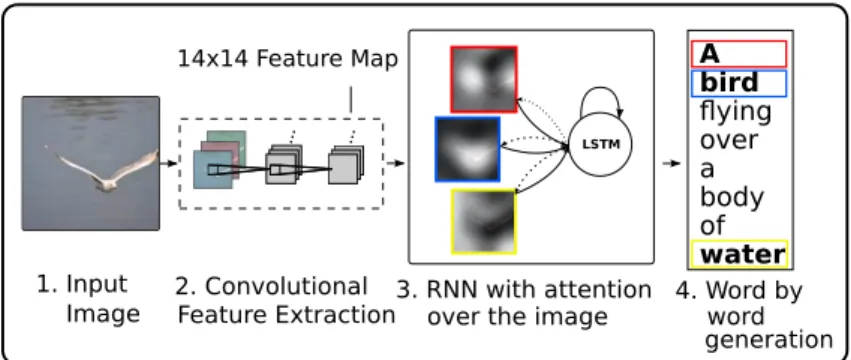
Figure 1.Our model learns a words/image alignment. The visual-ized attentional maps (3) are explained in section3.1&5.4

1. Input

Image 2. ConvolutionalFeature Extraction3. RNN with attention LSTM

4. Word by word 14x14 Feature Map

over the image

generation A bird flying over a body of water

has significantly improved the quality of caption

genera-tion using a combinagenera-tion of convolugenera-tional neural networks

(convnets) to obtain vectorial representation of images and

recurrent neural networks to decode those representations

into natural language sentences (see Sec.

2

).

One of the most curious facets of the human visual

sys-tem is the presence of attention (

Rensink

,

2000

;

Corbetta &

Shulman

,

2002

). Rather than compress an entire image into

a static representation, attention allows for salient features

to dynamically come to the forefront as needed. This is

especially important when there is a lot of clutter in an

im-age. Using representations (such as those from the top layer

of a convnet) that distill information in image down to the

most salient objects is one effective solution that has been

widely adopted in previous work. Unfortunately, this has

one potential drawback of losing information which could

be useful for richer, more descriptive captions. Using more

low-level representation can help preserve this information.

However working with these features necessitates a

power-ful mechanism to steer the model to information important

to the task at hand.

In this paper, we describe approaches to caption

genera-tion that attempt to incorporate a form of attengenera-tion with

arXiv:1502.03044v2 [cs.LG] 11 Feb 2015

Figure 3.3: Show, Attend and Tell model architecture. [57]

Show, Attend and Tell: Neural Image Caption Generation with Visual Atten-tion

Show, Attend and Tell [57] is method, made by researchers from universities in Toronto and Montreal, which introduced an attention based model. Attention is one of the most interesting parts of the human visual system. Rather than compressing an entire image into a static representation, attention allows for salient features to dynamically come to the forefront as needed. Proposed model has encoder-decoder architecture with feedback connections for attention. Overall structure of the model is on Figure 3.3. Encoder part use a CNN to extract set of feature/annotation vectors (not just one). Each of the vectors correspond to a part of image. To obtain a correspondence between them, features from a lower convolutional layer are used.

Decoder part is a LSTM network working of the word level, which generates, apart from the word of the output, a context vector - a dynamic representation of the relevant part of the image at time 𝑡. The paper explored two attention mechanisms computing the context vector from the annotation vectors. First is the stochastic “hard” mechanism, which interprets the values in the context vector as the probability that corresponding location is the right place to focus, while producing the next word. Second is deterministic “soft” mechanism introduced in [2], which gives the relative importance of the location by blending values of all annotation vectors together. This method is fully trainable by the standard SGD methods.

Article also shows how we can gain insight and interpret the results of the model by visualizing where and on what was the attention focused. Examples of the attention visu-alizations with both, correct and wrong generations, are on Figure3.4. Visualizations show that the model can attend even a “non-object” regions. This adds an extra layer of inter-pretability to the output. The model learns alignments that correspond very strongly with human intuition and, even, in the cases of mistakes, we can understand why the captions were generated.

Similarly to previous article, Show, Attend and Tell used VGGnet [47], a CNN trained on the ImageNet, which was not finetuned. Model was trained with several algorithms and researchers found that for Flickr8k dataset, RMSProp worked best, while for Flickr30k and MSCOCO datasets, Adam [34] algorithm was used. Performance during training was also improved by creating minibatches of sentences with same length, which greatly improved convergence speed.

Co rr ec t W ro ng

Figure 3.4: Examples ofShow, Attend and Tell attention. [57]

CNN CNN CNN CNN CNN LSTM LSTM LSTM LSTM LSTM LSTM LSTM LSTM LSTM LSTM W1 W2 W3 W4 WT

Visual Features Sequence Learning Predictions Visual Input

Figure 3.5: TheLRCN model architecture for video processing. [11]

Long-term Recurrent Convolutional Networks for Visual Recognition and De-scription

The research group from Berkeley presented Long-term Recurrent Convolutional Networks

(LRCN) [11], which combines network with convolutional and long-range temporal layers for several tasks. It is possible to apply LRCN to recognize activity performed on the video (sequential input _↦→ fixed output), generate description of the image (fixed input _↦→ sequential output) or describe video (sequential input_↦→ sequential output).

Architecture of the proposed model, see Figure 3.5, is similar to theShow, Attend and Tell, as image is processed by CNN and sent to the input of the LSTM in each time step. Feedback attention connections are missing in this model. According to the task specification, method can use separate convolutional networks, different for each time step with specific input, or single CNN throughout all the time steps.

LRCN tied with Show, Attend and Tell in MS COCO Captioning Challenge for the third place. However, this does not mean the models are equal in general performance, as each of them focuses on different research topic.

3.2

Datasets

Large amounts of data are necessary requirement in training deep neural nets like CNNs and RNNs, as well as sufficient computing power. Access to the machines and hardware suitable for training has been made in recent years extremely easy, with the rise of virtualization services. Obtaining enough data is different issue and it is currently the biggest problem. Especially, creation of image captioning datasets is quite complicated. As there is no automatized way to generate data, all the image descriptions have to be human-generated. This is one of the reasons, only few specialized datasets are created.

There are two main options how to get images and captions. First way is, by using user-generated data from an online service, most commonly Flickr2. However, these captions are not made specifically for the task and could be prone to error. Second option is to gather only images, again from Flickr or other online services, and create captions for direct use in the dataset manually. Amazon Mechanical Turk3 is heavily used for this task.

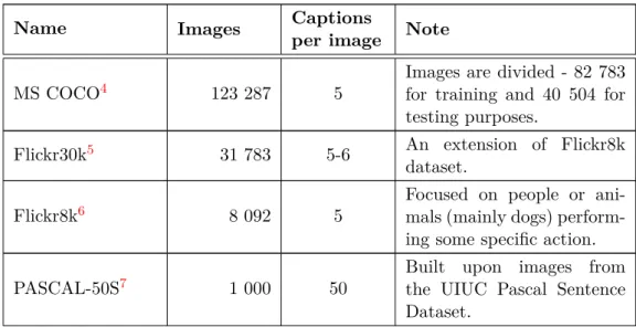
Following Table 3.1 lists the most popular datasets. All these datasets were created directly for the image captioning task, with captions generated through Amazon Mechanical Turk. Flickr8k [25], from 2013, was one of the first datasets created for this purpose. It has been later expanded into Flickr30k [58]. The biggest dataset is Microsoft Common Objects in Context (MS COCO) [6], created for the MS COCO captioning challenge. CIDEr [53] datasets PASCAL-50S, ABSTRACT-50S are youngest mentioned, designed specifically for evaluation with the CIDEr metric discussed in section3.3.

Table 3.1: Image captioning datasets.

Name Images Captions

per image Note

MS COCO4 _{123 287 5}

Images are divided - 82 783 for training and 40 504 for testing purposes.

Flickr30k5 31 783 5-6 An extension of Flickr8k

dataset.

Flickr8k6 _{8 092 5}

Focused on people or ani-mals (mainly dogs) perform-ing some specific action.

PASCAL-50S7 1 000 50

Built upon images from the UIUC Pascal Sentence Dataset.

2_{Flickr is a popular image hosting website and an online community. (https://www.flickr.com)} 3

Amazon Mechanical Turk is crowdsourced Internet marketplace for tasks that computers are currently unable to do. (https://www.mturk.com)

4

MS COCO project: http://mscoco.org/dataset/

5_{Flickr30k project: http://shannon.cs.illinois.edu/DenotationGraph/} 6

Flickr8k project: http://nlp.cs.illinois.edu/HockenmaierGroup/8k-pictures.html

7

Table 3.1: Image captioning datasets.

Name Images Captions

per image Note

ABSTRACT-50S8 500 50

Built upon images from the Abstract Scenes Dataset. No photos.

3.3

Evaluation

Recent progress in fields like machine translation, which are very similar to image cap-tioning, caused spike of interest in evaluating regular text output accuracy. Although, sometimes it is not clear, if a description of an image is the best option available, some degree of assessment is possible. The best results can be obtained by asking live raters to score the usefulness of each description. Subjective scores can vary, but their average over many raters are usually quite accurate. However, this method consumes tremendous amount of time and external raters are necessary in most cases. Like with data generation, tools like Amazon Mechanical Turk are used to great extent, but need for automated tools is evident.

3.3.1 Automated metrics

Assuming that one has access to human-generated captions, which is ground truth in our case, completely automated metrics are available. Even though all of them compute how alike are model descriptions to human-generated, different ratings are used by different metrics and even differences between used settings and implementations of one metric can invalidate the results. This raises the question, how can we compare results of different works, despite them using the “same” evaluation method. Microsoft group of researchers, team responsible for MS COCO, addresses this issue in [6]. They created an evaluation server9, which has many automated metrics, with several configurations, including all men-tioned here. This server should serve as a reference point for comparison of image captioning models.

Among the most popular metrics belong BLEU, METEOR, and CIDEr. The rest of this section is describing and discussing their properties. BLEU (Bilingual Evaluation Under-study) [45] has been the most commonly used metric, which was created in 2002 to evaluate quality of machine translated text. Scores are computed on individual segments, usually sentences. BLEU has high correlation with human judgments and is very popular, even for captioning tasks. However, it is becoming outdated, as according to this metric, automatic methods are now outperforming humans, which is senseless. Four different variations of BLEU are used in MS COCO evaluation server.

METEOR (Metric for Evaluation of Translation with Explicit Ordering) [35] is another metric for the evaluation of machine translation, slightly younger than BLEU, from 2007. Scoring generated translations is performed by aligning them to one or more reference

8

See footnote7.

9

translations. Metric was designed to fix some problems of the BLEU. It can also look for synonyms and perform stemming on input words.

Metric designed directly to caption evaluation – CIDEr (Consensus-based Image De-scription Evaluation) [53] was introduced in 2015. This is still a very new metric, but with growing popularity as it correlate well with human judgment. Main idea of this metric is improving quality of the metric with growing number of captions for the single image. This can be observed on datasets introduced with it (see section3.2).

Chapter 4

Model design

In the previous chapters, the basics of creating neural networks have been laid down, with special focus on RNN units like LSTM and GRU, and CNNs. Chapter 2 also included description of trends in language modeling with RNNs - word and character level models. Following chapter 3 described the current approaches to image captioning and how are state-of-the-art models designed. Chapter also introduced most popular image captioning datasets and evaluation metrics in a short list.

Equipped with the knowledge of previous chapters. In is chapter I will propose the architecture of an image captioning model and describe in detail each part and their con-nections (section4.1). Second part of this chapter (section4.2) is about training procedure of the proposed model - which algorithms and datasets are used, and other details.

4.1

Overall architecture

As a result of the previous research, I designed an image captioning model with the encoder– decoder architecture, slightly based on the Show and Tell [54] and Show, Tell and At-tend [57] models. In this section I describe the CNN encoder part of the model, then, in separate sections 4.1.1 and 4.1.2, RNN modeling language and how to feed the image encoding to the RNN. Throughout the section, all the descriptions refer to the diagram on Figure 4.1, as each of them discuss different parts of the image.

The CNN used in this model is VGGnet [47] - a 16-layer network trained on ImageNet. The same one as the one inFrom Captions to Visual Concepts and Show, Attend and Tell

papers. Input of the CNN is a fixed-size224_×224RGB image, which passes through a stack of convolutional layers with very small receptive fields: 3_×3, and rectifiers. Throughout the network, some of the convolutional layers are followed by max-pooling.

Original network produces a probability distribution over 1000 ImageNet classes. For my purposes, I removed the last softmax layer, as well as last fully-connected layer fc8, which is the approach used by From Captions to Visual Concepts. Thus, output of the CNN has size of 4096, which is then propagated to the rest of the model.

The image encoding produced by CNN has to be preprocessed before entering the RNN. For this purpose, I introduced an “adapter” network, which solves problems with the hidden state initialization algorithm. Both, the adapter and algorithm are described in section 4.1.2.

LSTM <start> T T w w o LSTM LSTM LSTM LSTM LSTM LSTM LSTM LSTM LSTM LSTM LSTM

log p1(S1) log p2(S2) log p3(S3)

S0 S1 S2

Linear Linear Linear

Lin ear Lin ear tan h

Figure 4.1: Architecture of the proposed model.

4.1.1 Language model

Language modeling RNN of this model is based on Section 2.2.2. Captions are generated on character level, without any embeddings. Inputs and outputs of the RNN are the same one-hot encoding. Set of characters, created from the whole training dataset, is completed with two extra special characters <start>and <stop>, which respectively mark beginning and the end of the caption. Since caption can be any sentence, its length is unbounded.

Structure of the recurrent network is sequential and can be considered small in com-parison of other networks commonly used. See Figure 4.1. Core of the network is stack of LSTM layers - experiments were performed on networks with 2 to 5 recurrent layers. Size of LSTMs range from 200 to 500 units per layer, as networks with 150-250 units are able to generate text on character level, without grammatical errors. Size of the network is then increased to accommodate the need to generate correct captions and to distinguish between them. One Linear layer is following LSTMs, transforming the output of the LSTM to the size of the used one-hot encoding. On the very end of the network is a softmax layer, generating the probability distribution of next character in the sequence.

The sequence generation starts by feeding the RNN with<start>symbol. Forward pass through the network is computed and generated character is sampled from the probability distribution. Sampled character is then sent to the network as input in the next time step. This procedure is repeated until the<stop>symbol is sampled from the distribution. 4.1.2 Hidden state initialization

As the both necessary parts, “encoder” and “decoder”, have been described, the way of connecting them is now required. Sending the image encoding to RNN as first input, similarly to Show and Tell [54] is not possible, because character encoding of the caption alters input significantly. Fortunately, LSTMs have a hidden state, a “cell”, which requires initialization. AsShow and Tell[54] demonstrated, showing the image encoding to the RNN at the beginning of caption generation is enough, therefore, initialization of the LSTM’s

hidden state with proper image encoding based vector should suffice.

Hidden state of the LSTM is denoted in Equations (2.3) to (2.8) as vector 𝐶𝑡. As

the sequence processing, starting with input 𝑥1 requires 𝐶0, which has no specific value1,

recurrent layers can be initialized by injecting a new state vector. Vector 𝐶 has a definite size for each LSTM layer, which is equal to the layer size and the output vector. For example, in the LSTM with 200 units, although input vector being unrestrained, output and hidden state vectors size will always be 200. Throughout time, the hidden state usually takes values in range between[−2,2], which align well to initialization around 0.

Output of the CNN is not suitable to be directly inserted to RNN, for several reasons. First, it has a different size(4096), which is much more than necessary for LSTM. Second, CNN uses ReLUs as nonlinearity, which do not produce negative output. This limits the LSTM state space significantly. Both issues are possible to solve by introducing an “adapter” network between the CNN and RNN in the model. The adapter can be very small network, as solving the above mentioned problems is the only task required. In my model, visualized on Figure4.1, I created a network with one linear layer for adjusting size of the output, followed by hyperbolic tangent and second linear layer, which should solve the negative numbers issue.

Last question to cover in the initialization procedure is, how many of the RNN’s stacked LSTM layers will be initialized by the adapter and how many will stay unbounded. Possible solutions can range from initializing only the first recurrent layer to all the recurrent layers in the network, or any count between them. While initializing multiple layers, matter of whether all the layers will have the same input or each of them its own, has to be discussed. As I have not found any adequate solutions and research to this topic, it is covered in Chapter 6, as part of experiments with the model.

4.2

Training

Training is, together with architecture, one of the most important things in deep learning models. Specific training procedure can decide, how fast can model learn the task and whether it can learn the task at all. Proposed image captioning model is relatively simple, from training point of view, as it is end-to-end trainable by standard gradient descent methods. Training will be performed on training part of MS COCO dataset, mentioned in section 3.2, which consists of 82 783 images and 5 captions per image.

Complete procedure is divided into two parts. First part works only with the language model and train the LSTM layers to produce proper English words and sentences. In the second stage, the encoder part of network - CNN and adapter, is connected to the model and adds more constraints to the caption generation. Both training stages have appropriate sections in the following text, describing them more thoroughly.

Pretraining RNN

As mentioned earlier, it is useful to train the language model, to the point it can gener-ate English words and sequences, because words are often repegener-ated across captions and sentences generally have the same structure. This can be seen in the training dataset, as it contains only 25 000 different words. Pretraining the RNN speed up the training and we can also verify RNN trained properly before connecting it with the other parts of the model.

1

Loss function used in this work is the sum of the negative log likelihood of the character at each step as follows:

𝐿(𝑆) = ₋

𝑁

∑︁

𝑡=1

𝑙𝑜𝑔 𝑝𝑡(𝑆𝑡). (4.1)

During pretraining, the above loss is minimized with respect to all the parameters of the RNN. Method used to minimize this loss is Adam [34], with parameters 𝛽1 = 0.92, 𝛽2 =

0.999, and learning rate 𝛼= 0.001. Training used minibatches of size 15, which is number selected mostly for implementation reasons further discussed in chapter 5.

Full model training

With the language model trained to generate random sentences, it is very easy to connect the rest of the model to it to perform full model training. Most of the information described in this part is same to the pretraining, for example, loss function is virtually the same negative log likelihood: 𝐿(𝐼, 𝑆) = ₋ 𝑁 ∑︁ 𝑡=1 𝑙𝑜𝑔 𝑝𝑡(𝑆𝑡). (4.2)

However, the loss is minimized with respect to all the parameters of RNN as well as the

adapter and CNN. Gradients propagated to the initial state of RNN are copied to the other part of the network. Each part (CNN, adapter, RNN) has its own instance of gradient descent algorithm, however, Adam [34], with same parameters 𝛽1 = 0.92, 𝛽2 = 0.999, and

learning rate𝛼 = 0.001is used for all three options. Minibatch size 15 was used.

During full model training, finetuning of CNN is optional. Finetuning can provide some improvements in results, but it also greatly expands the number of training parameters. Not training CNN increase training speed and allows easier localization of potential mistakes related to input of theadapter or RNN.

Inference

There are multiple approaches that can be