Comparing Distribution and Quantile Regression

(1)

IEF

EIEF Working Paper 15/11

October 2015

Comparing Distribution

and

Quantile Regression

by

Samantha Leorato

(University of Rome “Tor Vergata”)

Franco Peracchi

(Georgetown University, University of Rome

“Tor Vergata” and EIEF)

EIEF WORKING PAPER s

ERIE

s

(2)

Comparing Distribution and Quantile Regression

∗

Samantha Leorato

Department of Economics and Finance, University of Rome Tor Vergata

Franco Peracchi

Department of Economics, Georgetown University

Department of Economics and Finance, University of Rome Tor Vergata

Einaudi Institute for Economics and Finance

October 21, 2015

Abstract

We study the sampling properties of two alternative approaches to estimating the conditional distri-bution of a continuous outcomeY given a vectorX of regressors. One approach – distribution re-gression – is based on direct estimation of the conditional distribution function; the other approach – quantile regression – is instead based on direct estimation of the conditional quantile function. Indirect estimates of the conditional quantile function and the conditional distribution function may then be obtained by inverting the direct estimates obtained from either approach or, to guarantee monotonicity, their rearranged versions. We provide a systematic comparison of the asymptotic and finite sample performance of monotonic estimators obtained from the two approaches, considering both cases when the underlying linear-in-parameter models are correctly specified and several types of model misspecification of considerable practical relevance.

KEYWORDS: Distribution regression; quantile regression; linear location model; nonseparable models.

JELCLASSIFICATIONS: C1, C21, C25.

∗ _{We thank the Editor and three anonymous referees for their comments. We also thank Jana Jureˇcková, Blaise Melly,}

Frank Vella, and especially Roger Koenker for useful discussions. Corresponding author: Samantha Leorato ([email protected]).

(3)

1

Introduction

In this paper we compare the sampling properties of two alternative approaches to estimating the con-ditional distribution of a continuous outcomeY given a vectorX of regressors.

One approach – the distribution regression or DR approach – models parametrically the conditional distribution function (CDF)F(y_|x) =Pr_{Y _≤y_|X =x_}locally in y_{∈ Y}, and obtains estimates ˆF(_{· |}x) of the CDF by fitting a sequence of binary regression models at a finite number of cutoff values y1, . . . ,yJ,

each model corresponding to the conditional mean of the binary indicator D_j =1{Y ≤ y_j}. In fact, a convenient strategy is to model notF(y|x)directly, but rather the conditional log-odds function (CLF) t(y|x) =lnF(y|x)−ln 1₋F(y|x). While this strategy leaves the range oftcompletely unrestricted, it guarantees that estimates ofF(y_|x)obtained by inverting estimates oft(y_|x)are bounded between zero and one. An important special case is the linear-in-parameters specificationt(y|x) =P(x)>θ(y), where P(x) is a vector of known transformations of the regressors, θ(y) is a point in some finite-dimensional parameter space and all elements ofθ may vary with y. Although restrictive, this spec-ification leads to models that are easy to estimate and to interpret. Further, any smooth CLF can be approximated arbitrarily well by one that is linear in parameters. This approach, first proposed by Foresi and Peracchi (1995), has recently been considered by Fortin, Lemieux and Firpo (2011), Rothe (2012), Chernozhukov, Fernández-Val and Melly (2013) and Hothorn, Kneib and Bühlmann (2014).

The other approach – the quantile regression or QR approach – models parametrically the condi-tional quantile function (CQF)Q(p|x) = inf_{y ∈ Y: F(y|x) ≥ p}locally in p ∈(0, 1), and obtains estimates of the CQF by fitting a sequence of asymmetric least absolute deviation regressions at a finite number of quantile levels p1, . . . ,pJ. Here again, an important special case is the linear-in-parameter

specification Q(p|x) = P(x)>γ(p), where P(x) is a vector of known transformations of the regres-sors, γ(p) is a point in some finite-dimensional parameter space and all elements ofγmay vary with p. This approach, first proposed by Koenker and Bassett (1978), has been generalized in many direc-tions, including penalized likelihood methods, semi-parametric methods, methods for nonidentically distributed or dependent observations, extremal quantile regression, and weighted quantile regression (see Koenker 2005 for a review).

The CDF and the CQF are equivalent characterizations of the conditional distribution ofY givenX, as they are generalized inverses of each other, that is,Q(F(y|x)|x) ≤ y and F(Q(p|x))≥ p, which implies thatF(y|x)≥pif and only ifQ(p|x)≥ y. Thus, by analogy with this relationship, given a direct estimate ˆF(· |x)of the CDF, one may obtain an indirect estimate of the CQF by taking its generalized inverse ˜Q(p|x) =infy: ˆF(y|x)≥p . Similarly, given a direct estimate ˆQ(· |x)of the CQF, one may

(4)

obtain an indirect estimate of the CDF by taking its generalized inverse ˜F(y_|x) =infp: ˆQ(p_|x)_≥ y . In the unconditional case, where no parametric assumption is needed, the empirical distribution function and the empirical quantile function are generalized inverses of each other, so the DR and QR approaches are equivalent. When conditioning on a set of regressors, however, the DR and QR approaches are generally not equivalent because a convenient parametric model for the CQF, such as a linear-in-parameter specification, need not imply an equally convenient or easily interpretable model for the CDF, and viceversa.

Further, estimates based on linear-in-parameter specifications, while easy to obtain, need not be proper since they need not satisfy the key monotonicity properties of the CDF and the CQF, namely F(y0|x) ≥ F(y|x) whenever y0 > y and Q(p0|x) ≥ Q(p|x) whenever p0 > p, for any x. Non-monotonicity of the estimates may just be a finite-sample problem or may reflect, more fundamentally, misspecification of the underlying parametric model for the CDF or the CQF. In any case, far from being a minor technical problem, the issue of how to guarantee monotonicity is of central importance, as in-direct estimates can only be proper if they are obtained by inverting a proper estimate of the CDF or the CQF, and only in this case their asymptotic properties can be derived by means of the functional delta method.

Among the various ways of guaranteeing monotonicity proposed in the literature, in this paper we concentrate on the rearrangement procedure suggested by Chernozhukov, Fernández-Val and Galichon (2010), which is particularly attractive for its general nature and computational simplicity. We provide a systematic study of the asymptotic and finite sample performance of monotonic estimators obtained from the DR and QR approaches, considering both cases when the underlying linear-in-parameter mod-els are correctly specified and several types of model misspecification of considerable practical rele-vance. We focus on bias, precision (as measured by the variance) and efficiency (as measured by the mean squared error) of the various estimators, both in finite samples and asymptotically. Of course, efficiency is only one of the many theoretical and practical criteria for comparing estimators, and other criteria may be taken into account, such as statistical robustness, computational ease, etc.

We assume throughout the paper that the available data _{(Xi,Yi)}ni=1 are a sample from the joint

distribution of the random vector(X,Y)with supportX × Y, whereX ⊆RkandY ⊆R. This restric-tive assumption helps simplify the presentation, but our results can easily be generalized to the case of heterogeneous or dependent observations. We also assume that the distribution of X has a finite nonsingular second moment matrix and that, for any x ∈ X, the CDF ofY given X = x is continuous and strictly increasing, which implies that the conditional density f(y|x)ofY givenX =x exists and

(5)

is finite and bounded away from zero. This in turn implies that the CDF and the CQF are inverses of each other, that is, F(Q(p|x)|x) = p andQ(F(y|x)|x) = y. We further assume that our linear-in-parameter models for the CDF and the CQF always include an intercept, and to simplify notation we setP(X) = (1,X>)>≡X andP(x) = (1,x>)>≡x. Finally, we denote byl∞(S)the space of bounded and measurable real-valued functions defined onS.

The remainder of the paper is organized as follows. Section 2 introduces the direct DR estimator of the CDF and the indirect estimator obtained by rearrangement. Section 3 introduces the direct QR estimator of the CQF and the indirect estimator obtained by rearrangement. Section 4 compares the asymptotic properties of estimators obtained under the DR and the QR approach, both when the linear-in-parameter models on which they are based are correctly specified and when they are not. Section 5 compares the finite sample properties of the various estimators considered via a set of Monte Carlo experiments. Finally, Section 6 summarizes and offers some conclusions.

2

DR estimators

Given a random sample_{(Xi,Yi)}n_i₌1 from the distribution of(X,Y) and a linear-in-parameter model

t(y_|x) = x>θ(y) for the CLF, an estimate θˆ_n(y) ofθ(y) may be obtained by maximizing over the parameter space the average pseudo log-likelihood

L_n(θ;y) =n−1 n X i=1 D_{y i}X>_i θ₋ln 1+expX>_i θ,

where D_{y i}=1{Y_i≤ y}. Givenθˆ_n(y), the direct DR estimate of the population CDF at the cutoff value y is ˆF_n‡(y_|x) =Λx>θˆ_n(y), where Λ(u) =eu/(1+eu)is the standard logistic distribution function with densityλ(u) =Λ(u)(1₋Λ(u)).

The population analog of ˆF_n‡(y|x)is denoted byF‡(y|x) =Λ x>θ(y), whereθ(y)maximizes the expected pseudo log-likelihood L(θ;y) =EDyX>θ−ln 1+exp(X>θ)

over the parameter space. If the assumed model for the CLF is correctly specified, thenF‡(y|x) =F(y|x)for almost all x and y values, so a consistent indirect estimator of the CQF may simply be obtained by taking the generalized inverse of ˆF_n‡. However, if the assumed model is misspecified, then ˆF_n‡converges to a limit functionF‡ that differs from F on a subset ofX × Y with positive measure. This has two consequences. First, the direct estimator ˆF_n‡ is inconsistent for F, so the indirect estimator obtained by taking the generalized inverse of ˆF_n‡is inconsistent forQ. Second, although bounded between zero and one, the limit function F‡need not be a proper CDF because it need not be nondecreasing in y for all x. This implies that the

(6)

generalized inverse of F‡ is not a continuous function, which prevents one from using the functional delta method to study the asymptotic properties of the CQF estimator obtained by inverting ˆF_n‡.

A simple way to guarantee monotonicity is the rearrangement procedure proposed by Chernozhukov, Fernández-Val and Galichon (2010).1 Their procedure relies on the fact that, even when ˆF_n‡is nonmono-tonic, a proper estimate of the CDF is ˆF_n+(y|x) =inf{p: ˆQ+_n(p|x)≥p}, where

ˆ Q+_n(p_|x) = Z ∞ 0 1{Fˆ_n‡(y_|x)_≤p_}d y₋ Z 0 −∞ 1{Fˆ_n‡(y_|x)>p_}d y (1) can be shown to be a proper estimate of the CQF (the proof is in Chernozhukov, Fernández-Val and Galichon 2007). Notice that while the DR approach does not directly estimate the CQF, rearrangement produces joint estimates of both the CDF and the CQF. If ˆF_n‡ is monotone, then ˆF_n+ and ˆF_n‡coincide. In general, ˆF_n+(y|x) =Fˆ_n‡(y|x)at all points where ˆF_n‡(y|x)is increasing in yand the equation ˆF_n‡(y|x) = phas a unique solution. The same rearrangement procedures applied to the limit functionF‡gives both its rearranged version ofF+ and its generalized inverseQ+.

Rearrangement offers two main advantages. First, the rearranged estimator ˆF_n+ is the continuous and Hadamard differentiable inverse of ˆQ+_n, so its asymptotic properties can be derived via the functional delta method. Second, as shown by Chernozhukov, Fernández-Val and Galichon (2010) in their Monte Carlo experiments, ˆF_n+ has a smaller bias than the original estimator ˆF_n‡.

Chernozhukov, Fernández-Val and Melly (2013) derive the asymptotic properties (as n_{→ ∞}) of the stochastic processespnθˆn(y)−θ(y)

,pn Fˆ_n‡(y|x)−F‡(y|x)andpn Fˆ_n+(y|x)−F+(y|x). Their results, summarized in Theorem 1 below for the case when the assumed model is linear in pa-rameters, rely on the following two assumptions:

A.1: There exist y < y in the interior of _Y such that, for any y _∈[y,y], θ(y) uniquely maximizes L(θ;y)on a compact subsetΘof the parameter space.

A.2: For any x∈ X, the number of critical points_{y:∂_yF‡(y|x) =0_}is finite.

Assumption A.1 and the assumption thatX has finite nonsingular second moments guarantee that Ln(θ;y)is twice differentiable inθ and that its first and second partial derivatives have finite second

moments. It also implies that the matrixH(y) =Eλ X>θ(y)X X>is finite and negative definitive for all y∈[y,y], and thatθ(y)is continuously differentiable iny. In fact, applying the implicit function theorem to the system of equations∂L(θ;y)/∂θ=0 shows thatθ(y)is continuous and differentiable 1_{Other procedures that guarantee monotonicity have been proposed by Foresi and Peracchi (1996), Hall, Wolff and Yao}

(7)

in y, with derivativeθ0(y) = [H(y)]−1 Ef(y|X)X, so it is also continuously differentiable in y. As a consequence,F‡(y|x)is continuously differentiable in both its arguments.

Assumption A.2 guarantees that, for all x, y andp, the equation F‡(y|x) =p, or equivalently the equationx>θ(y) =ln[p/(1₋p)], has a finite numberN(p|x)of roots which we denote by yj(p|x).

We also denote byU_x∗⊂(0, 1)the set of regular values of the functionF‡(y|x), that is, the subset of the codomain of F‡(_{· |}x) whose preimage does not contain critical points, and define (0, 1)_X∗ = {(p,x):p∈ Ux∗,x ∈ X }.

Theorem 1 If A.1 holds, then the processθˆ_n(·)is uniformly consistent forθ(·), that is,sup_y_≤_y_≤_ykθˆn(y)−

θ(y)k = op(1), and the process H(·)

p

nθˆn(·)−θ(·)

converges weakly on l∞([y,y])to a zero-mean multivariate Gaussian process B_D(·)with covariance function

ΣD(y,y0) =E Dy−Λ(X>θ(y)) Dy0−Λ(X>θ(y0)) X X>, y ≤ y0.

In addition, for any compact subsetK ⊂ [y,y]× X, the processpn Fˆ_n‡(y|x)−F‡(y|x), indexed by

(y,x), converges weakly on l∞(K)to a zero-mean Gaussian process W defined as

W(y|x) =λ x>θ(y)x>H(y)−1BD(y). (2)

If A.1–A.2 hold then, for any compact subsetK ⊂(0, 1)_X∗, the processpn Qˆ+_n(p|x)−Q+(p|x), indexed by(p,x), converges weakly on l∞(K)to a zero-mean Gaussian process C_W defined as

C_W(p|x) =− N(p|x) X j=1 W(y_j(p|x)|x) ∂_yF‡(y_j(p|x)|x) .

Finally, lettingK∗=¦(y,x)∈[y,y]× X: F+(y|x),x∈ K©, the processpn Fˆ_n+(y|x)−F+(y|x), indexed by(y,x), converges weakly on l∞(K∗)to a zero-mean Gaussian process DW defined as

D_W(y|x) =−   N(F‡(y|x)|x) X j=1 1 ∂_yF‡ y_j(F+(y|x)|x) x   −1 C_W F+(y|x) x .

The function C_W(p_|x) in Theorem 1 is the Hadamard differential ofQ+ at W tangentially to the space of continuous functions defined on_{Y X} =(y,x): F+(y|x),x∈(0, 1)_X∗ (see e.g. van der Waart 1998). If F‡ is strictly increasing in y then the equation F‡(y|x) = p has a unique root and F+(y_|x) = F‡(y_|x) for all x, y and p, soC_W(p_|x) = ₋W Q+(p_|x)x

/∂yF‡ Q+(p|x) x and DW(y|x) =W(y|x).

(8)

It follows from Theorem 1 that the asymptotic variance of ˆF_n‡(p_|x) is equal to V Fˆ_n‡(p|x) = λ x>θ(y)2 x>VD(y)x, whereVD(y) =H(y)−1ΣD(y,y)H(y)−1 denotes the asymptotic variance of

ˆ

θn(y). If the assumed linear-in-parameter model for the CLF is correctly specified, then ΣD(y,y) =

H(y)andVD(y) =H(y)−1, so the asymptotic variance of ˆFn‡(y|x)simplifies toV Fˆ

‡

n(y|x)

=λ x>θ(y)2 x>H(y)−1x.

3

QR estimators

An alternative to directly estimate the CDF is to first estimate the CQF and then obtain indirect estimates of the CDF by taking the generalized inverse or by rearrangement. To fix the ideas, consider the linear location model

Y =α+X>β+U, (3)

whereU is a random error distributed independently ofXwith a strictly increasing distribution function G. Its CQF isQ(p_|x) =x>γ(p), whereγ(p) = α+G−1(p),β>>. This model has the restrictive feature that Q(p|x)−Q(p0|x) = G−1(p)−G−1(p0), that is, conditional quantiles corresponding to different values ofpare at a constant distance from each other. A straightforward generalization retains linearity in the parameters but allows all elements ofγ(p) to depend on p, leading to the linear-in-parameter specificationQ(p|x) =x>γ(p), whereγ(p)is a point in some finite-dimensional parameter space and all elements ofγmay vary withp.

Given a random sample_{(Xi,Yi)}ni=1from the distribution of(X,Y)and a linear-in-parameter model

for the CQF, an estimateγˆ_n(p) ofγ(p) may be obtained by minimizing over the parameter space the objective function `n(γ;p) =n−1 n X i=1 ρp Yi−X>i γ ,

whereρ_p(u) =u[p−1{u≤0}]is the asymmetric absolute loss function. Given γˆ_n(p), the direct QR estimate of the population CQF at the quantile levelpis ˆQ∗_n(p|x) =x>γˆ_n(p).

The population analog of ˆQ∗_n(p|x)is denoted byQ∗(p|x) =x>γ(p), whereγ(p)is the minimizer over the parameter space of`(γ;p) =Eρp Y −X>γ

, the population analog of`_n(γ;p). If the assumed model for the CQF is correctly specified, thenQ∗(y|x) =Q(p|x) for almost all x and p values, so a consistent indirect estimator of the CDF may simply be obtained by taking the generalized inverse of ˆQ∗_n. However, if the assumed model is misspecified, then ˆQ∗_nconverges to a limit functionQ∗that differs from Qon a subset of_{Y ×X} with positive measure. This poses the same problems discussed in Section 2. As suggested by Chernozhukov, Fernández-Val and Galichon (2010), a possible solution is again rearrange-ment. When ˆQ∗_n is nonmonotonic, a proper estimate of the CQF is ˆQ◦_n(p|x) = inf_{y: ˆF_n◦(y|x) ≥ p},

(9)

where ˆ F_n◦(y|x) = Z 1 0 1{Qˆ∗_n(p|x)≤ y}d p (4) is a proper estimate of the CDF. The same rearrangement procedures applied to the limit functionQ∗ gives both its rearranged versionQ◦and its generalized inverseF◦. Notice thatQ∗andQ◦coincide ifQ∗ is monotone. Moreover,Q◦(p|x) =Q∗(p|x)provided thatQ∗(p|x)is increasing atpandQ∗(p|x) =p has a unique solution for y=Q◦(p|x).

Chernozhukov, Fernández-Val and Melly (2013)) also provide the QR counterpart of Theorem 1. Their results, summarized in Theorem 2 below, rely on the following two assumptions:

B.1: There existp <p in the interior of(0, 1)such that, for any p∈[p,p],γ(p)uniquely minimizes `(γ;p)on a compact subsetΓ of the parameter space.

B.2: For any x _{∈ X}, the number of critical points_{p:∂_pQ∗(p_|x) =0_}is finite.

Assumptions B.1–B. 2 play the same role as Assumptions A.1–A.2 in Section 2. In particular, As-sumption B.1 implies that the matrixJ(p) =Ef X>γ(p)|XX X>is finite and positive definite for allpin the closed interval[p,p], and that the functionγ(p)is continuously differentiable on[p,p]with derivativeγ0(p), while Assumption B.2 guarantees that, for allx, y andp, the equationQ∗(p|x) = y, or equivalently the equation x>γ(p) = y, has a finite number N(y_|x)of roots which we denote by pj(y|x). We also denote byYx∗the subset of the codomain ofQ∗(· |x)whose preimage does not

con-tain critical points. Thus,∂_pQ∗(p|x)6=0 for allpsuch thatQ∗(p|x)∈ Y_x∗.

Theorem 2 If B.1 holds, then the processˆγ_n(_·)is uniformly consistent forγ(·), that is,sup_p_≤_p_≤_p_kγˆ_n(p)−

γ(p)k=o_p(1), and the process J(·)pn γˆ_n(_·)₋γ(_·)converges weakly on l∞([p,p])to a zero-mean mul-tivariate Gaussian process BQ(·)with covariance function

ΣQ(p,p0) =E

p−1{Y <X>γ(p)} p0−1{Y <X>γ(p0)}X X>, p≤p0.

In addition, for any compact subset H ⊂[p,p]× X, the processpn Qˆ∗_n(p|x)−Q∗(p|x), indexed by

(p,x), converges weakly on l∞(H)to the zero-mean Gaussian process Z defined as Z(p|x) =x>J(p)−1B_Q(p).

If B.1–B.2 hold then, for any compact subsetK ⊂(0, 1)X∗, the processpn Qˆ+_n(p|x)−Q+(p|x), indexed by(p,x), converges weakly on l∞(_K)to a zero-mean Gaussian process C_W defined as

CZ(y|x) =− N(y|x) X j=1 Z pj(y|x)|x ∂_pQ∗ p_j(y|x)|x .

(10)

Finally, lettingK∗=¦(y,x)∈[y,y]× X: F+(y|x),x∈ K©, the processpn Fˆ_n+(y|x)−F+(y|x), indexed by(y,x), converges weakly on l∞(K∗)to a zero-mean Gaussian process D_W defined as

DZ(p|x) = N(y|x) X j=1 1 ∂_pQ∗ p_j(y|x)|x !−1 CZ(y|x) y=Q◦₍_p_|_x₎ .

The function CZ(p|x) in Theorem 2 is the Hadamard differential of F◦ at Z tangentially to the

andDZ(p|x) =Z(p|x).

It follows from Theorem 2 that the asymptotic variance of ˆQ∗_n(p|x)isV Qˆ∗_n(p|x)

= x>V_Q(p)x, where VQ(p) =J(p)−1ΣQ(p,p)J(p)−1 denotes the asymptotic variance ofγ(p). If the assumed

linear-in-parameter model is correctly specified, thenJ(p) =Ef X>γ(p)|XX X>. In particular, under the linear location model (3),Σ_Q(p,p) =p(1₋p)P_X andJ(p) = g_pP_X, with g_p =g(G−1(p))and g=G0, so the asymptotic variance ofγ(p)simplifies toVQ(p) = [p(1−p)/gp2]P−

1

X .

4

Asymptotic relationships

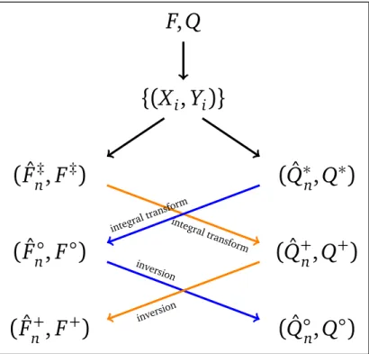
In this section we compare the asymptotic properties of estimators obtained under the two approaches, both when the assumed linear-in-parameter models for the CLF and the CQF are correctly specified and when they are not. Figure 1 summarizes the relationships between the various estimators considered and their population counterparts.

4.1

Correct specification

If the assumed linear-in-parameter models for the CDF and the CQF are both correctly specified, which is essentially equivalent to assuming that the data satisfy the linear location model (3) with logistic errors, then Theorems 1 and 2 imply that, for anyx and all y ∈[y,y] such thatp≤F(y|x)≤ p, the asymptotic variances of all estimators considered are linked by the following relationships

(11)

This set of results implies that, for anyx and allp_∈[p,p]andy _∈[y,y]such thatF(y_|x) =pand Q(p|x) = y, we have

ARE Fˆ_n◦(y|x), ˆF_n+(y|x)=ARE Qˆ◦_n(p|x), ˆQ+_n(p|x).

Thus, the relative performance of the DR and QR approaches in estimating the CDF is asymptotically the same as their relative performance in estimating the CQF. Consistently with this result, Azzalini (1981) found that the approximate mean squared error (MSE) of the direct kernel estimator ˆF of a distribution function (obtained by integrating a kernel density estimator) relative to the MSE of the empirical distribution function is about the same as the MSE of the indirect estimator of the quantile function, obtained by inverting ˆF, relative to the MSE of the sample quantile function.

4.2

Misspecification

If the assumed linear-in-parameter model for the CLF is misspecified, then the DR approach leads to inconsistent estimates, as F‡ no longer coincides with the true CDF. The same is true for the QR ap-proach if the assumed linear-in-parameter model for the conditional CQF is misspecified. In these cases, asymptotic comparison of the various estimators may be based on their MSE, which is asymptotically dominated by bias.

In this section we focus on a fairly general type of misspecification, namely the case when the assumed models for the CLF and the CQF are linear in parameters but the sample observations are generated from the nonseparable data generating process (DGP)

Y =α+X>β+ψ_δ(X,U), (5) whereU is distributed independently ofX as standard logistic,δis a scalar parameter, andψ_δ(X,U)is a term that captures the particular way in which the logistic linear location model may be misspecified. We assume that the function ψ_δ(x,u)varies smoothly with δ for all x andu, and thatψ_δ(x,u) =u only whenδ=0. Thus, whenδ=0, model (5) reduces to the logistic linear location model, in which case our linear-in-parameter models for the CLF and the CQF are both correct.2

The DGP (5) is quite general and encompasses several important types of departure from the logistic linear location model. Notice that the degree to which the logistic linear location model is misspecified 2_{Notice that we are assuming that the DGP is the same for all observations. An alternative is to allow a fraction}_δ_of

the observations to deviate from the assumed model. Asymptotic results for this case are presented in Leorato and Peracchi (2015).

(12)

only depends on the value of the scalar parameterδ, which we will term the “degree of misspecifica-tion”. Whenδ= 0 there is no misspecification, but the precise meaning ofδdepends on the type of misspecification considered.

Under the assumption that the function ψ_δ(x,u) is strictly increasing in u for all x andδ, with inverse functionϕ_δ(x,u), the CDF implied by (5) is

F_δ(y|x) =Λ ϕ_δ(x,y−α−x>β), while its CQF is

Q_δ(p|x) =α+x>β+ψ_δ x,Λ−1(p),

whereΛ−1(p) =ln[p/(1₋p)]. Puttingδ=0 gives the CDF and the CQF of the logistic linear location model, namelyF0(y|x) =Λ y−α−x>β

andQ0(p|x) =α+x>β+Λ−1(p).

The remainder of this section discusses in more detail four types of departure from the logistic linear location model that are of considerable practical relevance and represent the main focus of the Monte Carlo study described in Section 5.

(i) Omitted variables: The GDP takes the following form

Y =α+X>β+δφ(X) +U,

soψ_δ(x,u) =δφ(x) +uandϕ_δ(x,u) =u−δφ(x). By suitable definingX and the functionφ(x), this formulation includes both the case of omitted variables and the case of nonlinearity of the conditional mean ofY.

(ii) Heteroskedasticity: The GDP takes the following form Y =α+X>β+σ_δ(X)U,

whereσ_δ(x) =1+δφ(x)is a positive scale function, soψ_δ(x,u) =σ_δ(x)uandϕ_δ(x,u) =u/σ_δ(x). By suitable definingX and the functionφ(x), this formulation also includes the case when the conditional mean and the conditional variance ofY depend on different sets of regressors.

(iii) Nonlogistic models: The GDP takes the following form Y =α+X>β+G_δ−1(Λ(U)),

where G_δ is a strictly increasing distribution function such thatG0=Λ, soψδ(x,u) =G−δ1(Λ(u))and

(13)

(iv) Transformation models: The GDP takes the following form φδ(Y) =α+X>β+U,

where φ0(y) = y andφδ(y)is strictly monotone in y for everyδ with inverse functionφ_δ−1. In this

caseψ_δ(x,u) =φ−_δ1(α+x>β+u)₋α₋x>β andϕ_δ(x,u) =φ_δ(α+x>β+u)₋α₋x>β. A leading example is when Y is a nonnegative random variable and φ_δ(Y) = Y(1−δ)+1, where Y(1−δ) is the Box-Cox transform ofY, that is,Y(1−δ)= (Y1−δ₋1)/(1₋δ)ifδ₆=1 andY(1−δ)=lnY ifδ=1.3

If we increase the sample size keeping fixed the degree of misspecification δ, then we eventually reach a situation where the bias completely dominates the MSE. The usual approach in order to strike a balance between asymptotic precision and bias is to allow the standard error of estimation and the degree of misspecification to vanish asymptotically at the same rate. Following this approach, Leorato and Peracchi (2015) derive the bias of estimators based on linear models for the CLF or the CQF when the logistic linear location model is locally misspecified, that is, the DGP is of the form (5) butδ=c/n−1/2for some constantc. Their results require two conditions: the functionψ_δ(x,u)must be strictly increasing and differentiable inufor all x andδ, and the function

Ψ(x,u) =lim

δ→0

ψ_δ(x,u)−u δ

must exist and be square integrable inx, uniformly inu. Since all types of misspecification considered in this paper satisfy these two conditions, we can use their results to compute the local asymptotic bias of all our estimators, namely their asymptotic bias under local misspecification.

When δ= c/pn, it follows from Corollary 1 in Leorato and Peracchi (2015) that, for any x ∈ X and all y ∈[y,y], the direct DR estimator ˆF_n‡ of the CDF has the same local asymptotic bias as the rearranged DR estimator ˆF_n+, namely

B Fˆ_n+(y|x)=cλy(x) Ψy(x)−x> Eλy(X)X X> −1 Eλy(X)Ψy(X)X , (6) whereλ_y(x) =λ(y−α−x>β), Ψ_y(x) =Ψ(x,y−α−x>β), λ_y(X) =λ(y−α−X>β)andΨ_y(X) =

Ψ(X,y−α−X>β). Similarly, for anyx∈ X and allp∈[p,p], the local asymptotic bias of the rearranged DR estimator ˆQ+_n of the CQF is B Qˆ+_n(p|x)=−c Ψy(p|x)(x)−x> Eλy(p|x)(X)X X> −1 Eλy(p|x)(X)Ψy(p|x)(X)X , (7) 3_{This particular specification of the Box-Cox transformation model guarantees that (3) holds when}_δ₌_0.

(14)

where y(p_|x) =α+Λ−1(p) +x>β, Ψ_y₍_p_|_x₎(x) =Ψ(x,Λ−1(p)), λ_y₍_p_|_x₎(X) =λ(Λ−1(p) + (x₋X)>β), andΨ_y₍_p_|_x₎(X) =Ψ(X,Λ−1(p) + (x−X)>β). Further, for any x ∈ X and all p∈[p,p], the direct QR estimator ˆQ∗_n of the CQF has the same local asymptotic bias as the rearranged QR estimator ˆQ◦_n, namely

B Qˆ◦_n(p|x)=−cΨy(p|x)(x)−x>(EX X>)−1 Ψy(p|X)(X)X

, (8)

whereΨ_y₍_p_|_X₎(X) =Ψ(X,Λ−1(p)). Finally, for any x ∈ X and all y ∈[y,y], the local asymptotic bias of the rearranged QR estimator ˆF_n◦of the CDF is

B Fˆ_n◦(y|x)=cλy(x)

Ψy(x)−x>(EX X>)−1 EΨ(X,y−α−x>β)X

. (9)

Given these results and Theorems 1–2, we compute the local asymptotic MSE of each estimator as the sum of its asymptotic variance and its local asymptotic squared bias.

Notice that the term in square brackets in (8) is the error in approximating Ψ_y₍_p_|_x₎(x) using the linear least-squares projection ofΨ_y₍_p_|_X₎(X) on X, while the corresponding term in (7) is the error in approximating Ψ_y₍_p_|_x₎(x) using the weighted linear least-squares projection of Ψ_y₍_p_|_x₎(X) on X with weights equal toλ_y₍_p_|_x₎(X). The term in square brackets in (9) is instead the error in approximating

Ψy(x)using the linear least-squares projection ofΨ(X,y−α−x>β)onX, while the corresponding term

in (6) is the error in approximatingΨ_y(x)using the weighted linear least-squares projection ofΨ_y(X) onX with weights equal toλ_y(X).

As shown in the Appendix, the local asymptotic bias of the various estimators depends on the prop-erties of the function Ψ(x,u). In the case of omitted variables, where Ψ depends only on x, all esti-mators are generally inconsistent, but the asymptotic bias of ˆQ◦_n does not depend on p. In the case of heteroskedasticity, again all estimators are generally inconsistent, but the asymptotic bias of ˆQ◦_n is pro-portional toΛ−1(p), so it vanishes whenp=1/2. In the case of nonlogistic models,Ψdepends only on u, sayΨ(x,u) =ζ(u)for some functionζ, so the asymptotic biases of ˆF_n◦and ˆQ◦_nare both proportional to

x>P_X−1(EX)−1. Sincex>P_X−1(EX) =1 for anyx, the QR estimators have no asymptotic bias. The situ-ation is just the opposite for transformsitu-ation models. In this caseΨ(x,u) =χ(α+x>β+u)for some func-tionχ, so the bias of ˆF_n+is proportional to x>H(y)−1Eλy(X)X

−1, whereH(y) =Eλy(X)X X>

. Sincex>H(y)−1E[λy(X)X] =1 for anyx and y, ˆFn+has no asymptotic bias. A similar argument holds

for ˆQ+_n. Thus, the DR estimators have no asymptotic bias.

By combining two or more sources of misspecification, the four types of departures from the logistic linear location model considered in this section can be used to construct more complex scenarios.4

4_{For example, in the case of a Box-Cox transformation model, a logistic error distribution is generally misspecified because}

it is unbounded from below: the combination in this case of the two forms of misspecification (iii) and (iv) produces a function of the formΦ(x,u) =ζ(u)χ(α+x>_β₊_u₎_{, and both approaches lead to inconsistent estimates.}

(15)

5

Finite-sample properties

In this section we present the results of a set of Monte Carlo experiments aimed at comparing the finite-sample properties of DR and QR estimators based on simple linear-in-parameter models for the CLF and the CQF.

5.1

Monte Carlo design

We compute DR and QR estimators from samples of sizengenerated from a DGP of the form (5), where X is a single regressor uniformly distributed on the interval(0, 1),U has a standard logistic distribution, the functionψ_δ(x,u)varies smoothly withδfor all x andu, is strictly increasing inufor all x andδ, and is such thatψ_δ(x,u) =ufor all x anduonly whenδ=0. In our benchmark case we setδ=0, which implies that the DGP is a linear location model with logistic errors, so a linear specification is correct for both the CLF and the CQF.5

We also consider the four types of departure from this benchmark discussed in Section 4.2. The first is the omitted variables case, where

F_δ(y|x) =Λ y−α−βx−δφ(x), Q_δ(p|x) =α+Λ−1(p) +βx+δφ(x).

We setφ(x) =x2, so the true CLF and CQF are both quadratic in x. In this case, estimators based on linear specifications are always inconsistent.

The second is the case of heteroskedasticity, where F_δ(y|x) =Λ y−α−βx σδ(x) , Q_δ(p|x) =α+βx+σ_δ(x)Λ−1(p).

We set σ_δ(x) = 1+δx2, so estimators based on a linear specification of the CLF are inconsistent. Estimators based on a linear specification of the CQF are also inconsistent, except when p=.50.6

The third case is when the distribution function of the error in the linear location model (3) is a convex combination G_δ = (1₋δ)Λ+δG ofΛand another strictly increasing distribution functionG, with mixing probability 0≤δ <1. In this case

F_δ(y|x) =G_δ y−α−βx, Q_δ(p|x) =α+βx+G_δ−1(p), 5_{In this case, the parameter}_β_{is linked to the population regression}

R2through the relationshipβ2_σ2

X/σ

2

U=R

2_/₍₁

−R2).

6_{This is because}_Λ−1₍_.50_{) =}_{0 by symmetry of the standard logistic distribution, so}_Q

(16)

so estimators based on a linear specification of the CQF are consistent, while those based on a linear specification of the CLF are not. We consider various values ofδand different choices ofG, such as the Student t with 3 degrees of freedom, which is symmetric about zero but has no moments beyond the second, and the standard Gumbel (Type 1 extreme value), which is not symmetric about zero but has moments of all order.

The fourth is the case when the logistic linear location model holds after applying a Box-Cox trans-form, that is, the DGP is Y(1−δ)+1 = α+βX +U, with U distributed as standard logistic. In this case, F_δ(y|x) =Λ y(1−δ)+1₋α₋βx and Q_δ(p|x) = ( (1₋δ) α+βx+Λ−1(p)+δ1/(1−δ), ifδ₆=1, exp α+βx+Λ−1(p)−1, ifδ=1.

Unlike the previous case, now estimators based on a linear specification of the CLF are consistent, while those based on a linear specification of the CQF are not.

For each Monte Carlo experiment, we generate 1000 samples of size n, with n= 900, 1600 and 3600 (sopn=30, 40 and 60), and estimate the CDF at a grid{y_j ∈R,j =1, . . . ,J} of cutoff values and the CQF at a grid_{pj∈(0, 1),j=1, . . . ,J}of quantile levels. For thep-grid we takeJ =199 equally

spaced quantile levels, while for the y-grid we take the empirical marginal quantiles ofY at level p_j, j=1, . . . ,J.7 As for the values of x, we consider a grid of 999 equally spaced values ranging from .001 to .999. Estimates ofF(y|x)andQ(p|x)at points not in thep-, x- or y-grids, needed to compute the generalized inverse, are obtained by linear interpolation.

5.2

Monte Carlo results

This section summarizes the results of our set of Monte Carlo experiments, first for the benchmark linear location model (3) with logistic errors, and then for the four types of deviation from this bench-mark discussed in Section 4.2, namely heteroskedasticity, omitted variables, nonlogistic models, and transformation models. We present both graphical displays and tabular evidence.

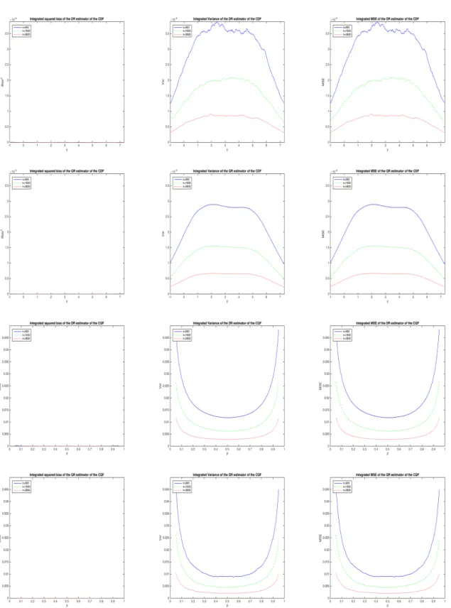
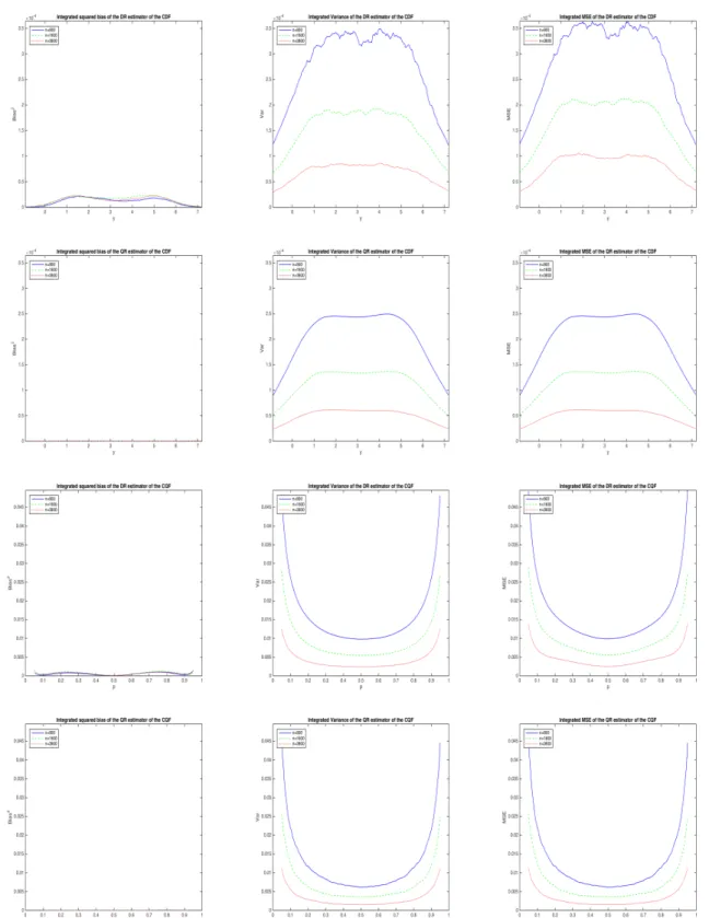
Figures 2–6 present, for each type of DGP, a few summaries of the Monte Carlo distribution of the monotonic estimators ˆF_n+ and ˆF_n◦ as functions of the cutoff level y, and of the monotonic estimators

7_{In principle,}

Jshould increase with the sample size, but for our Monte Carlo experiment we found that a fine enough fixed grid was a good choice. Our choice of a grid ofJ=199 points is the result of some experimentation. Reducing the grid size increases the bias, increasing it slows down the computations. To check the validity of our choice ofJ, we performed 1000 simulations from the logistic linear location model with finer grid sizes for the largest sample (J=397 andJ=793) and found no difference in the bias and variance of all estimators. Results are available upon request.

(17)

ˆ

Q+_n and ˆQ◦_n as functions of the quantile level p. The summaries considered are the squared bias, the variance and the MSE, all averaged over the distribution of X. Each panel in a figure compares the results obtained from samples of increasing size (n=900, 1600 and 3600) drawn from the same DGP. Tables 1–5 focus on our two monotonic estimators of the CQF, namely the DR estimator ˆQ+_n and the QR estimator ˆQ◦_n, and present their average squared bias and average variance at various quantile levels (p= .10, .25, .50, .75 and .90) for different sample sizes.8 The last two columns of each table present asymptotic calculations based on the results in Sections 2–4. To facilitate comparisons between the Monte Carlo results and the asymptotic calculations, we rescale all estimates multiplying bypn. Thus, care is needed when making comparisons across columns of a table corresponding to different sample sizes.

The results for the logistic linear location model are presented in Table 1, separately forβ = 2π andβ=6π, corresponding respectively to a medium (.50) and a high (.90) value of the regressionR2. To save space, the results for the other DGPs discussed in Section 4.2 are presented in Tables 2–5 for β=2πonly. In line with our asymptotic framework, we allow the degree of misspecification to change with the sample size by settingδ=c/pnfor different values ofc.9

Before discussing specific results for each DGP, we briefly summarize some findings that are common across DGPs. First, the profiles of the average variance are different for estimators of the CDF and the CQF: for the former they have an inverted U-shape with evidence of asymmetry and bimodality, for the latter they instead have a nice symmetric U-shape with a minimum near p=.50. Second, ˆF_n◦and ˆQ+_n have smoother average variance and MSE profiles than ˆF_n+ and ˆQ◦_n, especially when the sample size is relatively small (n=900), which reflects the fact that the former are obtained by integration, the latter by inversion. Third, the DR estimators ˆF_n+ and ˆQ+_n are always less precise (i.e., have higher average variance) than the QR estimators ˆF_n◦ and ˆQ◦_n. Thus, the DR estimators are more efficient (i.e., have lower average MSE) than the QR estimators only in a few cases when they are substantially less biased (i.e., have lower average squared bias) than the QR estimators. Fourth, the asymptotic approximations to bias and variance are quite accurate, i.e., close to the Monte Carlo biases and variances, even for relatively small samples, except perhaps when yis near the tails ofY orpis close to 0 or 1. In particular, the average squared bias of all estimators and the ratio of their average squared bias to their average variance are roughly proportional to c2 for any value of n. Finally, changes in the value of β affect

8_{The corresponding tables for our two monotonic estimators of the CDF, ˆ}_F+

n and ˆFn◦, are available upon request. Tables are also available for the squared bias and the variance of ˆQ+_nand ˆQ◦_nat specific value ofx. Qualitatively, the results are very similar to those for the average squared bias and the average variance.

9_{We choose the values of}_c_{in such a way that}_δ_{is constant along the main anti-diagonal of the 3}

×3 table corresponding to the nine different combinations ofcandnthat we consider.

(18)

heavily the variance of the DR estimators, but only have a very small effect on the variance of the QR estimators. The effects of changes in the value ofβon the bias of the different estimators, and of changes in the value ofδandc on their bias and variance, vary instead with the form of misspecification. 5.2.1 Logistic linear location model

Figure 2 refers to the benchmark case withβ=2π. Since a linear specification is correct for both the CLF and the CQF, it is not surprising that all our estimators shows little evidence of bias. As a result, their average variance and MSE have essentially the same profiles.

Table 1 shows the average squared bias and the average variance of the DR estimatorpnQˆ+_n and the QR estimatorpnQˆ◦_nat various quantile levels, separately forβ=2πandβ=6π. The squared bias of ˆQ+_n is almost always slightly larger than the bias of ˆQ◦_n, while its variance is always larger than the variance of ˆQ◦_n. Notice that the squared bias and the variance of ˆQ+_n both increase withβ, especially in smaller samples (n=900). On the contrary, those of ˆQ◦_n do not change withβ. This is a consequence of the shift equivariance property of linear QR estimators (see e.g. Koenker 2005, p. 39), as the QR estimates of the intercept and the slope of model (3) when(α,β) = (0, 6π) are linked to those when

(α,β) = (0, 2π)by the relationships ˆα(0, 6π) =αˆ(0, 2π) and ˆβ(0, 6π) = βˆ(0, 2π) +4π. Since ˆQ◦_n is always more precise and is almost always less biased than ˆQ+_n, it emerges clearly as the estimator of choice. Further, consistently with earlier findings in Koenker, Leorato and Peracchi (2013), the relative advantage of the QR estimator in terms of efficiency increases withβ.

5.2.2 Omitted variables

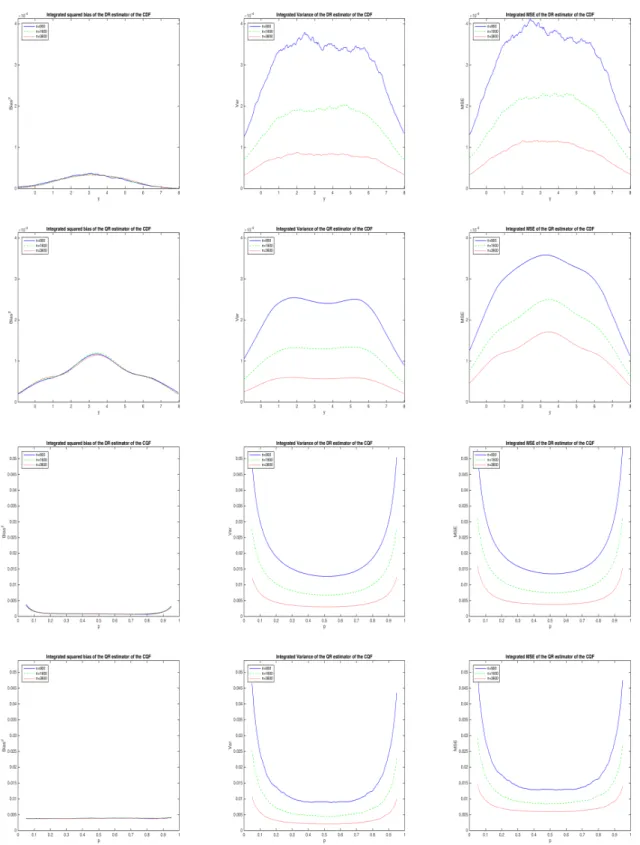
Figure 3 refers to the case when φ(x) = x2 andδ= 10. Since our estimators omit a quadratic term, they are all biased. The average squared bias of ˆF_n+ and ˆF_n◦has an invertedU-shape with a peak at the center of the distribution of Y, while that of ˆQ+_n and ˆQ◦_n changes little withp. The DR estimators ˆF_n+ and ˆQ+_n have less bias than the QR estimators ˆF_n◦and ˆQ◦_n, but they are also less precise, so their MSE is actually larger than that of the QR estimators when n=900 and is only slightly smaller for larger sample sizes.

Table 2 shows the values of the average squared bias and variance of pnQˆ+_n andpnQˆ◦_n when the degree of misspecification is δ= c/pn, for different values of c and n. Notice that, in line with the asymptotic calculations, the average squared bias of ˆQ◦_nchanges very little withp. Increasingcincreases by about c2 the average squared bias of both estimators, and therefore also the ratio between their average squared bias and their average variance. For example, whenp=.50 andn=1600, doubling

(19)

c from 30 to 60 increases the average squared bias from 3.51 to 14.05 for ˆQ◦_n and from .73 to 2.56 for ˆ

Q+_n. It also increases the ratio between the average squared bias and the average variance from .48 to 1.91 for ˆQ◦_nand from .07 to .23 for ˆQ+_n.

From the table we can also compute the average squared bias and variance of ˆQ+_nand ˆQ◦_nat any given quantile level pwhenδis kept constant but ngrows. The results are again in line with the asymptotic calculations. For example, whenβ =2π andδ= c/pn= 1, reading along the anti-diagonal shows that the average squared bias of ˆQ◦_natp=.50 changes only marginally from 3.494/900=.00388 when n = 900 to 13.866/3600= .00385 when n= 3600. On the contrary, the average variance of ˆQ◦_n at p = .50 falls from 8.179/900 = .0091 when n= 900 to 7.433/3600 = .0021 when n= 3600. The latter value represents 22.7 percent of the average variance whenn=900, very close to the value of 25 percent based on the asymptotic calculations.

The table shows that the relative advantage of ˆQ+_n in terms of lower bias falls withnbut increases withc. In line with the asymptotic calculations, it also falls as p moves towards 0 or 1. On the other hand, the relative disadvantage of ˆQ+_n in terms of lower precision changes little withnor c, but falls as pmoves towards 0 or 1.

5.2.3 Heteroskedasticity

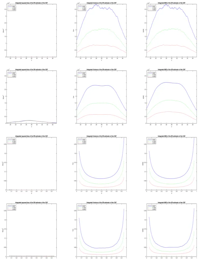
Figure 4 refers to the case whenσ_δ(x) =1+δx2, withδ=1/6, that is, the scale function is quadratic in x. Except for ˆQ◦_nwhenp=.50, all estimators are biased, as a linear specification of the CLF or the CQF is generally incorrect under this form of heteroskedasticity.10 However, the DR estimators ˆF_n+ and ˆQ+_n are both more biased and less precise than the QR estimators ˆF_n◦and ˆQ◦_n, so they are clearly dominated in terms of MSE.

Table 3 shows the values of the average squared bias and variance of pnQˆ+_n andpnQˆ◦_n when the degree of misspecification is δ = c/pn, for different values of c and n. As in the omitted variables case, increasingcincreases by aboutc2the average squared bias of both estimators, and therefore also the ratio between their average squared bias and their average variance. For example, whenp =.10 andn=900, doubling cfrom 5 to 10 increases the average squared bias from .48 to 1.91 for ˆQ◦_n and from 2.66 to 11.21 for ˆQ+_n. It also increases the ratio between the average squared bias and the average variance from .02 to .08 for ˆQ◦_n and from .10 to .38 for ˆQ+_n.

The relative disadvantage of ˆQ+_n in terms of bias changes little withnbut, in line with the asymptotic calculations, changes a lot withpandc, and is especially large whenp=1/2 (the quantile level at which 10_{Results for other forms of heteroskedasticity where one of the two approaches (either DR or QR) remains consistent are}

(20)

the QR estimator ˆQ◦_n is consistent by the symmetry of the logistic distribution). On the other hand, the relative disadvantage of ˆQ+_n in terms of precision changes little withn,pandc.

5.2.4 Nonlogistic models

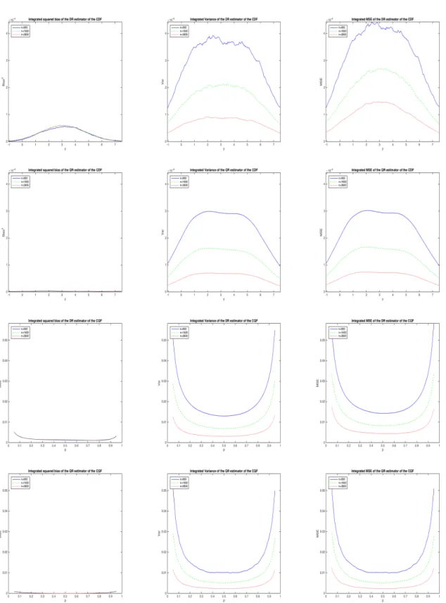
Figure 5 refers to the case when the DGP is of the form (3) but the error is a mixture(1₋δ)_∗U+δ_∗T, whereδ=1/4,U is distributed as standard logistic, and T is distributed as Student t with 3 degrees of freedom. The DR estimators ˆF_n+ and ˆQ+_n are biased, as a linear specification is correct for the CQF but not for the CLF, and their average squared bias has a bimodal profile. This bimodality is in line with the asymptotic calculations as in this caseΨ(x,u) =ζ(u), whereζ(u) = (Λ(u)−G(u))/λ(u)andG(u) denotes the distribution function of a Student t, and the square ofζ(u)is bimodal. Notice that there is also some evidence of bias for ˆF_n◦. Overall, the DR estimators are both more biased and less precise than the QR estimators, so they are clearly dominated in terms of MSE.

Table 4 shows the values of the average squared bias and variance of pnQˆ+_n andpnQˆ◦_n when the mixing probability is δ = c/pn, for different values of c and n. Since the bias of ˆQ◦_n falls with n, the relative disadvantage of ˆQ+_n in terms of bias increases with n. It also varies a lot with p andc, in accordance with the asymptotic calculations.

We obtain qualitatively similar results when the error in model (3) is distributed asymmetrically as a mixture of the standard logistic and the standard Gumbel, the main difference being that now the bias and the variance of the DR estimators are no longer symmetric.11

5.2.5 Transformation models

Figure 6 refers to the case when the DGP is a Box-Cox transformation model of the form Y(1−δ)+1= α+βX+U, withδ=1/4 andβ=2π. We also setα=4πto guarantee thatZ=α+βX+U is almost always nonnegative so, for anyδ ₆= 1, the inverse transformation Y = [δ+ (1₋δ)Z]1/(1−δ) returns almost always a real number. Now the QR estimators ˆF_n◦ and ˆQ◦_n are biased, as a linear specification is correct for the CLF but not for the CQF, and the average squared bias of ˆF_n◦has an inverted U-shape with a peak at the center of the distribution ofY, while that of ˆQ◦_nis relatively small and changes little withp. Although the DR estimators ˆF_n+ and ˆQ+_n have almost no bias, they are always much less precise than the QR estimators, so their MSE is actually larger than the MSE of the QR estimators.

Table 5 shows the values of the average squared bias and variance of pnQˆ+_n andpnQˆ◦_n when the degree of misspecification isδ=c/pn, for different values ofcandn. The results support the graphical

(21)

evidence from Figure 6. In particular, even in the worst case for ˆQ◦_n(namelyc=2,p=.10 andn=900), the ratio of its MSE to the MSE of ˆQ+_n is equal to .851.

6

Conclusions

In this paper we presented asymptotic results and Monte Carlo evidence on the sampling properties of monotonic CDF and CQF estimators obtained from the DR approach under the assumption that the CLF is linear in parameters and from the QR approach under the assumption that the CQF is linear in parameters. We considered both cases when the underlying linear-in-parameter models are correctly specified and several types of model misspecification of considerable practical relevance.

Our results may be summarized as follows. First, the profiles of the average variance are different for estimators of the CDF and the CQF: for the former they have an inverted U-shape, with evidence of asymmetry and bimodality, for the latter they instead have a nice symmetric U-shape even for relatively small samples (n=900).

Second, estimators obtained by rearrangement ( ˆF_n◦ and ˆQ+_n) have smoother average variance and MSE profiles than estimators obtained by inversion ( ˆF_n+and ˆQ◦_n), especially in smaller samples.

Third, the main advantage of the DR approach relative to the QR approach is that it produces es-timators that are less biased (i.e., have lower average squared bias) in some settings. These include the cases when the assumed model ignores a quadratic term in the conditional mean or the need of monotonically transforming the outcome of interest. On the other hand, QR estimators are less biased when the assumed model ignores the presence of heteroskedastic or nonlogistic errors.

Fourth, DR estimators are always less precise (i.e., have higher average variance) than QR estima-tors. Thus, the only case when they are more efficient (i.e., have lower average MSE) than QR estimators is when they have substantially less bias. In our Monte Carlo experiments this only occurs when the assumed models omit a quadratic term in the conditional mean.

Fifth, the asymptotic approximations to bias and variance are quite accurate, even for relatively small samples, except perhaps when y is near the tails of Y or pis close to 0 or 1.

We hope that our results provide guidance to practitioners about the choice between the DR and the QR approach. Of course, when it comes to choosing between the two approaches, other aspects may also matter besides the sampling properties in finite or in large samples. One important aspect is the possibility of generalizing to the case whenY is discrete, or subject to censoring, or multivariate. Another is the presence of censoring or mass points in the distribution of the outcome of interest. In both these cases, which we leave for future research, the DR approach may look more natural.

(22)

References

Angrist J., Chernozhukov V., and Fernández-Val I. (2006). Quantile regression under misspecification, with an application to the U.S. wage structure. Econometrica, 74: 539–563.

Azzalini A. (1981). A note on the estimation of a distribution function and quantiles by a kernel method. Biometrika, 68: 326–328.

Chernozhukov V., Fernández-Val I., and Galichon A. (2007). Quantile and probability curves without crossing. CeMMAP Working Paper CWP 10/07.

Chernozhukov V., Fernández-Val I., and Galichon A. (2010). Quantile and probability curves without crossing. Econometrica, 78: 1093–1125.

Chernozhukov V., Fernández-Val I., and Melly B. (2013). Inference on counterfactual distributions. Econometrica, 81: 2205–2268.

Dette H., and Volgushev S. (2008). Non-crossing nonparametric estimates of quantile curves. Journal of the Royal Statistical Society, Series B, 70: 609–627.

Foresi S., and Peracchi F. (1995). The conditional distribution of excess returns: An empirical analysis. Journal of the American Statistical Association, 90: 451–466.

Fortin N., Lemieux T., and Firpo S. (2011). Decomposition methods in economics. In O. Ashenfelter and D. Card (eds.),Handbook of Labor Economics, Vol. 4 A, 1–102.

Hall P., and Müller P.-G. (2003). Order-preserving nonparametric regression, with application to condi-tional distribution and quantile function estimation.Journal of the American Statistical Association, 98: 598–608.

Hall P., Wolff R.C.L., and Yao Q. (1999). Methods for estimating a conditional distribution function. Journal of the American Statistical Association, 94: 154–163.

Hothorn T., Kneib T., and Bühlmann P. (2014). Conditional transformation models. Journal of the Royal Statistical Society–Series B, 76: 3–37.

Koenker R., and Bassett G. (1978). Regression quantiles. Econometrica, 46: 33–50. Koenker R. (2005). Quantile Regression. Cambridge University Press: New York.

(23)

Koenker R., Leorato S., and Peracchi F. (2013). Distributional vs. quantile regression. EIEF Working Paper 13/29.

Koenker R., and Xiao Z. (2002). Inference on the quantile regression process,Econometrica, 70: 1583– 1612.

Leorato S., and Peracchi F. (2015). Shape regressio