Kent Academic Repository
Full text document (pdf)
Copyright & reuse
Content in the Kent Academic Repository is made available for research purposes. Unless otherwise stated all content is protected by copyright and in the absence of an open licence (eg Creative Commons), permissions for further reuse of content should be sought from the publisher, author or other copyright holder.
Versions of research
The version in the Kent Academic Repository may differ from the final published version.
Users are advised to check http://kar.kent.ac.uk for the status of the paper. Users should always cite the published version of record.
Enquiries
For any further enquiries regarding the licence status of this document, please contact: [email protected]
If you believe this document infringes copyright then please contact the KAR admin team with the take-down information provided at http://kar.kent.ac.uk/contact.html
Citation for published version
Brookhouse, James and Otero, Fernando E.B. (2018) Post-Processing Methods to Enforce Monotonic
Constraints in Ant Colony Classification Algorithms. In: 2018 International Joint Conference
on Neural Networks, 8-13 July 2018, Rio de Janeiro, Brazil. (In press)
DOI
Link to record in KAR
http://kar.kent.ac.uk/67177/
Document Version
Post-Processing Methods to Enforce Monotonic
Constraints in Ant Colony Classification Algorithms
James Brookhouse
School of Computing University of Kent Chatham Maritime, UK Email: [email protected]Fernando E. B. Otero
School of Computing University of Kent Chatham Maritime, UK Email: [email protected]Abstract—Most classification algorithms ignore existing do-main knowledge during model construction, which can decrease the model’s comprehensibility and increase the likelihood of model rejection due to users losing trust in the models they use. One approach to encapsulate this domain knowledge is monotonic constraints. This paper proposes new monotonic pruners to enforce monotonic constraints on models created by an existing ACO algorithm in a post-processing stage. We compare the effectiveness of the new pruners against an existing post-processing approach that also enforce constraints. Additionally, we also compare the effectiveness of both these post-processing procedures in isolation and in conjunction with favouring con-straints in the learning phase. Our results show that our pro-posed pruners outperform the existing post-processing approach and the combination of favouring and enforcing constraints at different stages of the model construction process is the most effective solution.
I. INTRODUCTION
Data mining focuses on the automated search for useful patterns in data [1]. Classification is the most studied task in data mining, where the problem involves a set of instances— each instance is described by a set of predictor attribute values with an associated target class value. The goal of a classification algorithm is to find the best classifier that accurately represents the relationships between predictor and class attribute values, and therefore classification problems can be viewed as optimisation problems. There are many classifi-cation algorithms in the literature, in many of these algorithms they concentrate on producing accurate models at the expense of other goals. Accuracy is an important goal, however, there are other goals that exist. These other goals can be just as important or more important depending on the application. Alternative goals can include a model’s comprehensibility, or its ability to preserve existing domain knowledge. These features can contribute towards model acceptance by domain experts.
Model rejection by domain experts is a possibility if a model does not preserve existing patterns as it would seem counter intuitive. Hoover and Perez [2] state that the economic field scepticism towards data mining as a technique to search for models is due to the discovery of accidental correlations: “Data mining is considered reprehensible largely because the world is full of accidental correlations, so that what a search turns up is thought to be more a reflection of what we want to
find than what is true about the world.”[2, p. 197]. Semantic constraints allow model construction to be guided by providing information on real correlations present within the data. While there are a number of different semantic constraint types, we explore the implementation of monotonic constraints in the discovery of classification rules.
In this paper we have focused on one particular encapsula-tion of domain knowledge, monotonic constraints. Monotonic constraints are simple relationships that guide the creation of models. We compared an existing post-processing additive monotonic approach, which enforces monotonic constraints by adding conditions to the model, against a new set of post-processing pruners that remove conditions from a model to enforce constraints. We also investigate the reliance on purely post-processing steps to enforce these constraints, or if constraints should be incorporated into the learning phase as soft constraints. This is achieved with the use of an ACO-based rule learner, which is able to favour monotonic constraints during the model construction.
The rest of this paper is structured as follows. Firstly, Section II summarises the existing work from the literature. Section III describes the existing ACO algorithm that favours monotonic constraints in the learning phase along with the suite of monotonic pruners that can be applied in the post-processing phase. Section IV presents our results on thir-teen UCI Machine Learning datasets, including a comparison between four monotonic ACO-based algorithms. Finally, we discuss our results and present our conclusions and possible future research directions in Section V.
II. BACKGROUND
A. Ant Colony Classification Algorithms
The first ACO classification algorithm, called Ant-Miner, was proposed in [3]. Ant-Miner follows a sequential covering strategy, where individual rules are created by an ACO pro-cedure, then data instances that are covered by the rule are removed from the training data. The main idea is to search for the best classification rule given the current training data at each iteration of the sequential covering. Ants traverse a construction graph selecting terms to create a rule in the form
IF term1 AND ... AND termn THEN class, where
TABLE I
SIMPLE HOUSE RENTAL DATA SET. THE DEPENDENT ATTRIBUTE IS THE
RENTALVALUE WHILEFLOORAREA ANDLOCATION ARE INDEPENDENT ATTRIBUTES
Target Attribute Predictor Attributes Rental Value Floor Area Location
Medium 45 2
High 80 1
Low 33 3
Medium 65 2
High 100 2
the class prediction. Each ant starts with an empty rule and iteratively selects terms to add to its partial rule based on their values of the amount of pheromone τ and a problem-dependent heuristic information η, similarly to Ant System (AS) [4]. Following on Ant-Miner’s success, many extensions have been proposed in the literature [5]: they involve different rule pruning and pheromone update procedures, new rule quality measures and heuristic information.
One potential drawback of using sequential covering to cre-ate a list of rules is that there is no guarantee that the best list of rules is created. Ant-Miner (and the majority of its extensions) perform a greedy search for the list of best rules, using an ACO procedure to search for the best rule given a set of data instances, and it is highly dependant on the order that rules are created. Therefore, they are limited to creating thelist of best rules, which does not necessarily corresponds to the best list of rules.cAnt-MinerPBis an ACO classification algorithm that employs an improved sequential covering strategy to search for the best list of classification rules [6]. While Ant-Miner uses an ACO procedure to create individual rules in a one-at-a-time (sequential covering) fashion, cAnt-MinerPB employs an ACO procedure to create a complete list of rules. Therefore, it can search and optimise the quality of a complete list of rules instead of individual rules—i.e., it is not concerned by the quality of the individual rules as long as the quality of the entire list of rules is improving.
B. Monotonic Constraints
When existing domain knowledge is available, monotonic constraints can incorporate this knowledge into the construc-tion of new models. For example, if you consider house rent the price can/will depend on the location and floor area. Table I shows a simple hypothetical rental dataset. One relationship in this data set is that houses in better locations (lower values of attribute Location) increase their rental price. This is the case for all possible pairs in the data set.
Monotonicity is found in many different fields including house/rental prices, medicine, finance and law. Looking at the first example of rental prices, it can be expected that as the location of a property becomes better (lower value of Location) its rental value will also increase—this can be seen in the example data shown in Table I. The majority of classification algorithms are not monotonically aware and do not enforce this relationship during model construction, yet
still produce good models. However, if models violate these constraints they may not be accepted by experts as valid, and therefore, conforming to monotonicity constraints may help improve model acceptance [7], [8].
Monotonicity can be defined formally in the following manner. LetX =X1× X2× · · · × Xi be the instance space of iattributes,Y be the target space, and functionf :X → Y. It is also assumed that both the instance space and target space have an ordering. A function can then be considered monotone if:
∀x,x′∈ X :x≤x′ =⇒ f(x)≤f(x′) , (1) where x and x′ are two vectors in instance space, x =
(x1, x2,· · ·, xi)[9]. In other words,f(x)is monotonic if and only if all the pairs of examples x, x′ are monotonic with respect to each other.
C. Enforcing Monotonicity Constrains
Monotonicity can be enforced in a number of different stages in the data mining process. In the model construc-tion stage the algorithm creates monotonic models, possibly constraining the search. Also, constraints can be enforced in a post-processing stage via the modification of constructed models to enforce monotonic constraints.
Constraints also appear in two different forms hard or soft. Hard constraints are enforced rigidly and will reject any new model or change to an existing model that would cause a violation. Good models can be rejected due to small violations in their monotonicity when this hard constraint method is used. The second method, soft constraints, balances the monotonicity of a model against its quality, allowing small violations to exist if they sufficiently increase the quality—i.e., monotonic constraints are favoured.
1) Model Construction: Soft constraints have been imple-mented in the model construction stage by Ben-David [10]. Ben-David assigns a non-monotonicity index to each tree produced. This index is the ratio between the number of non-monotonic leaf node pairs and the maximum number of pairs that could have been non-monotonic.
First, a non-monotonic n-dimensional matrix constructed where n is the number of branches in the tree. This matrix is used to find the number of violations in the current tree, and used to find the tree’s non-monotonicity index. The non-monotonicity index can be converted to an ambiguity score and then incorporated with the tree’s accuracy score. The accuracy of the models produced were not significantly degraded compared to the original algorithm, however the combined metric did produce fewer models that breached the monotonicity constraints [10].
Ben-David has also investigated monotonic ordinal clas-sifiers, proposing the hypothesis that adding monotonicity constraints to learning algorithms will impair their accuracy against those that do not. Ordinal classifiers are classifiers that allow discrete categories to have an order, for example credit rating has an obvious order if the categories are poor, ac-ceptable and good. There were two unexpected results. It was
found that ordinal classifiers did not significantly improve their accuracy over non-ordinal classifiers. Secondly, the monotonic algorithms were not able to significantly outperform a simple majority-based classifier. It is theorised that these results were due to noisy data sets: the monotonic classifiers enforced hard constraints, in the presence of noisy data a softer approach may lead to better results [11].
Brookhouse and Otero have introduced two ACO-based algorithms cAnt-MinerPB+MC [12] and Ant-Miner-RegMC [13] that enforce monotonicity constraints for the classification and regression task, respectively. Both algorithms enforced soft constraints during rule construction by incorporating a measure of monotonicity into a rule’s quality, which is then incorporated into the pheromone matrix of the ant colony. In cAnt-MinerPB+MC, a naive pruner is used to enforce hard constraints in a post processing step—cAnt-MinerPB+MC is discussed in more detail in Section III-A.
2) Post-Processing: Feelders [8] has suggested that using non-monotonic criteria in tree construction is not beneficial as splits later in the construction process can transform a tree from a state of non-monotonicity to one that is. Therefore, Feelders has suggested several pruning methods to make the minimal number of changes to make a tree monotonic in a post-processing phase [8].
The first proposed pruner is the Most Non-monotone Parent (MNP) method, which aims to prune the node that gives the most number of monotone pairs. This method has the disadvantage of possibly creating more non-monotonic pairs than it removes leading to a net increase in non-monotonicity. The second method proposed is the Best Fix (BF) method, which prunes the node that gives the biggest reduction in non-monotonicity. While it solves the problem with the first pruner, it is more computationally expensive. The authors have also combined these pruning methods with existing complexity pruning methods and found that the monotonic trees produced no significant difference in performance compared to trees produced without monotonic pruning. However, it was ob-served that the trees produced were smaller, which aids the comprehensibility of the models produced further [8].
3) Additive monotonic post-processing with RULEM: Ver-beke et al. introduced a new algorithm, RULEM [14], that tackles the monotonic problem in a different way. While still a post-processing technique, RULEM adds additional new rules to the list of rules to force monotonic behaviour. One advantage of RULEM is any learning algorithm that can produce a model that can be transformed into a list of rules can be fixed and made monotonic.
RULEM fixes a list of rules by adding new rules to fix any non-monotonic features. RULEM first creates an n -dimensional matrix, wherenis the number of attributes in the solution space. Rules from the original list of rules are then added to this solution space, claiming the regions that they cover. Any non-monotonic region can then be identified and rules iteratively generated to fix these regions with respect to the existing rules. Finally these rules are compacted to reduce the number of rules added. The new compacted rules
are then added to the top of the rule list to ensure they create a monotonic list of rules.
III. DISCOVERINGMONOTONICCLASSIFICATIONRULES
This section provides an overview of cAnt-MinerPB and the soft constraints found in cAnt-MinerPB+MC. Finally, an overview of the proposed hard pruning strategy found inc Ant-MinerPB+MCP. A high-level pseudocode of these algorithms is shown in Algorithm 1, where the differences among them are highlighted.
A. cAnt-MinerPB with monotonicity constraints
As we discussed in Section II-A,cAnt-MinerPB is an ACO classification algorithm that employs an improved sequential covering strategy to search for the best list of classification rules. In summary,cAnt-MinerPB works as follows. Each ant starts with an empty list of rules and iteratively adds a new rule to this list. In order to create a rule, an ant adds one term at a time to the rule antecedent by choosing terms to be added to the current partial rule based on the amount of pheromone (τ) and a problem-dependent heuristic information (η). Once a rule is created, it undergoes a pruning procedure. Pruning aims at removing irrelevant terms that might be added to a rule due to the stochastic nature of the construction process: it starts by removing the last term that was added to the rule and the removal process is repeated until the rule quality decreases when the last term is removed or the rule has only one term left. Finally, the rule it is added to current list of rules and the training examples covered by the rule are removed.1 An ant
creates rules until the number of uncovered examples is below a pre-defined threshold.
At the end of an iteration, when all ants have created a list of rules, the best list of rules (determined by an error-based list quality function) is used to update pheromone values, providing a positive feedback on the terms present in the rules—the higher the pheromone value of a term, the more likely it will be chosen to create a rule. This iterative process is repeated until a maximum number of iterations is reached or until the search stagnates.
cAnt-MinerPB+MC is an extension ofcAnt-MinerPB which incorporates monotonic constraints into the model construc-tion phase and post processing. It takes advantage of c Ant-MinerPB’s global list construction when optimising for both accuracy and monotonicity. This is achieved by modifying the quality function to include a monotonic correctness function along with the conventional accuracy based measure (line 16)—this is the same function that is used in the soft pruner and shown by equations 2 and 3. Line 12 shows the addition of a soft pruner that uses a modified quality function to prune the rules during the construction phase, which will be discussed in detail in Section III-B. This soft rule pruner replaces the rule pruner present in cAnt-MinerPB. cAnt-MinerPB+MCP also adds a hard monotonic pruner (line 26) to enforce monotonic
1An example is covered by a rule when it satisfies all terms (attribute-value
Algorithm 1: High-level pseudocode of the c Ant-MinerPB+MC(P) algorithm. The main differences com-pared tocAnt-MinerPB [6] are found on lines 12, 16 and 26.
Input: training instances
Output: best discovered list of rules 1. InitialisePheromones();
2. listgb← {};
3. t←0;
4. whilet < maximum iterationsand not stagnationdo 5. listib← {};
6. forn←1 to colony sizedo
7. instances←all training instances; 8. listn← {};
9. while|instances|>maximum uncovereddo 10. ComputeHeuristicInformation(instances); 11. rule ←CreateRule(instances);
12. SoftPruner(rule, listn);
13. instances←
instances−Covered(rule, instances); 14. listn←listn+rule;
15. end while
16. ifQuality(listn)> Quality(listib)then
17. listib←listn;
18. end if
19. end for
20. U pdateP heromones(listib);
21. ifQuality(listib)> Quality(listgb)then
22. listgb←listib; 23. end if 24. t←t+ 1; 25. end while 26. HardPruner(listgb); 27. return listgb;
constraints rigidly ensuring the final model will always be monotonic.
In ACO terms, a pruner is a local search operator. Dur-ing rule construction a soft pruner is used to influence the pheromone matrix and therefore the decisions of the colony towards good monotonic solutions. By softly enforcing monotonic constraints globally within the ACO stage, the optimisation of monotonicity should reduce the need to rely on the more aggressive and potentially more damaging hard pruners later on.
B. Soft Rule Pruning
A soft monotonic prune allows violations in the monotonic constraint if the consequent improvement in accuracy is large enough. The pruner operates on an individual rule and iter-atively removes the last term until no improvement in the rule quality is observed. Applying a soft pruner during model creation allows the search to be guided towards monotonic models while still allowing exploration of the search space.
As monotonicity is a global property of the model, the rule being pruned is temporarily added to the current partial list of rules, its non-monotonicity index (NMI) can then be used as a metric to assess the rules monotonicity and it is given by:
N M I = Pk i=1 Pk j=1mij k2−k , (2) where mij is 1 if the pair of rules rulei and rulej violate
the constraint and 0 otherwise; k is the number of rules in the model. The NMI of a model is constrained between zero and one: it calculates the ratio of monotonic violating pairs over the total possible number of prediction pairs present in the model being tested, the lower a NMI is the better a model is considered. If this is the first rule in the partial model it will be automatically designated monotonic and be assigned a non-monotonicity index of zero. The NMI is then incorporated into the quality metric by:
Q= (1−ω)·Accuracy+ω·(1−N M I) , (3)
where Q is the quality of a model and ω is an adjustable weighting that sets the importance of monotonicity and ac-curacy to the overall rule quality. Note that Equation 3 can be used to calculate the quality of either a single rule (used during the soft pruner, line 12 of Algorithm 1) or a complete list of rules (line 16 and 26 of Algorithm 1).
C. Hard List Pruning
Monotonicity is a global property of a model as it requires at least two rules to create a violation. Therefore, pruners that operate on a global rule list are preferential to those operating on an individual rule which can only modify a single rule to fix the violations present in the model [15]. The original cAnt-MinerPB+MC algorithm contained a single monotonic backtrack pruner, now referred to as the Naive Pruner (NP). The Naive Pruner can be very destructive if the violating rule occurs towards the top of a rule list as the bottom section of the list is discarded. To counteract these affect we propose two new pruners: the Most Violations Pruner (MVP) and the Best Fix Pruner (BFP). The three list pruners now work in conjunction to increase the accuracy of the model returned bycAnt-MinerPB+MC: all three pruners are applied in turn to the constructed list and the pruner that achieves the highest accuracy on the training set is used for the final prune.
1) Naive Pruner: The hard monotonic pruner enforces the monotonic constraints rigidly. It operates on a list of rules as follows: (1) the NMI of a list is first calculated (Equation 2); (2) if it is non zero, the last term of the final rule is removed or, if the rule contains no terms, the rule is removed; (3) the NMI is then recalculated for the modified list of rules. This is repeated until the NMI of the rule list is zero. Finally the default rule is added to the end of the list if it has been removed and the new monotonic rule list is returned. The pseudocode for the naive pruner is shown in Algorithm 2.
Algorithm 2: Pseudocode for the Naive Pruner, where a term is removed from the list until the NMI is zero.
Input: list
Output: list
1: whileNMI(list)>0 do 2: PruneLastTerm(list);
3: ifLastRuleLength(list) == 0then 4: RemoveLastRule(list);
5: end if 6: end while 7: return list;
Algorithm 3:Pseudocode for the Most Violations Pruner, in each iteration the rule with the worst NMI has its last term removed.
Input: list
Output: list
1: whileNMI(list)>0 do 2: ruleworst← {};
3: forn← 1to listsize do
4: ifNMI(rulen)≥NMI(ruleworst)then
5: ruleworst←rulen;
6: end if
7: end for
8: PruneFinalTerm(ruleworst);
9: ifRuleLength(ruleworst) == 0then
10: RemoveRule(list, ruleworst);
11: end if 12: end while 13: return list;
2) Most Violations Pruner (MVP): This pruner prunes the worst rule in terms of NMI in the list of rules. It calculates the NMI of each rule using Equation 2 and the rule with the highest NMI has its final term removed. The NMI of each rule is then recalculated and the procedure continues until the model’s NMI is 0. In the case of a draw—e.g., with a single pair of rules violating each other—the rule appearing lower in the list is preferentially pruned. This decision is made as rules towards the top of the list were generated on the full training set and therefore likely to be more powerful than those towards the end which are classifying fewer remaining instances. The pseudocode for the MVP pruner is shown in Algorithm 3.
3) Best Fix Pruner (BFP): The third global pruner attempts to fix the rule that would give the greatest reduction in the model’s NMI. The pseudocode for the best fix pruner is shown in Algorithm 4. Each non-monotonic rule in the complete model is pruned backwards from the last term until a change in the model’s NMI is detected. The pruned rule that led to the largest decrease in NMI is kept, the remaining rules are restored to their original state. This process is repeated until the model becomes monotonic. For the same reasons explained in the MVP approach, draws are solved by pruning the rule lower in the list.
Algorithm 4:Pseudocode for the Best Fix Pruner, in each iteration the rule that will decrease the NMI by the largest amount will be pruned.
Input: list
Output: list
1: while NMI(list)>0 do 2: rulebi← {};
3: best improvement←0; 4: forn ←1 tolist sizedo
5: ruleprune←PruneRule(rulen);
6: improvement←NMI(list)−NMI(listprune);
7: if improvement≥best improvementthen 8: rulebi←rulen;
9: best improvement←improvement;
10: end if
11: end for
12: rulebi←PruneRule(rulebi);
13: end while 14: return list;
D. Monotonic Pruning Walkthrough
While the global optimisation of monotonicity when the ant colony generates a list of rules should reduce the need for additional aggressive pruning, the two new pruners aim to reduce the potential destructive affects further. Consider the following example, using a car efficiency dataset with a constraint that more powerful cars will have a lower efficiency. An execution of cAnt-MinerPB+MC would possibly produce the list of rules below:
1) IF Power ≥ 250 THEN High
2) IF Cylinders = 6 AND Power ≤ 200 THEN Low 3) IF Doors = 2 THEN Medium
4) IF Power ≤ 200 THEN High 5) IF <empty> THEN Medium
We can see that there is a monotonic violation between rules 1 and 2 as a car with a lower power can have a worse fuel efficiency (rule 2) than one with more power (rule 1). To ensure monotonicity, the Naive pruner would produce the following monotonic rule list (with the default rule being automatically re-added to ensure full coverage):
1) IF Power ≥ 250 THEN High 2) IF Cylinders = 6 THEN Low 3) IF <empty> THEN Medium
while the more sophisticated monotonic pruners MVP and BFP would produce the following monotonic rule list: 1) IF Power ≥ 250 THEN High
2) IF Cylinders = 6 THEN Low 3) IF Doors = 2 THEN Medium 4) IF Power ≤ 200 THEN High 5) IF <empty> THEN Medium
As can be seen, this is a far less destructive change than the Naive pruner, which would potentially induce a smaller change in the rule lists predictive accuracy.
TABLE II
DATA SETS FROM THEUCI [16]USED IN EXPERIMENTS,INCLUDING ATTRIBUTE AND CONSTRAINTS INFORMATION. THE CONSTRAINTS INFORMATION CONTAIN THE ATTRIBUTE NAME,DIRECTION OF CONSTRAINT,EITHER↑(INCREASING)OR↓(DECREASING),AND ITS CORRESPONDINGNMI.
Attributes Constraint
Name Size Nominal Continuous Attribute Direction NMI
Abalone 4176 1 7 Shell Weight ↑ 0.8062
Australian Credit 689 9 6 A8 ↓ 0.9925
Bank Marketing 4520 9 7 Loan ↓ 0.9859
Cancer 698 0 10 USize ↑ 0.0059
Car 1727 6 0 Safety ↑ 0.0460
Credit Screen 689 9 6 A4 ↑ 0.9444
German Credit 689 9 6 Credit History ↓ 0.9189
Haberman 305 0 3 PosNode ↑ 0.0861
MPG 397 0 7 Horsepower ↓ 0.0566
Pima 767 0 8 PGC ↑ 0.0947
User Knowledge 402 0 5 PEG ↑ 0.9764
Wine 177 0 13 Flavanoids ↓ 0.964
Wine Quality 1598 0 11 Alcohol ↑ 0.8373
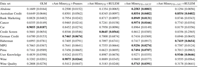
TABLE III
ACCURACY OF THE FIVE MONOTONIC RULE LEARNERS. OLMIS AN EXISTING MONOTONIC LEARNER,THE OTHER FOUR ALGORITHMS AREACO-BASED ALGORITHMS USING A COMBINATION OF SOFT CONSTRAINTS AND HARD CONSTRAINTS AT DIFFERENT STAGES OF THE CONSTRUCTION PROCESS. THE
BEST RESULT FOR EACH DATA SET IS SHOWN IN BOLD.
Data set OLM cAnt-MinerPB+Pruners cAnt-MinerPB+RULEM cAnt-MinerPB+MCP cAnt-MinerPB+MC+RULEM
Abalone 0.1609 [0.0164] 0.2500 [0.0152] 0.1354 [0.0065] 0.2583 [0.0083] 0.1294 [0.0056] Australian Credit 0.6449 [0.0646] 0.8501 [0.0562] 0.8345 [0.0097] 0.8554 [0.0402] 0.8554 [0.0402] Bank Marketing 0.8828 [0.0482] 0.7954 [0.0242] 0.8717 [0.0097] 0.8949 [0.0131] 0.8746 [0.0343] Cancer 0.8355 [0.0149] 0.9465 [0.0214] 0.7241 [0.0158] 0.9574 [0.0166] 0.7743 [0.0354] Car 0.9055 [0.0187] 0.8452 [0.0274] 0.7958 [0.0096] 0.8964 [0.0149] 0.8179 [0.0356] Credit Screen 0.5681 [0.0654] 0.8546 [0.0546] 0.8645 [0.0564] 0.8612 [0.0385] 0.8356 [0.2565] German Credit 0.6700 [0.0153] 0.7465 [0.0674] 0.7000 [0.6874] 0.7416 [0.0369] 0.6946 [0.0645] Haberman 0.6993 [0.0781] 0.7405 [0.0791] 0.7097 [0.6741] 0.7417 [0.0917] 0.7419 [0.0654] MPG 0.7663 [0.0367] 0.7641 [0.0641] 0.7555 [0.0664] 0.9256 [0.0274] 0.7587 [0.0124] Pima 0.7161 [0.0589] 0.7456 [0.0665] 0.6623 [0.0695] 0.7494 [0.0707] 0.7013 [0.0963] User Knowledge 0.4839 [0.0398] 0.9242 [0.0157] 0.8987 [0.0678] 0.9271 [0.0355] 0.9346 [0.0646] Wine 0.3202 [0.0201] 0.9875 [0.0264] 0.8889 [0.0345] 0.9605 [0.0377] 0.5555 [0.0564] Wine Quality 0.2808 [0.0276] 0.5412 [0.0447] 0.3183 [0.0248] 0.5743 [0.0391] 0.3178 [0.0641]
The three pruners are computationally inexpensive in com-parison to the main ACO optimisation stage, therefore a viable approach to rule list pruning is to combine all three pruners into a pruning suite where all pruners are evaluated on the training data and the rule list with the highest predictive accuracy on the training set is selected. At this point we can focus only on accuracy since all rule lists at this stage are guaranteed to be monotonic. This modified algorithm is called cAnt-MinerPB+MCP, using the soft constraints found incAnt-MinerPB+MCand the proposed pruning suite for hard constraints.
IV. RESULTS
Our results have been split into two sections, first we will present the monotonic algorithms and then compare the
best monotonic algorithm to traditional non-monotonic rule learners. As we are concentrating on rule induction and the comprehensible models that they produce, we will only be considering the performance of our algorithms against other rule induction methods. This allows a fair comparison remov-ing any biases that may be present due to model representation. In all experiments, cAnt-Miner variations were configured with a colony size of 5 ants, 500 iterations, minimum cases covered by an individual rule of 10, uncovered instance ratio of 0.01, and constraint weighting (ω) of 0.5 (only used by cAnt-MinerPB+MC). The eight chosen algorithms were tested on thirteen data sets taken from the UCI Machine Learning Repository [16]. Table II present the details of the chosen data sets, including a summary of the constraints used. All independent attributes had their NMI calculated to discover
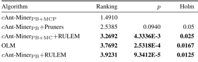
TABLE IV
AVERAGE RANKINGS ANDpVALUES OF THE MONOTONIC ALGORITHMS TESTED. RESULTS THAT SHOWED A STATISTICALLY SIGNIFICANT DIFFERENCE ACCORDING TO THEHOLMTEST FORα= 0.05ARE SHOWN
IN BOLD.
Algorithm Ranking p Holm
cAnt-MinerPB+MCP 1.4910
cAnt-MinerPB+Pruners 2.5385 0.0940 0.05
cAnt-MinerPB+MC+RULEM 3.2692 4.3336E-3 0.025
OLM 3.7692 2.5318E-4 0.0167
cAnt-MinerPB+RULEM 3.9231 9.3412E-5 0.0125
good monotonic relationships—the NMI results guided the choice of constrained attribute reported in the table.
A. Monotonic Experimental Results
To test the effectiveness of both additive and subtractive monotonic post-processing methods, four algorithms have been created: the first two usecAnt-MinerPBas the base with both the monotonic pruners and RULEM as post-processing steps; the other two algorithms usecAnt-MinerPB+MCas the base, which incorporates the soft constraints into the model construction and then uses either the monotonic pruners or RULEM to enforce the constraints rigidly.
These four algorithms have also been compared against OLM [11], a monotonic rule learner from the literature. Table III shows the predictive accuracy of all the algorithms on the thirteen data sets, with the standard deviation shown in brackets. All results are the average of tenfold cross-validation, with the stochastic ACO-based algorithms running five times on each fold and the average taken to even out random differences in performance. The highest accuracy achieved on each data set is shown in bold. In summary, the two algo-rithms that incorporate soft constraints cAnt-MinerPB+MCP and cAnt-MinerPB+MC+RULEM achieve the best result of all the algorithms in seven and three of the thirteen datasets, respectively. cAnt-MinerPB+Pruners achieves the best result in two datasets andcAnt-MinerPB+RULEM achieves one win. Table IV shows the results of the statistical testing done on the RRMSE results obtained in Table III, where we can see that cAnt-MinerPB+MCP achieves the lowest (best) average rank and significantly outperforms the monotonic learner OLM and both ant colony variants that use RULEM post-processing procedure.
Our results show that the algorithms that used subtractive pruners performed better than RULEM, which uses an additive approach. RULEM adds additional rules to a rule list, which could lead to over-fitting of the data—if the rules added by RULEM are good rules and therefore increase predictive accu-racy, it would be reasonable to expect the learning algorithms to discover them. These additionally created rules that are added to the top of a list reduce the effectiveness of the previously generated rules, as rules at the top of the list will preferentially make predictions over those lower in the list. Subtractive pruners, instead, can only generalise a rule and
allow it to cover more instances. While overly generalised rules will hurt a models predictive accuracy, the monotonic pruners here aim to minimise changes to the model.
Previous experiments involving RULEM have been focused on algorithms that employ the sequential covering technique, which generally ignores rule interactions when constructing a model. In fact this is one of the reasons RULEM authors focused on post-processing, as monotonicity is a global prop-erty [14]. However,cAnt-MinerPBand its derivatives generate an entire rule list in each iteration of the algorithm. This allows for rule interactions to be optimised and, therefore, the additional rules generated by RULEM may disrupt these rule interactions present in the models, negatively affecting the accuracy.
Due to the global optimisation of models bycAnt-MinerPB, a logical step is to introduce monotonic constraints to the learning phase. The decision to implement a soft constraint regime at this stage is to nudge (bias) ants towards good monotonic solutions while not restricting the search space they operate in. Our experiments show that incorporating those constraints into the learning phase minimises the changes required in a potentially destructive post-processing step to fix the model. Embedding constraints into the learning phase allows the ant colony to optimise the rule list based on all the features we required and not to enforce new requirements after the model has been optimised.
B. Non-Monotonic Comparison Results
The best monotonic algorithmcAnt-MinerPB+MCPwas also compared to three traditional non-monotonic algorithms, JRip [17], Quinlan’s C5.0 Rules2, and the original ACO-based algo-rithmcAnt-MinerPBto show if any loss of predictive accuracy has occurred due to the addition of monotonic constraints. The results of these experiments are shown in Table V, with the statistical analysis shown in Table VI. To summarise, while no statistical significance was observed, cAnt-MinerPB+MCP achieved the lowest (best) average rank and managed to out-perform the other algorithms in six of the thirteen datasets. The results also show thatcAnt-MinerPB+MCP has not suffered a drop in predictive accuracy compared to the original algorithm cAnt-MinerPB with the inclusion of additional constraints into the learning process. This is particular interesting as Ben-David has previously suggested that enforcing monotonic constraints may harm predictive accuracy [11]. However, we hypothesise that if constraints are correctly identified, this additional knowledge should allow the construction of more accurate and generalised models, helping algorithms ignore some of the noise present in real world data sets.
V. CONCLUSION
In conclusion, we have shown that monotonic constraints should not be confined to a post-processing stage, but should also be incorporated into the learning phase. The most suc-cessful algorithm in our experiments, cAnt-MinerPB+MCP,
TABLE V
COMPARISON OF THE MODEL ACCURACY OF THE BEST MONOTONIC RULE LEARNERcANT-MINERPB+MCPTO TRADITIONAL NON-MONOTONIC RULE LEARNERS,INCLUDING THE ORIGINALcANT-MINERPB. THE BEST RESULT FOR EACH DATA SET IS SHOWN IN BOLD.
Data set cAnt-MinerPB+MCP JRip C5.0 Rules cAnt-MinerPB
Abalone 0.2583 [0.0083] 0.1906 [0.0284] 0.2303 [0.0310] 0.2562 [0.0215] Australian Credit 0.8554 [0.0402] 0.8507 [0.0315] 0.8639 [0.0363] 0.8580 [0.0501] Bank Marketing 0.8949 [0.0131] 0.8936 [0.0146] 0.8919 [0.0125] 0.8938 [0.014] Cancer 0.9574 [0.0166] 0.9542 [0.0256] 0.9527 [0.0223] 0.9566 [0.0181] Car 0.8964 [0.0149] 0.8646 [0.0134] 0.9543 [0.0137] 0.8929 [0.0151] Credit Screen 0.8612 [0.0385] 0.8936 [0.0485] 0.8612 [0.0393] 0.8493 [0.0479] German Credit 0.7416 [0.0369] 0.7350 [0.0468] 0.7120 [0.0444] 0.7490 [0.0509] Haberman 0.7417 [0.0917] 0.7222 [0.0387] 0.7288 [0.0764] 0.7405 [0.0791] MPG 0.9256 [0.0274] 0.9095 [0.0856] 0.9247 [0.0353] 0.9200 [0.0293] Pima 0.7494 [0.0707] 0.7513 [0.0715] 0.7377 [0.0698] 0.7493 [0.0564] User Knowledge 0.9271 [0.0355] 0.9280 [0.0269] 0.9281 [0.0473] 0.9254 [0.0486] Wine 0.9605 [0.0377] 0.9494 [0.0156] 0.9436 [0.0594] 0.9444 [0.0586] Wine Quality 0.5743 [0.0391] 0.5860 [0.0212] 0.6128 [0.0543] 0.5523 [0.0477] TABLE VI
AVERAGE RANKINGS ANDpVALUES OF THE BEST MONOTONIC ALGORITHMcANT-MINERPB+MCPAND THREE NON-MONOTONIC RULE LEARNERS. THEHOLM TEST WAS USED TO CHECK FOR SIGNIFICANCE AT
α= 0.05.
Algorithm Ranking p Holm
cAnt-MinerPB+MCP 1.8077
C5.0 Rules 2.6538 0.0947 0.05
cAnt-MinerPB 2.6923 0.0806 0.025
JRip 2.8462 0.0403 0.0167
combined soft constraints in the learning phase with a suite of new pruners that aimed to minimise any destructive changes on the rule list while fixing any non-monotonic features. Enforcing monotonic constraints in cAnt-MinerPB+MCP did not have a negative effect on the accuracy of the algorithm when compared to the original cAnt-MinerPB and classical rule induction algorithms C5.0 Rules and JRip, which do not enforce these constraints.
We have identified a number of possible ideas and improve-ments for future work. Currently, cAnt-MinerPB+MCP can cope with a single constrained attribute and, while we believe that it is more realistic to constrain one attribute compared to all attributes, it is common to have a number of attributes that have some form of monotonic relationship. Another future improvement could be the introduction of piecewise constraints, enabling the algorithm to model more complex relationships than simple always monotonically increasing or decreasing ones.
REFERENCES
[1] U. Fayyad, G. Piatetsky-Shapiro, and P. Smith, “From data mining to knowledge discovery: an overview,” in Advances in Knowledge Discovery & Data Mining, U. Fayyad, G. Piatetsky-Shapiro, P. Smith, and R. Uthurusamy, Eds. MIT Press, 1996, pp. 1–34.
[2] K. Hoover and S. Perez, “Three attitudes towards data mining,”Journal of Economic Methodology, vol. 7, no. 2, pp. 195–210, 2000.
[3] R. Parpinelli, H. Lopes, and A. Freitas, “Data mining with an ant colony optimization algorithm,” IEEE Transactions on Evolutionary Computation, vol. 6, no. 4, pp. 321–332, August 2002.
[4] M. Dorigo, V. Maniezzo, and A. Colorni, “Ant System: Optimization by a colony of cooperating agents,”IEEE Transactions on Systems, Man, and Cybernetics – Part B, vol. 26, pp. 29–41, 1996.
[5] D. Martens, B. Baesens, and T. Fawcett, “Editorial survey: swarm intelligence for data mining,” Machine Learning, vol. 82, no. 1, pp. 1–42, 2011.
[6] F. Otero, A. Freitas, and C. Johnson, “A New Sequential Covering Strat-egy for Inducing Classification Rules With Ant Colony Algorithms,” IEEE Transactions on Evolutionary Computation, vol. 17, no. 1, pp. 64–76, 2013.
[7] W. Duivesteijn and A. Feelders, “Nearest neighbour classification with monotonicity constraints,” inMachine Learning and Knowledge Discov-ery in Databases. Springer Berlin Heidelberg, 2008, vol. 5211 5211, pp. 301–316.
[8] A. Feelders and M. Pardoel, “Pruning for monotone classification trees,” inAdvances in intelligent data analysis V. Springer, 2003, pp. 1–12. [9] R. Potharst, A. Ben-David, and M. van Wezel, “Two algorithms for
generating structured and unstructured monotone ordinal data sets,” Engineering Applications of Artificial Intelligence, vol. 22, no. 4, pp. 491–496, 2009.
[10] A. Ben-David, “Monotonicity maintenance in information-theoretic ma-chine learning algorithms,”Machine Learning, vol. 19, pp. 29–43, 1995. [11] A. Ben-David, L. Sterling, and T. Tran, “Adding monotonicity to learning algorithms may impair their accuracy,” Expert Systems with Applications, vol. 36, pp. 6627–6634, 2009.
[12] J. Brookhouse and F. E. B. Otero, “Monotonicity in ant colony classifica-tion algorithms,” in10th International Conference on Swarm Intelligence (ANTS 2016). Springer, May 2016.
[13] ——, “Using an ant colony optimization algorithm for monotonic regression rule discovery,” in Genetic and Evolutionary Computation Conference (GECCO 2016). ACM Press, April 2016.
[14] W. Verbeke, D. Martens, and B. Baesens, “Rulem: A novel heuristic rule learning approach for ordinal classification with monotonicity constraints,”Applied Soft Computing, 2017.
[15] A. Feelders, “Prior knowledge in economic applications of data mining,” in Principles of Data Mining and Knowledge Discovery, ser. Lecture Notes in Computer Science. Springer Berlin Heidelberg, 2000, vol. 1910, pp. 395–400.
[16] M. Lichman, “UCI machine learning repository,” 2013. [Online]. Available: http://archive.ics.uci.edu/ml
[17] W. W. Cohen, “Fast effective rule induction,” inTwelfth International Conference on Machine Learning. Morgan Kaufmann, 1995, pp. 115– 123.