Research Article A Selection Method Based on MAGDM with Interval-Valued Intuitionistic Fuzzy Sets

(1)

Research Article

A Selection Method Based on MAGDM with Interval-Valued

Intuitionistic Fuzzy Sets

Gai-Li Xu,

1,2

Shu-Ping Wan,

2

and Xiao-Lan Xie

3 1_{College of Science, Guilin University of Technology, Guilin 541004, China}

2_{College of Information Technology, Jiangxi University of Finance and Economics, Nanchang 330013, China} 3_{College of Information Science and Engineering, Guilin University of Technology, Guilin 541002, China}

Correspondence should be addressed to Gai-Li Xu; [email protected] Received 3 December 2014; Accepted 11 May 2015

Academic Editor: Julien Bruchon

Copyright © 2015 Gai-Li Xu et al. This is an open access article distributed under the Creative Commons Attribution License, which permits unrestricted use, distribution, and reproduction in any medium, provided the original work is properly cited.

As the cloud computing develops rapidly, more and more cloud services appear. Many enterprises tend to utilize cloud service to achieve better flexibility and react faster to market demands. In the cloud service selection, several experts may be invited and many attributes (indicators or goals) should be considered. Therefore, the cloud service selection can be regarded as a kind of Multiattribute Group Decision Making (MAGDM) problems. This paper develops a new method for solving such MAGDM problems. In this method, the ratings of the alternatives on attributes in individual decision matrices given by each expert are in the form of interval-valued intuitionistic fuzzy sets (IVIFSs) which can flexibly describe the preferences of experts on qualitative attributes. First, the weights of experts on each attribute are determined by extending the classical gray relational analysis (GRA) into IVIF environment. Then, based on the collective decision matrix obtained by aggregating the individual matrices, the score (profit) matrix, accuracy matrix, and uncertainty (risk) matrix are derived. A multiobjective programming model is constructed to determine the attribute weights. Subsequently, the alternatives are ranked by employing the overall scores and uncertainties of alternatives. Finally, a cloud service selection problem is provided to illustrate the feasibility and effectiveness of the proposed methods.

1. Introduction

Cloud computing [1–4] is the latest computing paradigm that delivers hardware and software resources as virtualiza-tion services in which users are free from the burden of worrying about the low-level system administration details. In recent years, cloud computing is developing rapidly and has provided enterprises with many advantages such as flexibility, business agility, and pay-as-you-go cost structure. As a result, many enterprises with limited financial and human resources are increasingly adopting cloud computing to deliver their business services and products online to extend their business markets. In many domains, multiple cloud services often supply similar functional properties. For example, in Customer Relationship Management (CRM), CRM venders offer functionally equivalent cloud services, such as Microsoft Dynamic CRM, Salesforce Sales Cloud, SAP Sales on Demand, and Oracle Cloud CRM. However,

for enterprises, which lack cloud computing knowledge, it is difficult to select an appropriate candidate from a set of functionally equivalent cloud services. Therefore, it is necessary for enterprises to invite several related experts to evaluate the potential candidates from several indica-tors (attributes), such as payment, performance, reputation, scalability, and security. The selection of cloud services has attracted attention and many methods have been presented to guide enterprises in selecting the cloud services. Roughly, these methods may be divided into two categories and briefly reviewed as follows, respectively.

The first category is the Multiattribute Decision Mak-ing (MADM) methods. AccordMak-ing to the key performance indicators defined by Siegel and Perdue [5], Garg et al. [6] proposed the cloud service ranking framework using the Analytic Hierarchy Process (AHP) technique. Menzel et al. [7] utilized the Analytic Network Process (ANP) to develop a Multicriteria Comparison Method which is used to select

Volume 2015, Article ID 791204, 13 pages http://dx.doi.org/10.1155/2015/791204

(2)

Infrastructure-as-a-Service (IaaS). Limam and Boutaba [8] presented a trustworthiness-based service selection method based on the Multiple Attribute Utility Theory (MAUT). By employing the Elimination and Choice Expressing Reality (ELECTRE) method, Silas et al. [9] developed a cloud service selection middleware to help cloud users select desired cloud service. Saripalli and Pingali [10] discussed Simple Additive Weighting (SAW) methods to rank alternatives in a decision problem of cloud service adoption. Zhao et al. [11] suggested a SAW-based service searching and scheduling algorithm to obtain a set of ranked services.

The second category is the optimization approaches. Chang et al. [12] designed a dynamic programming algorithm by maximizing the overall survival probability to select cloud storage providers. Sundareswaran et al. [13] selected cloud service with a greedy algorithm method which can make experts retrieve information fast. In order to help service providers to select Software-as-a-Service (SaaS) services with multitenants, He et al. [14] explored three types of optimiza-tion algorithm, including integer programming, skyline, and greedy algorithm, and proposed a quality of service- (QoS-) driven optimization framework. By minimizing costs and risks, Martens et al. [15] constructed a scalable mathematical decision model to select cloud service. Yang et al. [16] built a Markov decision process model to guarantee the near-optimal performance in a changing environment by dynam-ically adjusting the components of a service composition.

The aforementioned methods seem to be effective and applicable for selecting cloud services. However, they have the following shortcomings.

(1) The decision making in methods [13–15] is single Multiattribute Decision Making (MADM); that is, only one expert participates in the decision making and gives assessment information of alternatives with respect to several attributes. Since every expert is good at only some fields rather than all fields, the reliability of some information given by the expert is a little doubtful.

(2) Current methods [9,12] are more focused on quan-titative attributes measured via precise numerical values, such as response time, storage space, and latency time. Nevertheless, in cloud service, some qualitative attributes (such as reputation and security) usually play important roles, but they do not gain enough attention.

(3) In existing methods [12, 13,16], the assessment val-ues (attribute valval-ues) are crisp numbers, which is somewhat unrealistic. Due to the inherent vagueness of human preferences as well as the fuzziness and uncertainty of objects, it is more suitable to express the assessment values as fuzzy numbers [17–20]. (4) The attribute weights provided by experts are given

a priori in methods [8, 10,11], which always cannot avoid subjective randomness of the expert’s pref-erence. Furthermore, with increasing complexity in many real decision situations, it is difficult for expert

to provide precise and complete preference informa-tion due to time pressure and lack of data.

One of the reasons leading to the above shortcomings is that the fuzziness and uncertainty are not fully considered during the decision making process. The fuzzy set (FS) theory introduced by Zadeh [21] is a very useful tool to describe fuzzy and uncertain information. Based on the FS theory, Atanassov [22] presented the intuitionistic fuzzy set (IFS), which considers the membership (satisfaction) degree, nonmembership (dissatisfaction) degree, and hesitant degree simultaneously. Subsequently, Atanassov and Gargov [23] generalized IFS and presented interval-valued intuitionistic fuzzy set (IVIFS) that describes the membership and non-membership degrees as intervals. Compared with the FS and IFS, IVIFS is more suitable to express the fuzziness and uncertainty and has been widely used in many fields [24–28]. According to IVIFS theory, to overcome the aforemen-tioned shortcomings, we investigate the cloud service selec-tion problems with IVIFSs and develop a novel method. The proposed method has the following key characteristics.

(1) The selection of cloud service is regarded as a Multiattribute Group Decision Making (MAGDM) problem that several experts are invited to evaluate the potential cloud services, whereas it is considered as a single MADM problem in methods [6–11]. With increasing complexity and the limit knowledge owned by single expert, in order to increase the quality of cloud service, it is more reasonable and reliable for enterprises to invite multiple experts to participate in making decision.

(2) The assessment values given by experts are expressed as IVIFSs. Compared with the crisp number, IVIFS is more flexible to measure the qualitative attributes since IVIFS considers membership, nonmembership, and hesitant degrees which are expressed as intervals. Additionally, it is easier for experts to supply assess-ment values with IVIFSs in the increasing uncertain and complex environment.

(3) By extending the classical gray relational analysis (GRA) [29] into IVIF environment, a new approach is proposed to determine the weights of experts. A notable characteristic of the proposed approach is that the obtained weights of each expert are different with respect to different attributes.

(4) For MAGDM problems with incomplete information on attributes, a multiobjective programming model is constructed to objectively determine the attribute weights, which can avoid the subjective randomness appearing in the methods [8, 10, 11]. Moreover, it is easier for experts to give partial information on attribute weights than to assign a crisp number to the attribute weights.

The rest of this paper unfolds as follows. Some pre-liminaries about IVIFSs and the classical GRA method are

(3)

introduced inSection 2. InSection 3, a new method is pro-posed to solve MAGDM problems with IVIFSs and incom-plete attribute weight information. In addition, a frame-work of decision supporting system (DSS) is constructed. InSection 4, a cloud service selection example is provided to illustrate the applicability of the proposed method and comparison analysis is conducted. Finally, the conclusions are discussed inSection 5.

2. Preliminaries

In this section, we introduce some basic concepts related to interval-valued fuzzy set (IVIFS) and gray relational analysis (GRA).

2.1. Interval-Valued Intuitionistic Fuzzy Set

Definition 1 (see [23]). Let 𝑋 = {𝑥₁, 𝑥₂, . . . , 𝑥_𝑛} be a

nonempty set of the universe. An IVIFS𝐴̃in𝑋is defined as ̃

𝐴 = {(𝑥_𝑖, [𝜇𝐴𝐿̃(𝑥𝑖) , 𝜇𝑅_𝐴̃(𝑥𝑖)] , [V𝐿𝐴̃(𝑥𝑖) ,V𝑅_𝐴̃(𝑥𝑖)]) | 𝑥𝑖

∈ 𝑋} , (1)

where[𝜇_𝐴𝐿_̃(𝑥_𝑖), 𝜇𝑅_𝐴_̃(𝑥_𝑖)]and[V𝐿_𝐴_̃(𝑥_𝑖),V𝑅_𝐴_̃(𝑥_𝑖)]denote the inter-vals of membership degree and nonmembership degree of element𝑥_𝑖 ∈ ̃𝐴, respectively, satisfying𝜇_𝐴𝑅_̃(𝑥_𝑖) +V𝑅_𝐴_̃(𝑥_𝑖) ≤1, 0≤ 𝜇𝐿_𝐴_̃(𝑥_𝑖) ≤ 𝜇𝑅_𝐴_̃(𝑥_𝑖) ≤1, and 0≤V𝐿_𝐴_̃(𝑥_𝑖) ≤V𝑅_𝐴_̃(𝑥_𝑖) ≤1 for all 𝑥_𝑖 ∈ 𝑋.𝜋_𝐴̃(𝑥𝑖) = [1− 𝜇𝑅_𝐴̃(𝑥𝑖) −V_𝐴𝑅̃(𝑥𝑖),1− 𝜇𝐴𝐿̃(𝑥𝑖) −V𝐿𝐴̃(𝑥𝑖)]

is called the interval-valued intuitionistic hesitant degree of IVIFS𝐴. For anỹ 𝑥_𝑖 ∈ 𝑋, if𝜇𝐿_𝐴_̃(𝑥_𝑖) = 𝜇_𝐴𝑅_̃(𝑥_𝑖)andV𝐿_𝐴_̃(𝑥_𝑖) =

V𝑅

̃

𝐴(𝑥𝑖), then𝐴̃is reduced to an IFS.

Xu [30] called the pair ̃𝛼 = (𝜇_̃𝛼(𝑥_𝑖),V_̃𝛼(𝑥_𝑖))an interval-valued intuitionistic fuzzy number (IVIFN) and denoted an IVIFN by ̃𝛼 = ([𝑎, 𝑏], [𝑐, 𝑑]), where[𝑎, 𝑏] ⊆ [0, 1], [𝑐, 𝑑] ⊆ [0, 1],𝑏 + 𝑑 ≤1.

Definition 2 (see [30]). Let ̃𝛼₁ = ([𝑎₁, 𝑏₁], [𝑐₁, 𝑑₁]), ̃𝛼₂ =

([𝑎2, 𝑏2], [𝑐2, 𝑑2]), and ̃𝛼 = ([𝑎, 𝑏], [𝑐, 𝑑]) be three IVIFNs;

then

(1)(̃𝛼)𝑐= ([𝑐, 𝑑], [𝑎, 𝑏]);

(2) ̃𝛼₁+ ̃𝛼₂= ([𝑎₁+ 𝑎₂− 𝑎₁𝑎₂, 𝑏₁+ 𝑏₂− 𝑏₁𝑏₂], [𝑐₁𝑐₂, 𝑑₁𝑑₂]); (3)𝜆̃𝛼 = ([1− (1− 𝑎)𝜆,1− (1− 𝑏)𝜆], [𝑐𝜆, 𝑑𝜆]), 𝜆 >0.

Definition 3 (see [30]). Let ̃𝛼_𝑗 = ([𝑎_𝑗, 𝑏_𝑗], [𝑐_𝑗, 𝑑_𝑗]) (𝑗 =

1,2, . . . , 𝑛)be a collection of IVIFNs. If IVIFWA_𝜔(̃𝛼₁, ̃𝛼₂, . . . , ̃𝛼_𝑛) = 𝑛 ∑ 𝑗=1 𝜔_𝑗̃𝛼𝑗, (2)

then the IVIFWA is called an interval-valued intuitionistic fuzzy weighted averaging (IVIFWA) operator of dimension 𝑛, where𝜔 = (𝜔₁, 𝜔₂, . . . , 𝜔_𝑛)𝑇is a weight vector of̃𝛼_𝑗with 𝜔𝑗∈ [0, 1]and∑𝑛𝑗=1𝜔𝑗=1.

The aggregated value determined by the IVFWA operator is also an IVIFN; that is,

IVIFWA_𝜔(̃𝛼₁, ̃𝛼₂, . . . , ̃𝛼_𝑛) = ([ [ 1− 𝑛 ∏ 𝑗=1 (1− 𝑎_𝑗)𝜔𝑗_, 1− 𝑛 ∏ 𝑗=1 (1− 𝑏_𝑗)𝜔𝑗_] ] , [ [ 𝑛 ∏ 𝑗=1 𝑐𝜔𝑗 𝑗 , 𝑛 ∏ 𝑗=1 𝑑𝜔𝑗 𝑗 ] ] ) . (3)

Definition 4(see [30]). Let̃𝛼 = ([𝑎, 𝑏], [𝑐, 𝑑])be an IVIFN.

Then

𝑠 (̃𝛼) = 1

2(𝑎 + 𝑏 − 𝑐 − 𝑑) , (4)

ℎ (̃𝛼) = 1

2(𝑎 + 𝑐 + 𝑏 + 𝑑) (5)

are, respectively, called the score function and accuracy function of the IVIFN ̃𝛼, where𝑠(̃𝛼) ∈ [−1,1]andℎ(̃𝛼) ∈ [0, 1]can be considered as net membership and accuracy degree, respectively.

Since 𝑠(̃𝛼) ∈ [−1,1], when many score functions are aggregated with linear weighted summation method, it maybe appears that positive score functions are offset by negative score functions. Therefore, we normalize the score function and make it belong to[0, 1].

Given a variable𝑦 ∈ [−1,1], if we define 𝑓 (𝑦) = 𝑦 +1

2 , (6)

then𝑓(𝑦)cannot only retain the monotonicity of the variable 𝑦 but also map 𝑦 for [0, 1]. Hence, we modify the score function inDefinition 4and define a new score function of IVIFÑ𝛼.

Definition 5. Let̃𝛼 = ([𝑎, 𝑏], [𝑐, 𝑑])be an IVIFN. Then

𝑠∗(̃𝛼) = 1

2(𝑠 (̃𝛼) +1) (7)

is called a normalized score function, where𝑠(̃𝛼) = (1/2)(𝑎 − 𝑐 + 𝑏 − 𝑑). Obviously,𝑠∗_{(̃𝛼) ∈ [0, 1].}

Definition 6. Let̃𝛼 = ([𝑎, 𝑏], [𝑐, 𝑑])be an IVIFN. Then

𝛾 (̃𝛼) =1− ℎ (̃𝛼) (8)

is called an uncertainty function, whereℎ(̃𝛼) = (1/2)(𝑎 + 𝑐 + 𝑏 + 𝑑).

Let̃𝛼 = ([𝑎, 𝑏], [𝑐, 𝑑])be an assessment value of the cloud service𝑥with respect to the attribute (indicator)̃𝛼. Then the normalized score function𝑠∗(̃𝛼)and the uncertainty function 𝛾(̃𝛼)can be, respectively, interpreted as the “net profit” and “risk” provided by cloud service𝑥on attributẽ𝛼. Hence, the bigger the𝑠∗(̃𝛼)and the smaller the𝛾(̃𝛼), the better the cloud service𝑥. In the following, an order relationship between IVIFNs is given.

(4)

Definition 7. Let ̃𝛼₁ = ([𝑎₁, 𝑏₁], [𝑐₁, 𝑑₁]), ̃𝛼₂ = ([𝑎₂, 𝑏₂], [𝑐₂, 𝑑₂])be two IVIFNs; then

(1) If𝑠∗(̃𝛼₁) < 𝑠∗(̃𝛼₂), theñ𝛼₁< ̃𝛼₂. (2) If𝑠∗(̃𝛼₁) = 𝑠∗(̃𝛼₂), then

(i) If𝛾(̃𝛼₁) = 𝛾(̃𝛼₂), theñ𝛼₁= ̃𝛼₂. (ii) If𝛾(̃𝛼₁) > 𝛾(̃𝛼₂), theñ𝛼₁< ̃𝛼₂.

Definition 8. Let ̃𝛼₁ = ([𝑎₁, 𝑏₁], [𝑐₁, 𝑑₁]), ̃𝛼₂ = ([𝑎₂, 𝑏₂], [𝑐₂, 𝑑₂])be two IVIFNs; the Euclidean distance between ̃𝛼₁and ̃𝛼2is defined as follows: 𝑑 (̃𝛼1, ̃𝛼2) = 1 2√(𝑎1− 𝑎2) 2_{+ (𝑏} 1− 𝑏2)2+ (𝑐1− 𝑐2)2+ (𝑑1− 𝑑2)2. (9)

2.2. Gray Relation Analysis. GRA Theorem is an important

part of Gray Theorem developed by Deng [29]. GRA inves-tigates uncertain relationship between one main factor and all other factors in a system and has been used in a wide variety of decision making environments, such as supplier selection [31], material selection [32], and water protection strategy evaluation [33].

The details of the classical GRA method are presented as follows.

(i) Calculate the normalized decision matrix.

LetF = (𝑓_𝑖𝑗)_𝑚×𝑛 be a decision matrix. The normalized matrixR= (𝑟_𝑖𝑗)_𝑚×𝑛is calculated as 𝑟_𝑖𝑗= { { { { { { { { { max_𝑖𝑓_𝑖𝑗− 𝑓_𝑖𝑗

max_𝑖𝑓_𝑖𝑗−min_𝑖𝑓_𝑖𝑗 𝑖 =1,2, . . . , 𝑚; 𝑗 =1,2, . . . , 𝑛; 𝑗 ∈cost attributes 𝑓_𝑖𝑗−min_𝑖𝑓_𝑖𝑗

max_𝑖𝑓_𝑖𝑗−min_𝑖𝑓_𝑖𝑗 𝑖 =1,2, . . . , 𝑚; 𝑗 =1,2, . . . , 𝑛; 𝑗 ∈benefit attributes.

(10)

(ii) Generate comparability sequences𝑟_𝑖 = (𝑟_𝑖₁, 𝑟_𝑖₂, . . . , 𝑟_𝑖𝑛) (𝑖 = 1,2, . . . , 𝑚) and a reference sequence is 𝑟₀ = (𝑟₀₁, 𝑟₀₂, . . . , 𝑟₀_𝑛). For example, we can take 𝑟₀_𝑗 = max_𝑖{𝑟_𝑖𝑗} (𝑗 =1,2, . . . , 𝑛).

(iii) Compute the gray relational coefficient between the comparability sequence𝑟_𝑖and the reference sequence𝑟₀ by the following formula:

𝜉 (𝑟𝑖𝑗, 𝑟0𝑗) = 𝑑

−_{+ 𝜏𝑑}+

𝑑 (𝑟𝑖𝑗, 𝑟0𝑗) + 𝜏𝑑+

(𝑖 =1,2, . . . , 𝑚; 𝑗 =1,2, . . . , 𝑛) , (11)

where𝑑(𝑟_𝑖𝑗, 𝑟₀_𝑗) = |𝑟_𝑖𝑗−𝑟₀_𝑗|,𝑑−=min₁_{≤𝑖≤𝑚}min₁_{≤𝑗≤𝑛}𝑑(𝑟_𝑖𝑗, 𝑟₀_𝑗),

𝑑+ ₌ _max

1≤𝑖≤𝑚max1≤𝑗≤𝑛𝑑(𝑟𝑖𝑗, 𝑟0𝑗), and 𝜏 ∈ [0, 1] is a

distinguishing coefficient. Usually,𝜏 =0.5.

(iv) Calculate the gray relational grade between𝑟_𝑖and𝑟₀; that is,

𝜉_𝑖=∑𝑛

𝑗=1

𝜔_𝑗𝜉_𝑖𝑗, (12)

where 𝜔 = (𝜔₁, 𝜔₂, . . . , 𝜔_𝑛)𝑇 is a weight vector satisfying 𝜔_𝑗 ∈ [0, 1]and∑𝑛_𝑗=₁𝜔_𝑗 =1. The bigger the𝜉_𝑖, the closer the sequence𝑟_𝑖to the sequence𝑟₀.

3. A Novel Method for MAGDM

with IVIFSs and Incomplete Attribute

Weight Information

In this section, a new method is proposed to handle MAGDM with IVIFSs. The proposed method includes determination of the weights of experts and identification of attribute weights.

Let 𝐴 = {𝐴₁, 𝐴₂, . . . , 𝐴_𝑚} be the set of 𝑚 feasible alternatives, let𝑈 = {𝑢₁, 𝑢₂, . . . , 𝑢_𝑛}be the set of attributes, and let 𝐸 = {𝑒₁, 𝑒₂, . . . , 𝑒_𝑡} be the set of decision makers (DMs). Assume that𝜔 = (𝜔₁, 𝜔₂, . . . , 𝜔_𝑛)𝑇 is an attribute weight vector, where 𝜔_𝑗 ∈ [0, 1] and ∑𝑛_𝑗=₁𝜔_𝑗 = 1. Let the individual decision matrix given by expert 𝑒_𝑘 be ̃

F𝑘 = ( ̃𝑓_𝑖𝑗𝑘)_𝑚×𝑛, where𝑓̃_𝑖𝑗𝑘 = ([𝑎_𝑖𝑗𝑘, 𝑏_𝑖𝑗𝑘], [𝑐_𝑖𝑗𝑘, 𝑑𝑘_𝑖𝑗])is an IVIFN for the alternative 𝐴_𝑖 with respect to attribute 𝑢_𝑗. In this paper, [𝑎𝑘_𝑖𝑗, 𝑏_𝑖𝑗𝑘] and [𝑐_𝑖𝑗𝑘, 𝑑𝑘_𝑖𝑗] provided by the expert 𝑒_𝑘 are, respectively, the satisfaction (agreeing) degree interval and dissatisfaction (disagreeing) degree interval of the𝑖th cloud service𝐴_𝑖with respect to the𝑗th attribute (indicator)𝑢_𝑗. 3.1. Determine the Weights of Experts by the Extended GRA

Method. Due to the fact that each expert is skilled in some

fields rather than all fields, it is more reasonable that the weights of each expert with respect to different attributes should be assigned different values. However, the weights of each expert obtained with the existing methods [34–37] are the same.

Let𝜆𝑘_𝑗be the weight of expert𝑒_𝑘with respect to attribute 𝑢_𝑗. Generally, for the attribute 𝑢_𝑗, the closer the attribute values of all alternatives given by expert𝑒_𝑘are to those given by all other𝑡 −1 experts, the more similar the information provided by the expert 𝑒_𝑘 is to that implied by the group. Consequently, the weight of expert𝑒_𝑘 should be assigned a greater value. Bearing this idea in mind, we present a novel method to determine the weights of experts by extending classical GRA method.

Given the decision matrices̃F𝑘 = ( ̃𝑓_𝑖𝑗𝑘)_𝑚×𝑛 (𝑘 = 1,2, . . . , 𝑡), the elements𝑓̃_𝑖𝑗𝑘can be normalized as

(5)

̃𝑟𝑖𝑗𝑘 ={_{ { 𝑓𝑘 𝑖𝑗 𝑖 =1,2, . . . , 𝑚; 𝑗 =1,2, . . . , 𝑛; 𝑗 ∈benefit attributes (𝑓𝑘 𝑖𝑗) 𝑐 𝑖 =1,2, . . . , 𝑚; 𝑗 =1,2, . . . , 𝑛; 𝑗 ∈cost attributes. (13)

The normalized decision matrices can be denoted bỹR𝑘 = (̃𝑟𝑘

𝑖𝑗)𝑚×𝑛 (𝑘 =1,2, . . . , 𝑡).

Let ̃r𝑘_𝑗 = (̃𝑟₁𝑘_𝑗, ̃𝑟𝑘₂_𝑗, . . . , ̃𝑟_𝑚𝑗𝑘 ) be the reference sequence and let all other sequences ̃r𝑙_𝑗 = (̃𝑟₁𝑙_𝑗, ̃𝑟𝑙₂_𝑗, . . . , ̃𝑟_𝑚𝑗𝑙 ) (𝑙 = 1,2, . . . , 𝑡, 𝑙 ̸= 𝑘)be comparability sequences. Then, for the attribute𝑢_𝑗, the gray relational coefficient betweeñ𝑟_𝑗𝑘and̃𝑟𝑙_𝑗 with respect to alternative𝐴_𝑖is defined as

𝜉_𝑖𝑗𝑙𝑘= 𝜉 (̃𝑟_𝑖𝑗𝑙, ̃𝑟_𝑖𝑗𝑘) = 𝑑 𝑘− 𝑗 + 𝜏𝑑𝑘+𝑗 𝑑 (̃𝑟𝑙 𝑖𝑗, ̃𝑟𝑖𝑗𝑘) + 𝜏𝑑𝑘+𝑗 , (14)

where 𝑑(̃𝑟_𝑖𝑗𝑙, ̃𝑟_𝑖𝑗𝑘) is the distance between ̃𝑟𝑙_𝑖𝑗 and ̃𝑟𝑘_𝑖𝑗

(see (9)), 𝑑_𝑗𝑘− = min₁_{≤𝑙≤𝑠,𝑙 ̸=𝑘}min₁_{≤𝑖≤𝑚}𝑑(̃𝑟_𝑖𝑗𝑙, ̃𝑟_𝑖𝑗𝑘), 𝑑𝑘+_𝑗 =

max₁_{≤𝑙≤𝑠,𝑙 ̸=𝑘}max₁_{≤𝑖≤𝑚}𝑑(̃𝑟𝑙_𝑖𝑗, ̃𝑟𝑘_𝑖𝑗), and𝜏 =0.5.

Thus, the matrix of gray relational coefficient betweeñ𝑟𝑙_𝑖𝑗 and̃𝑟_𝑖𝑗𝑘is constructed as

𝜉𝑘_𝑗 = (𝜉𝑙𝑘_𝑖𝑗)_(𝑡−₁_)×𝑚, (15) where𝑙 =1,2, . . . , 𝑡, 𝑙 ̸= 𝑘.

The gray relational grade betweeñ𝑟_𝑗𝑘and̃𝑟_𝑗𝑙 is calculated as

𝜂 (̃𝑟_𝑗𝑙, ̃𝑟𝑘_𝑗) = _𝑚1∑𝑚

𝑖=1

𝜉𝑙𝑘_𝑖𝑗. (16)

The gray relational grade 𝜂(̃𝑟𝑘_𝑗, ̃𝑟_𝑗𝑙) describes the degree of closeness between sequencẽ𝑟𝑘_𝑗 and sequencẽ𝑟_𝑗𝑙. In other words,𝜂(̃𝑟_𝑗𝑘, ̃𝑟_𝑗𝑙) indicates the similarity degree between the information given by DM 𝑒_𝑘 and that given by DM 𝑒_𝑙 on attribute𝑢_𝑗.

For the attribute 𝑢_𝑗, the average gray relational grade between DM𝑒_𝑘 and all other DMs 𝑒_𝑙(𝑙 ∈ 𝐷, 𝑙 ̸= 𝑘) is computed as 𝜂_𝑗𝑘= 1 𝑡 −1 𝑡 ∑ 𝑙=1,𝑙 ̸=𝑘 𝛾 (̃𝑟_𝑗𝑙, ̃𝑟𝑘_𝑗) . (17) Thus, the larger the𝜂𝑘_𝑗is, the more similar the information given by the expert 𝑒_𝑘 is to that implied by the group. Therefore, the bigger the 𝜆𝑘_𝑗. Accordingly, the weight of expert𝑒_𝑘with respect to attribute𝑢_𝑗, denoted by𝜆𝑘_𝑗, can be defined as 𝜆𝑘_𝑗 = 𝜂 𝑘 𝑗 ∑𝑡_𝑙=₁𝜂𝑙 𝑗 . (18)

3.2. Integrate Individual Decision Matrices into a Collective

Matrix. After the weights of experts are obtained, individual

decision matrix R_𝑘 = (̃𝑟_𝑘𝑖𝑗)_𝑚×𝑛 can be integrated into a collective matrix̃R= (̃𝑟_𝑖𝑗)_𝑚×𝑛with IVIFWA operator, where

̃𝑟_𝑖𝑗=∑𝑡 𝑘=1 ̃𝑟𝑘 𝑖𝑗𝜆𝑘𝑗 = ([1−∏𝑡 𝑘=1 (1− 𝑎_𝑖𝑗𝑘)𝜆𝑘𝑗_, 1− 𝑡 ∏ 𝑘=1 (1− 𝑏_𝑖𝑗𝑘)𝜆𝑘𝑗_{] ,} [∏𝑡 𝑘=1 (𝑐_𝑖𝑗𝑘)𝜆𝑘𝑗_,_∏𝑡 𝑘=1 (𝑑𝑘_𝑖𝑗)𝜆𝑘𝑗_{]) .} (19)

For convenience, we denotẽ𝑟_𝑖𝑗by

̃𝑟𝑖𝑗= ([𝑎𝑖𝑗, 𝑏𝑖𝑗] , [𝑐𝑖𝑗, 𝑑𝑖𝑗]) . (20)

By employing(5),(7), and(8), the score matrix, accuracy matrix, and uncertainty matrix of matrixR are, respectively, obtained as follows: S∗= (𝑠_𝑖𝑗∗)_𝑚×𝑛, H= (ℎ_𝑖𝑗)_𝑚×𝑛, 𝛾 = (𝛾𝑖𝑗)_𝑚×𝑛, (21) where𝑠∗_𝑖𝑗= 𝑠∗(̃𝑟_𝑖𝑗),ℎ_𝑖𝑗= ℎ(̃𝑟_𝑖𝑗), and𝛾_𝑖𝑗= 𝛾(̃𝑟_𝑖𝑗).

Utilizing the weighted summation method, we can derive the overall score function, accuracy function, and uncertainty function of alternative𝐴_𝑖as 𝑠∗_𝑖 =∑𝑛 𝑗=1𝜔𝑗𝑠 ∗ 𝑖𝑗, (22) ℎ_𝑖=∑𝑛 𝑗=1 𝜔_𝑗ℎ_𝑖𝑗, (23) 𝛾_𝑖=∑𝑛 𝑗=1 𝜔_𝑗𝛾_𝑖𝑗. (24)

If the attribute weights are known in advance, then alter-natives can be ranked and selected according toDefinition 7. In what follows, a new multiobjective linear programming model is constructed to determine the attribute weights. 3.3. Identify the Attribute Weights by a New Multiobjective

Lin-ear Programming Model. Due to the uncertainty of decision

making environment and the limited knowledge possessed by experts, experts only may supply partial information about attribute weights. Namely, the information of the attribute weights is incomplete. Let𝐷be the set of incomplete information on attribute weights.

According to Definition 7, the bigger the overall score function (i.e., profit function)𝑠∗_𝑖 and the smaller the overall

(6)

uncertainty function (i.e., risk function)𝛾_𝑖of the alternative 𝐴_𝑖, the better the alternative 𝐴_𝑖. Therefore, by maximizing the overall score functions and minimizing the overall uncer-tainty functions, a multiobjective programming is built to objectively determine the weights of attributes:

max {𝑠∗₁, 𝑠∗₂, . . . , 𝑠∗_𝑚} min {𝛾₁, 𝛾₂, . . . , 𝛾_𝑚}

s.t. 𝜔 ∈ 𝐷.

(25)

By the max-min method for solving multiobjective pro-gramming [38],(25)can be converted as

max {min 𝑖 𝑠 ∗ 𝑖} min {max 𝑖 𝛾𝑖} s.t. 𝜔 ∈ 𝐷. (26)

From the relationship between𝛾_𝑖andℎ_𝑖(see(8)), when𝛾_𝑖 reaches maximum,ℎ_𝑖reaches minimum. Accordingly, mini-mizing the maximum among𝛾_𝑖is equivalent to maximizing the minimum amongℎ_𝑖. Therefore,(26)can be transformed as max {min 𝑖 𝑠 ∗ 𝑖} max {min 𝑖 ℎ𝑖} s.t. 𝜔 ∈ 𝐷. (27)

Assume that𝑦 =min_𝑖𝑠∗_𝑖,𝑥 =min_𝑖ℎ_𝑖; we have𝑠∗_𝑖 ≥ 𝑦and ℎ_𝑖≥ 𝑥. Thus, by employing(22)-(23),(27)can be rewritten as

max 𝑦 max 𝑥 s.t. 𝑛 ∑ 𝑗=1 𝑠∗_𝑖𝑗𝑤_𝑗≥ 𝑦 𝑖 =1,2, . . . , 𝑚 𝑛 ∑ 𝑗=1 ℎ_𝑖𝑗𝑤_𝑗≥ 𝑥 𝑖 =1,2, . . . , 𝑚 𝜔 ∈ 𝐷. (28)

By the linear weighted summation method,(28)can be converted into the following single objective programming model: max {𝑝𝑦 + (1− 𝑝) 𝑥} s.t. 𝑛 ∑ 𝑗=1 𝑠∗_𝑖𝑗𝑤_𝑗≥ 𝑦 𝑖 =1,2, . . . , 𝑚 𝑛 ∑ 𝑗=1 ℎ_𝑖𝑗𝑤_𝑗≥ 𝑥 𝑖 =1,2, . . . , 𝑚 𝜔 ∈ 𝐷, (29)

where𝑝 ∈ [0, 1]represents the relative importance of the two objects.

If 0 ≤ 𝑝 < 0.5, then experts are pessimistic and are more concerned about uncertainty function (i.e., risk) than score function (i.e., profit); if 0.5 < 𝑝 ≤ 1, then experts are optimistic and are more concerned about profit than risk; if 𝑝 =0.5, then experts considered that profit is as important as risk.

By solving (29), the vector of attribute weights 𝜔 = (𝜔₁, 𝜔₂, . . . , 𝜔_𝑚)𝑇can be obtained.

3.4. Decision Process and Algorithm for MAGDM Problems

with IVIFSs. Based on the above analysis, the algorithm and

decision process for MAGDM problems are summarized as follows.

Step 1. The experts establish the individual decision matrix

R𝑘 _{= (̃𝑟}𝑘

𝑖𝑗)𝑚×𝑛with IVIFSs and supply the set of information

on the attribute weights𝐷.

Step 2. Calculate the weight of expert𝑒_𝑘by(13)–(18), where

𝑘 =1,2, . . . , 𝑡; 𝑗 =1,2, . . . , 𝑛.

Step 3. Integrate all individual decision matrix R𝑘 into a

collective matrixR= (̃𝑟_𝑖𝑗)_𝑚×𝑛by(19).

Step 4. Derive the score matrixS∗, accuracy matrixH, and

uncertainty matrix𝛾of the matrixR by(20)-(21).

Step 5. Determine the weight vector of attributes𝜔according

to(29).

Step 6. Compute the overall score 𝑠∗_𝑖 and uncertainty 𝛾_𝑖 of

alternatives𝐴_𝑖by(22)and(24).

Step 7. Rank the alternatives and select the best one according

toDefinition 7.

3.5. The Framework Decision Support System Based on

MAGDM with IVIFSs. As the scale of decision making

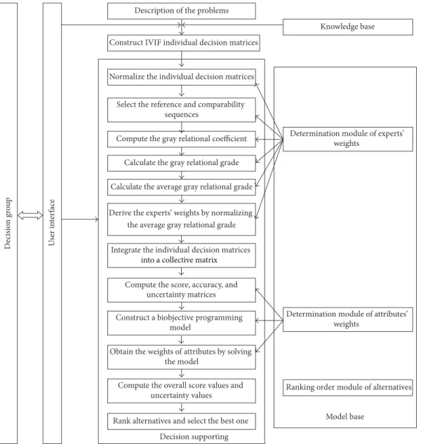
increases, the procedure solving a MAGDM may be compli-cated. In this case, a decision supporting system (DSS), which is a class of computer-based information system includ-ing knowledge-based systems [39, 40], can be formulated to help experts improve their decision-making level and quality through problem analysis, establishment of models, and simulation of decision-making process in a human-computer interaction way.Figure 1depicts a framework of DSS designed in this paper for MAGDM with IVIFSs.

As shown inFigure 1, the DSS consists of three modules: User interface, Knowledge base and Model base. Gener-ally, the user interface establishes an interaction between experts and inputs the basic decision information, such as attributes, alternatives and assessment values of alternatives on attributes. The main function of Knowledge base is to help experts perform information transformation and store the corresponding information. For example, the ratings of alternatives on attributes given by experts are transformed

(7)

D ecisio n gr o u p U ser in te rface

Description of the problems

Construct IVIF individual decision matrices

Normalize the individual decision matrices

Select the reference and comparability sequences

Compute the gray relational coefficient Calculate the gray relational grade Calculate the average gray relational grade

Derive the experts’ weights by normalizing the average gray relational grade

Compute the score, accuracy, and uncertainty matrices Construct a biobjective programming

model

Obtain the weights of attributes by solving the model

Compute the overall score values and uncertainty values

Rank alternatives and select the best one

Knowledge base

Decision supporting

Determination module of experts’ weights

Determination module of attributes’ weights

Ranking order module of alternatives

Model base Integrate the individual decision matrices

into a collective matrix

Figure 1: Framework of interval-valued intuitionistic fuzzy MAGDM decision supporting system.

into IVIF forms from which individual decision matrices with IVIFSs are constructed and used for the next calculation pro-cedure. Model base involves the methods, such as extended GRA and objective programming as mentioned above. Thus, the ranking of alternatives can be deduced and the optimal decision can be derived by DSS.

4. A Cloud Service Selection Problem and

Comparison Analysis

In this section, a real cloud service selection problem is given to illustrate the application of the proposed method. Meanwhile, the comparison analysis is also conducted to show the superiority of the proposed method.

4.1. A Cloud Service Provider Selection Problem and the

Solution Process. Due to the limited technology and capital,

an enterprise itself may be unable to build the cloud platform and tries to seek a cloud service to realize its CRM. After

the market research and preliminary screening, there are four potential cloud services for further evaluation, including SAP Sales on Demand (𝐴₁), Salesforce Sales Cloud (𝐴₂), Microsoft Dynamic CRM (𝐴₃) and Oracle Cloud CRM (𝐴4). Four experts (𝑒1, 𝑒2, 𝑒3, 𝑒4) are invited to evaluate

these cloud services on five indicators (attributes), including performance (𝑢1), payment (𝑢2), reputation (𝑢3), scalability

(𝑢₄), and security (𝑢₅). In terms of each attribute, each expert has presented his (her) normalized evaluation information for four cloud services in Tables1–4.

The preference relation set of attributes information supplied by experts is as follows:

𝐷 ={_{ { 𝜔₁≤2𝜔₂; 0.05≤ 𝜔₂− 𝜔₄≤0.1; 𝜔₅≥2𝜔₃; 𝜔₁ ≤0.4; 𝜔₁+ 𝜔₂+ 𝜔₃≥0.3; ∑𝑛 𝑗=1 𝜔_𝑗=1; 𝜔_𝑗≥0}_} } . (30)

(8)

Table 1: IVIF decision matrixR₁. 𝑢₁ 𝑢₂ 𝑢₃ 𝑢₄ 𝑢₅ 𝐴₁ (_[[0.55, 0.65], 0.15, 0.25]) ([0.35, 0.55], [0.35, 0.45]) ([0.65, 0.75], [0.15, 0.25]) ([0.55, 0.75], [0.05, 0.15]) ([0.10, 0.40], [0.30, 0.50]) 𝐴₂ (_[[0.35, 0.45], 0.25, 0.35]) ([0.15, 0.35], [0.15, 0.35]) ([0.35, 0.45], [0.45, 0.55]) ([0.25, 0.45], [0.45, 0.55]) ([0.70, 0.80], [0.10, 0.20]) 𝐴₃ (_[[0.55, 0.65], 0.15, 0.25]) ([0.75, 0.85], [0.05, 0.15]) ([0.55, 0.85], [0.15, 0.15]) ([0.45, 0.65], [0.25, 0.35]) ([0.50, 0.60], [0.20, 0.30]) 𝐴₄ (_[[0.35, 0.55], 0.35, 0.45]) ([0.15, 0.25], [0.65, 0.75]) ([0.15, 0.25], [0.55, 0.75]) ([0.35, 0.45], [0.35, 0.55]) ([0.20, 0.30], [0.50, 0.60]) Table 2: IVIF decision matrixR₂.

𝑢1 𝑢2 𝑢3 𝑢4 𝑢5

𝐴1 (_[[_{0.25, 0.45}0.45, 0.55_]]₎, (_[[_{0.40, 0.60}0.30, 0.40_]]₎, (_[[_{0.10, 0.15}0.55, 0.65_]₎], (_[[_{0.05, 0.25}0.55, 0.65_]]₎, (_[[_{0.25, 0.45}0.15, 0.35_]]₎, 𝐴2 (_[[_{0.30, 0.40}0.35, 0.55_]]₎, (_[[_{0.30, 0.70}0.10, 0.30_]]₎, (_[[_{0.35, 0.45}0.25, 0.35_]]₎, (_[[_{0.55, 0.65}0.25, 0.35_]]₎, (_[[_{0.05, 0.15}0.65, 0.85_]]₎, 𝐴3 (_[[_{0.25, 0.35}0.45, 0.65_]]₎, (_[[_{0.10, 0.20}0.60, 0.80_]]₎, (_[[_{0.05, 0.15}0.65, 0.75_]₎], (_[[_{0.25, 0.35}0.45, 0.65_]]₎, (_[[_{0.15, 0.35}0.55, 0.65_]]₎, 𝐴4 (_[[_{0.35, 0.55}0.35, 0.45_]]₎, _[([_{0.60, 0.80}0.10, 0.20_]]₎, (_[[_{0.65, 0.75}0.05, 0.15_]]₎, (_[[_{0.35, 0.55}0.35, 0.45_]]₎, (_[[_{0.45, 0.55}0.25, 0.45_]]₎,

Step 1. See Tables1–4.

Step 2. Calculate the weights of experts.

We take the weights of experts on𝑢₁as an example, that is,𝜆𝑘₁ (𝑘 = 1,2,3,4), to illustrate the calculating process of the experts’ weights. The calculating processes for𝜆𝑘₁are as follows:

(i) Select the reference sequence and comparability sequences.

Selecting ̃r1₁ as a reference sequence and ̃r2₁, ̃r3₁, ̃r4₁ as comparability sequences, where

̃ r1₁= (̃𝑟₁₁1, ̃𝑟1₂₁, ̃𝑟₃₁1, ̃𝑟1₄₁) = (([0.55,0.65] , [0.15,0.25]) , ([0.35,0.45] , [0.25,0.35]) , ([0.55,0.65] , [0.15,0.25]) , ([0.35,0.55] , [0.35,0.45])) ; ̃ r2₁= (̃𝑟₁₁2, ̃𝑟2₂₁, ̃𝑟₃₁2, ̃𝑟2₄₁) = (([0.45,0.55] , [0.25,0.45]) , ([0.35,0.55] , [0.30,0.40]) , ([0.45,0.65] , [0.25,0.35]) , ([0.35,0.45] , [0.35,0.55])) ; ̃ r3₁= (̃𝑟₁₁3, ̃𝑟3₂₁, ̃𝑟₃₁3, ̃𝑟3₄₁) = (([0.45,0.75] , [0.15,0.25]) , ([0.45,0.55] , [0.25,0.45]) , ([0.25,0.45] , [0.35,0.45]) , ([0.35,0.45] , [0.25,0.45])) ; ̃ r4 1= (̃𝑟114, ̃𝑟214, ̃𝑟314, ̃𝑟441) = (([0.65,0.75] , [0.15,0.25]) , ([0.40,0.50] , [0.40,0.50]) , ([0.40, 0.50] , [0.30, 0.40]) , ([0.30, 0.40] , [0.40, 0.50])) . (31) (ii) Compute the gray relational coefficient matrix. By (14)-(15), the gray relational coefficient matrix is derived as 𝜉1₁= ( 0.7122 1.000 0.8739 0.9489 0.9489 0.8739 0.5115 0.9489 0.9489 0.7766 0.6645 0.8739 ) . (32)

(iii) Calculate the gray relational grades. According to(16), we have 𝜂 (̃r2₁, ̃r1₁) =1 4 4 ∑ 𝑖=1𝜉 21 𝑖1 =0.8837, 𝜂 (̃r3₁, ̃r1₁) =1 4 4 ∑ 𝑖=1𝜉 31 𝑖1 =0.8208, 𝜂 (̃r4₁, ̃r1₁) =1 4 4 ∑ 𝑖=1𝜉 41 𝑖1 =0.8160. (33)

(9)

Table 3: IVIF decision matrixR₃. 𝑢₁ 𝑢₂ 𝑢₃ 𝑢₄ 𝑢₅ 𝐴₁ (_[[0.45, 0.75], 0.15, 0.25]) ([0.35, 0.55], [0.25, 0.35]) ([0.60, 0.70], [0.10, 0.20]) ([0.55, 0.65], [0.05, 0.25]) ([0.35, 0.55], [0.25, 0.45]) 𝐴₂ (_[[0.45, 0.55], 0.25, 0.45]) ([0.25, 0.45], [0.35, 0.45]) ([0.40, 0.50], [0.30, 0.40]) ([0.15, 0.25], [0.65, 0.75]) ([0.65, 0.75], [0.15, 0.25]) 𝐴₃ (_[[0.25, 0.45], 0.35, 0.45]) ([0.65, 0.85], [0.05, 0.15]) ([0.50, 0.70], [0.10, 0.30]) ([0.55, 0.75], [0.15, 0.25]) ([0.65, 0.85], [0.05, 0.15]) 𝐴₄ (_[[0.35, 0.45], 0.25, 0.45]) ([0.15, 0.25], [0.55, 0.75]) ([0.10, 0.30], [0.50, 0.70]) ([0.25, 0.35], [0.45, 0.65]) ([0.15, 0.25], [0.55, 0.75]) Table 4: IVIF decision matrixR₄.

𝑢1 𝑢2 𝑢3 𝑢4 𝑢5

𝐴1 (_[[_{0.15, 0.25}0.65, 0.75_]]₎, (_[[_{0.30, 0.40}0.30, 0.40_]]₎, (_[[_{0.05, 0.15}0.75, 0.85_]₎], (_[[_{0.10, 0.30}0.50, 0.60_]₎], (_[[_{0.45, 0.65}0.15, 0.25_]]₎, 𝐴2 (_[[_{0.40, 0.50}0.40, 0.50_]]₎, (_[[_{0.20, 0.30}0.10, 0.20_]]₎, (_[[_{0.45, 0.55}0.35, 0.45_]]₎, (_[[_{0.40, 0.60}0.20, 0.30_]]₎, (_[[_{0.05, 0.15}0.65, 0.75_]]₎, 𝐴3 (_[[_{0.30, 0.40}0.40, 0.50_]]₎, (_[[_{0.10, 0.30}0.60, 0.70_]]₎, (_[[_{0.15, 0.15}0.55, 0.85_]₎], (_[[_{0.20, 0.30}0.40, 0.50_]]₎, (_[[_{0.25, 0.35}0.55, 0.65_]]₎, 𝐴4 (_[[_{0.40, 0.50}0.30, 0.40_]]₎, (_[[_{0.60, 0.70}0.10, 0.30_]]₎, (_[[_{0.55, 0.75}0.15, 0.25_]]₎, (_[[_{0.40, 0.50}0.20, 0.30_]]₎, (_[[_{0.45, 0.55}0.35, 0.45_]]₎,

By using(17), the average relational grade between expert 𝑒₁and all other three experts is obtained as

𝜂1₁= 1 3 𝑡 ∑ 𝑙=2 𝜂 (̃𝑟₁𝑙, ̃𝑟1₁) =0.8402. (34) Similarly, we can get

𝜂₁2=0.7754, 𝜂₁3=0.8319, 𝜂₁4=0.7664.

(35)

By employing (18), the weights of four experts with respect to𝑢₁are derived as:

𝜆1₁=0.2614, 𝜆2₁=0.2413, 𝜆3₁=0.2588, 𝜆4₁=0.2385.

(36)

The calculating processes for the weights of experts with respect to other attributes are omitted, and the results are shown inTable 5.

Step 3. Integrate individual decision matrices R_𝑘 (𝑘 =

1,2,3,4)into a collective decision matrixR= (̃𝑟_𝑖𝑗)_𝑚×𝑛by(19), that is, R = ( ([0.531,0.685] , [0.170,0.288]) ([0.326,0.482] , [0.320,0.440]) ([0.639,0.743] , [0.093,0.182]) ([0.535,0.663] , [0.062,0.234]) ([0.176,0.381] , [0.308,0.511]) ([0.389,0.514] , [0.292,0.420]) ([0.153,0.332] , [0.236,0.425]) ([0.339,0.439] , [0.375,0.476]) ([0.214,0.341] , [0.482,0.628]) ([0.665,0.796] , [0.074,0.178]) ([0.423,0.572] , [0.249,0.353]) ([0.658,0.809] , [0.070,0.191]) ([0.568,0.790] , [0.099,0.182]) ([0.459,0.636] , [0.209,0.310]) ([0.556,0.687] , [0.154,0.289]) ([0.338,0.467] , [0.331,0.484]) ([0.126,0.251] , [0.599,0.749]) ([0.109,0.239] , [0.561,0.736]) ([0.284,0.385] , [0.385,0.553]) ([0.249,0.378] , [0.480,0.595]) ) . (37)

Step 4. Derive the score matrix, accuracy matrix and

uncer-tainty matrix.

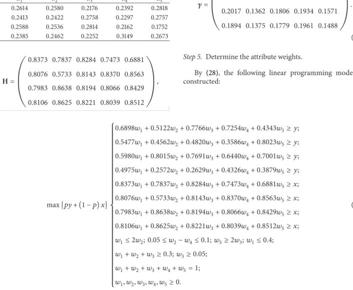
By(5),(7)and(8), the score matrix, accuracy matrix and uncertainty matrix of the collective matrixR are computed as: S∗= ( 0.6898 0.5122 0.7766 0.7254 0.4343 0.5477 0.4562 0.4820 0.3586 0.8023 0.5980 0.8015 0.7691 0.6440 0.7001 0.4975 0.2572 0.2629 0.4326 0.3879 ) ,

(10)

Table 5: The weights of each expert with respect to different attributes. 𝑢1 𝑢2 𝑢3 𝑢4 𝑢5 𝑒1 0.2614 0.2580 0.2176 0.2392 0.2818 𝑒2 0.2413 0.2422 0.2758 0.2297 0.2757 𝑒₃ 0.2588 0.2536 0.2814 0.2162 0.1752 𝑒4 0.2385 0.2462 0.2252 0.3149 0.2673 H= ( ( 0.8373 0.7837 0.8284 0.7473 0.6881 0.8076 0.5733 0.8143 0.8370 0.8563 0.7983 0.8638 0.8194 0.8066 0.8429 0.8106 0.8625 0.8221 0.8039 0.8512 ) ) , 𝛾 = ( ( 0.1625 0.2163 0.1716 0.2527 0.3119 0.1924 0.4267 0.1857 0.1630 0.1437 0.2017 0.1362 0.1806 0.1934 0.1571 0.1894 0.1375 0.1779 0.1961 0.1488 ) ) . (38)

Step 5. Determine the attribute weights.

By (28), the following linear programming model is constructed: max{𝑝𝑦 + (1− 𝑝) 𝑥} { { { { { { { { { { { { { { { { { { { { { { { { { { { { { { { { { { { { { { { { { { { { { { { { { { { { { { { { { { { { { { { { { { { 0.6898𝑤₁+0.5122𝑤₂+0.7766𝑤₃+0.7254𝑤₄+0.4343𝑤₅≥ 𝑦; 0.5477𝑤₁+0.4562𝑤₂+0.4820𝑤₃+0.3586𝑤₄+0.8023𝑤₅≥ 𝑦; 0.5980𝑤₁+0.8015𝑤₂+0.7691𝑤₃+0.6440𝑤₄+0.7001𝑤₅≥ 𝑦; 0.4975𝑤₁+0.2572𝑤₂+0.2629𝑤₃+0.4326𝑤₄+0.3879𝑤₅≥ 𝑦; 0.8373𝑤₁+0.7837𝑤₂+0.8284𝑤₃+0.7473𝑤₄+0.6881𝑤₅≥ 𝑥; 0.8076𝑤₁+0.5733𝑤₂+0.8143𝑤₃+0.8370𝑤₄+0.8563𝑤₅≥ 𝑥; 0.7983𝑤₁+0.8638𝑤₂+0.8194𝑤₃+0.8066𝑤₄+0.8429𝑤₅≥ 𝑥; 0.8106𝑤₁+0.8625𝑤₂+0.8221𝑤₃+0.8039𝑤₄+0.8512𝑤₅≥ 𝑥; 𝑤₁≤2𝑤₂; 0.05≤ 𝑤₂− 𝑤₄≤0.1;𝑤₅≥2𝑤₃; 𝑤₁≤0.4; 𝑤₁+ 𝑤₂+ 𝑤₃≥0.3;𝑤₃≥0.05; 𝑤₁+ 𝑤₂+ 𝑤₃+ 𝑤₄+ 𝑤₅=1; 𝑤₁, 𝑤₂, 𝑤₃, 𝑤₄, 𝑤₅≥0. (39)

Set𝑝 =0.5 and solve(39)with Simplex Method. The main components for(39)are as follows:

𝑦 =0.405, 𝑥 =0.779, 𝑤₁=0.3822, 𝑤₂=0.1911, 𝑤₃=0.05, 𝑤₄=0.1411, 𝑤₅=0.2355. (40)

Step 6. Compute the overall score and overall uncertainties

of each alternative.

Utilizing(22)and(24), we can calculate the overall scores and uncertainties of all alternatives which are shown in

Table 6.

Step 7. Rank alternatives in term ofDefinition 7. The result of

ranking is also listed inTable 6.

From Table 6, it can be seen that alternative 𝐴₃ is the best one, that is, Microsoft Dynamic CRM is the best cloud service.

4.2. Sensitivity Analysis for Parameter𝑝. In above example,

we get the computation results by a given a priori (𝑝 = 0.5). However, the attribute weights may vary as the value of weighting coefficient𝑝changes, which may result in different decision results. Hence, it is necessary to do the sensitivity analysis for parameter𝑝. The results of sensitivity analysis are depicted inFigure 2.

As shown in Figure 2, when the value of parameter 𝑝 changes from 0 and 1, although the overall scores of four providers change slightly, the rankings among the four cloud services remain unchanged.𝐴₃ is first, followed by𝐴₁ and followed by𝐴₂ and the𝐴₄ is ranked in the last all along. Therefore, we can use(29)freely.

(11)

Table 6: The overall scores, accuracies, and ranking of alternatives.

Alternative Score Uncertainty Ranking

𝐴1 0.6050 0.2213 2 𝐴₂ 0.5602 0.2213 3 𝐴3 0.6759 0.1765 1 𝐴4 0.4048 0.1704 4 0 0.1 0.2 0.3 0.4 0.5 0.6 0.7 0.8 0.9 1 0.35 0.4 0.45 0.5 0.55 0.6 0.65 0.7 p The s co res o f al te rn at iv es A1 A2 A3 A4

Figure 2: The overall scores of four candidate providers with respect to𝑝.

4.3. Comparison Analysis with the Method Using the Score

Function Given by Xu [30]. In the above cloud service

selection example, if the scores of alternatives are computed with the score function given by Xu [30] (see(4)), then the score matrix is given as

S = ( 0.3795 0.0244 0.5532 0.4508 −0.1313 0.0954 −0.0876 −0.0361 −0.2828 0.6047 0.1959 0.6029 0.5382 0.2880 0.4002 −0.0050 −0.4856 −0.4742 −0.1349 −0.2241 ) . (41)

The accuracy matrix retains unchanged. Putting the score matrix S and accuracy matrix H into (29), we get the following programming model:

max{𝑝𝑦 + (1− 𝑝) 𝑥} { { { { { { { { { { { { { { { { { { { { { { { { { { { { { { { { { { { { { { { { { { { { { { { { { { { { { { { { { { { { { { { { { { { 0.3795𝑤₁+0.0244𝑤₂+0.5532𝑤₃+0.4508𝑤₄−0.1313𝑤₅≥ 𝑦; 0.0954𝑤₁−0.0876𝑤₂−0.0361𝑤₃−0.2828𝑤₄+0.6047𝑤₅≥ 𝑦; 0.1959𝑤1+0.6029𝑤2+0.5382𝑤3+0.2880𝑤4+0.4002𝑤5≥ 𝑦; −0.005𝑤1−0.4856𝑤2−0.4742𝑤3−0.1349𝑤4−0.2241𝑤5≥ 𝑦; 0.8373𝑤1+0.7837𝑤2+0.8284𝑤3+0.7473𝑤4+0.6881𝑤5≥ 𝑥; 0.8076𝑤₁+0.5733𝑤₂+0.8143𝑤₃+0.8370𝑤₄+0.8563𝑤₅≥ 𝑥; 0.7983𝑤₁+0.8638𝑤₂+0.8194𝑤₃+0.8066𝑤₄+0.8429𝑤₅≥ 𝑥; 0.8106𝑤₁+0.8625𝑤₂+0.8221𝑤₃+0.8039𝑤₄+0.8512𝑤₅≥ 𝑥; 𝑤₁≤2𝑤₂; 0.05≤ 𝑤₂− 𝑤₄≤0.1;𝑤₅≥2𝑤₃; 𝑤₁≤0.4; 𝑤₁+ 𝑤₂+ 𝑤₃≥0.3;𝑤₃≥0.05; 𝑤₁+ 𝑤₂+ 𝑤₃+ 𝑤₄+ 𝑤₅=1; 𝑤₁, 𝑤₂, 𝑤₃, 𝑤₄, 𝑤₅≥0. (42)

Still let𝑝 = 0.5, by employing the Lingo Soft, we find that(42)has no feasible solution. Thus, the ranking order of alternatives cannot be obtained. This shows that introducing the normalized score function proposed in this paper is very important.

5. Conclusions

In order to stand out in the fierce competition, more and more enterprises begin to select cloud service as one of

their development strategy. Cloud service selection can be regarded as a kind of MAGDM. In this paper, we have studied the cloud service selection problems with IVIFSs and incom-plete information on attribute weights. A novel MAGDM method was proposed to solve this kind of GDM problems. There are following three dramatic features in the proposed method.

(1) The assessment values of alternatives on attributes are in the form of IVIFSs which can help experts express their preferences more flexibly.

(12)

(2) By extending the classical GRA method into IVIF environment, a new approach is presented to deter-mine the weights of experts. Furthermore, the weights of each expert obtained are different on different attributes, which is much closer to the real-world decision situation.

(3) A multiobjective programming model is constructed to derive the weights of attributes.

The future work of this study is to apply the proposed method to other management areas, such as risk investment, material selection and so on.

Conflict of Interests

The authors declare that there is no conflict of interests regarding the publication of this paper.

Acknowledgments

The authors would like to thank Associate Professor. Jiu-Ying Dong for improving the linguistic quality of this paper. This research was supported by the National Natural Science Foundation of China (nos. 71061006, 71161011, 61263018, 71361002 and 11461030), the National 863 Plan Project (2013AA12A402), the Humanities Social Science Programming Project of Ministry of Education of China (no. 09YGC630107), the Natural Science Foundation of Jiangxi Province of China (nos. 20114BAB201012 and 20142BAB201011), “Twelve five” Programming Project of Jiangxi province Social Science (2013) (no. 13GL17), the Natu-ral Science Foundation of Guangxi (GXNSF) (2013AA019349 and 2013AA278003), Science Foundation of Guangxi Edu-cational Committee (YB2014150) and the Excellent Young Academic Talent Support Program of Jiangxi University of Finance and Economics.

References

[1] L. Sun, H. Dong, F. K. Hussain, O. K. Hussain, and E. Chang, “Cloud service selection: state-of-the-art and future research directions,”Journal of Network and Computer Applications, vol. 45, pp. 134–150, 2014.

[2] S. Ding, C. Xia, Q. Cai, K. Zhou, and S. Yang, “QoS-aware resource matching and recommendation for cloud computing systems,”Applied Mathematics and Computation, vol. 247, no. 15, pp. 941–950, 2014.

[3] A. Goscinski and M. Brock, “Toward dynamic and attribute based publication, discovery and selection for cloud comput-ing,”Future Generation Computer Systems, vol. 26, no. 7, pp. 947–970, 2010.

[4] A. Jula, E. Sundararajan, and Z. Othman, “Cloud computing service composition: a systematic literature review,” Expert Systems with Applications, vol. 41, no. 8, pp. 3809–3824, 2014. [5] J. Siegel and J. Perdue, “Cloud services measures for global use:

the Service Measurement Index (SMI),” inProceedings of the Annual SRII Global Conference (SRII ’12), pp. 411–415, IEEE, San Jose, Calif, USA, July 2012.

[6] S. K. Garg, S. Versteeg, and R. Buyya, “SMICloud: a framework for comparing and ranking cloud services,” inProceedings of the

4th IEEE/ACM international conference on utility and Cloud on utility and Cloud computing (UCC’ 11), pp. 210–218, Melbourne, Australia, December 2011.

[7] M. Menzel, M. Sch¨onherr, and S. Tai, “(MC2)2: criteria, requirements and a software prototype for Cloud infrastructure decisions,”Software: Practice and Experience, vol. 43, no. 11, pp. 1283–1297, 2013.

[8] N. Limam and R. Boutaba, “Assessing software service quality and trustworthiness at selection time,”IEEE Transactions on Software Engineering, vol. 36, no. 4, pp. 559–574, 2010. [9] S. Silas, E. B. Rajsingh, and K. Ezra, “Efficient Service Selection

middleware using ELECTRE methodology for cloud environ-ments,”Information Technology Journal, vol. 11, no. 7, pp. 868– 875, 2012.

[10] P. Saripalli and G. Pingali, “MADMAC: multiple attribute decision methodology for Adoption of clouds,” inProceedings of the IEEE 4th International Conference on Cloud Computing (CLOUD ’11), pp. 316–323, Washington, DC, USA, July 2011. [11] L. Zhao, Y. Ren, M. Li, and K. Sakurai, “Flexible service

selection with user-specific QoS support in service-oriented architecture,”Journal of Network and Computer Applications, vol. 35, no. 3, pp. 962–973, 2012.

[12] C.-W. Chang, P. Liu, and J.-J. Wu, “Probability-based cloud storage providers selection algorithms with maximum avail-ability,” inProceedings of the 41st International Conference on Parallel Processing (ICPP ’12), pp. 199–208, Pittsburgh, Pa, USA, September 2012.

[13] S. Sundareswaran, A. Squicciarini, D. Lin, and S. Sun-dareswaran, “A brokerage-based approach for cloud service selection,” inProceedings of the IEEE 5th International Confer-ence on Cloud Computing (CLOUD ’12), pp. 558–565, Honolulu, Hawaii, USA, June 2012.

[14] Q. He, J. Han, Y. Yang, J. Grundy, and H. Jin, “QoS-driven service selection for multi-tenant SaaS,” inProceedings of the International Conference on Cloud Computing (CLOUD ’12), pp. 24–29, Honolulu, Hawaii, USA, June 2012.

[15] B. Martens, F. Teuteberg, and M. Gr¨auler, “Design and imple-mentation of a community platform for the evaluation and selection of Cloud computing services: a market analysis,” in Proceedings of the 19th European Conference on Information Systems (ECIS ’11), p. 215, Helsinki, Finland, June 2011. [16] J. Yang, W. M. Lin, and W. C. Dou, “An adaptive service selection

method for cross-cloud service composition,”Concurrency and Computation: Practice and Experience, vol. 25, no. 18, pp. 2435– 2454, 2013.

[17] G. L. Xu and F. Liu, “An approach to group decision making based on interval multiplicative and fuzzy preference relations by using projection,”Applied Mathematical Modelling, vol. 37, no. 6, pp. 3929–3943, 2013.

[18] S.-P. Wan and D.-F. Li, “Fuzzy LINMAP approach to hetero-geneous MADM considering comparisons of alternatives with hesitation degrees,”Omega, vol. 41, no. 6, pp. 925–940, 2013. [19] S.-P. Wan and J.-Y. Dong, “Possibility linear programming with

trapezoidal fuzzy numbers,”Applied Mathematical Modelling, vol. 38, no. 5-6, pp. 1660–1672, 2014.

[20] H. Akdag, T. Kalaycı, S. Karag¨oz, H. Z¨ulfikar, and D. Giz, “The evaluation of hospital service quality by fuzzy MCDM,”Applied Soft Computing, vol. 23, pp. 239–248, 2014.

[21] L. A. Zadeh, “Fuzzy sets,”Information and Computation, vol. 8, no. 3, pp. 338–353, 1965.

[22] K. T. Atanassov, “Intuitionistic fuzzy sets,” Fuzzy Sets and Systems, vol. 20, no. 1, pp. 87–96, 1986.

(13)

[23] K. Atanassov and G. Gargov, “Interval valued intuitionistic fuzzy sets,”Fuzzy Sets and Systems, vol. 31, no. 3, pp. 343–349, 1989.

[24] S.-P. Wan and J.-Y. Dong, “Power geometric operators of trape-zoidal intuitionistic fuzzy numbers and application to multi-attribute group decision making,”Applied Soft Computing, vol. 29, pp. 153–168, 2015.

[25] S. P. Wan, W. Feng, L. L. Lin, and J. Y. Dong, “An intuitionistic fuzzy linear programming method for logistics outsourcing provider selection,”Knowledge-Based Systems, vol. 82, pp. 80– 94, 2015.

[26] S. P. Wan and J. Y. Dong, “Interval-valued intuitionistic fuzzy mathematical programming method for hybrid multi-criteria group decision making with interval-valued intuitionistic fuzzy truth degrees,”Information Fusion, vol. 26, pp. 49–65, 2015. [27] S. P. Wan, G. L. Xu, F. Wan, and J. Y. Dong, “A new method for

Atanassov’s interval-valued intuitionistic fuzzy MAGDM with incomplete attribute weight information,”Information Sciences, vol. 316, pp. 329–347, 2015.

[28] S.-P. Wan and D.-F. Li, “Atanassov’s intuitionistic fuzzy pro-gramming method for heterogeneous multiattribute group decision making with atanassov’s intuitionistic fuzzy truth degrees,”IEEE Transactions on Fuzzy Systems, vol. 22, no. 2, pp. 300–312, 2014.

[29] J. L. Deng,Gray System Theory, Huazhong University of Science and Technology Press, Wuhan, China, 2002.

[30] Z.-S. Xu, “Methods for aggregating interval-valued intuitionis-tic fuzzy information and their application to decision making,” Control and Decision, vol. 22, no. 2, pp. 215–219, 2007 (Chinese). [31] G.-D. Li, D. Yamaguchi, and M. Nagai, “A grey-based decision-making approach to the supplier selection problem,” Mathemat-ical and Computer Modelling, vol. 46, no. 3-4, pp. 573–581, 2007. [32] W. J. Gu, Z. C. Sun, X. Z. Wei, and H. F. Dai, “A new method of accelerated life testing based on the Grey System Theory for a model-based lithium-ion battery life evaluation system,” Journal of Power Sources, vol. 267, pp. 366–379, 2014.

[33] H. B. Kuang, D. M. Kilgour, and K. W. Hipel, “Grey-based PROMETHEE II with application to evaluation of source water protection strategies,”Information Sciences, vol. 294, no. 10, pp. 376–389, 2015.

[34] F. Y. Meng, Q. Zhang, and X. H. Cheng, “Approaches to multiple-criteria group decision making based on interval-valued intuitionistic fuzzy Choquet integral with respect to the generalized𝜆-Shapley index,”Knowledge-Based Systems, vol. 37, pp. 237–249, 2013.

[35] S. Wan and J. Dong, “A possibility degree method for interval-valued intuitionistic fuzzy multi-attribute group decision mak-ing,”Journal of Computer and System Sciences, vol. 80, no. 1, pp. 237–256, 2014.

[36] Z. L. Yue and Y. Jia, “An application of soft computing technique in group decision making under interval-valued intuitionistic fuzzy environment,”Applied Soft Computing, vol. 13, no. 5, pp. 2490–2503, 2013.

[37] X. L. Zhang and Z. S. Xu, “Soft computing based on max-imizing consensus and fuzzy TOPSIS approach to interval-valued intuitionistic fuzzy group decision making,”Applied Soft Computing, vol. 26, pp. 42–56, 2015.

[38] D. F. Li, Multiobjective Many-Person Decision Makings and Games, National Defense Industry Press, Beijing, China, 2003.

[39] S. Cebi and C. Kahraman, “Developing a group decision support system based on fuzzy information axiom,” Knowledge-Based Systems, vol. 23, no. 1, pp. 3–16, 2010.

[40] G. Qian, H. Wang, and X. Q. Feng, “Generalized hesitant fuzzy sets and their application in decision support system,” Knowledge-Based Systems, vol. 37, pp. 357–365, 2013.

(14)

Submit your manuscripts at

http://www.hindawi.com

Hindawi Publishing Corporation

http://www.hindawi.com Volume 2014

Mathematics

Journal of

http://www.hindawi.com Volume 2014 Mathematical Problems in Engineering

Hindawi Publishing Corporation http://www.hindawi.com

Differential Equations International Journal of

Volume 2014

http://www.hindawi.com Volume 2014 Hindawi Publishing Corporationhttp://www.hindawi.com Volume 2014

http://www.hindawi.com Volume 2014 Mathematical PhysicsAdvances in

Complex Analysis

Journal of Hindawi Publishing Corporation

Optimization

Journal of

Combinatorics

http://www.hindawi.com Volume 2014 International Journal of Hindawi Publishing Corporation

Journal of

Function Spaces

Abstract and Applied Analysis Hindawi Publishing Corporation

http://www.hindawi.com Volume 2014 International Journal of Mathematics and Mathematical Sciences

Hindawi Publishing Corporation http://www.hindawi.com Volume 2014

The Scientific

World Journal

Discrete Dynamics in Nature and Society Hindawi Publishing Corporation

Discrete Mathematics

Journal of

http://www.hindawi.com Volume 2014 Hindawi Publishing Corporationhttp://www.hindawi.com Volume 2014

Stochastic Analysis

International Journal of