Effect of acceleration on quantum systems

Faculty of Mathematical, Physical and Natural Sciences Master studies in Physics

Degree Thesis

Effect of acceleration on

quantum systems

Academic Year 2007–2008

Supervisor

Prof. Rodolfo Figari

Candidate Nicola Vona matr. 358/47

Contents

Notation III

Introduction IV

1 First evidence 1

1.1 Uniformly accelerated observer . . . 1

1.2 Time dependent Doppler effect . . . 3

1.3 Field consequences . . . 4

1.4 Conclusion . . . 7

2 Quantum Fields and General Relativity 8 2.1 Quantum Theory of Scalar Field in Minkowski Spacetime . . 8

2.2 Quantum Theory of Scalar Field in Curved Spacetime . . . . 15

3 The Unruh effect 26 3.1 Minkowsi and Rindler particles . . . 26

3.2 Bogolubov transformations . . . 34

3.3 Thermalization theorem . . . 38

3.4 Physical interpretation . . . 42

3.5 Hawking effect . . . 44

4 Dynamical Casimir effect 50 4.1 Moving box . . . 51

4.2 Particles in a asymptotically stationary spacetime . . . 52

4.3 Wave equation for the field in the box . . . 53

4.4 Three remarkable cases . . . 57

4.4.1 Null acceleration . . . 57

4.4.2 Instantaneous acceleration . . . 58

4.4.3 Exponential acceleration . . . 58

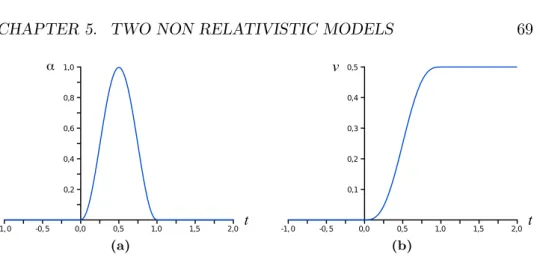
5 Two non relativistic models 60

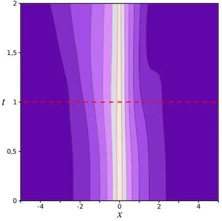
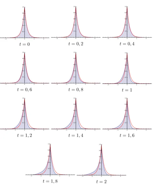
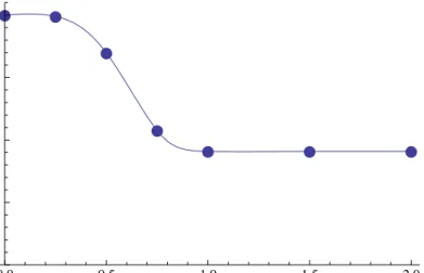
5.1 Harmonic oscillator . . . 60 5.2 Moving delta . . . 68 5.3 Conclusions . . . 73

Notation

The spacetime metric signature isn−2, wherenis the spacetime dimension. The metric determinant is indicated asg.

For tensors on spacetime is used abstract index notation, as in [20]. These indexes are identified with first letters of latin alphabet. Components in a particular frame are identified with greek letters; if spatial and temporal components are distinguished, the first ones are identified with central letters of latin alphabet and the second one with zero.

Units in which c = } = G = 1 are used, except that in the first and last

chapter.

Since the overtaking of Aristotelian theory, contrast between corpuscular and wave theory of light and matter has animated scientific debate. Newton and Huygens proposed for light the two descriptions in the XVII century; wave theory was established after Young diffraction experiment — 1801 — and was confirmed by Maxwell electromagnetism theory — 1864. The pho-toelectric effect — 1900 — proposed again the problem, suggesting that the combination of the two theories was necessary. For the matter the same contradiction came out at the early ’900, when some experiments seemed to support the wave theory (ex. Davisson and Germer experiment — 1927), while some others the corpuscular one (ex. Wilson’s observations with cloud chamber — 1911).

The Quantum Mechanics development solved for matter this paradoxical situation, describing the two aspects in a unified way. In particular Quantum Mechanics describes every system with a classical field that is propagated as a wave. Measurement previsions are evaluated from the field, so they will always have wave features. Applying the theory to a system made by a particle you have a description of this particle with both corpuscular and wave features.

Quantum Mechanics, in his first formulation, has two main problems. The first one is that it is not relativistic. Dirac dealt with this aspect in the ’20s. He tried to include in the quantum equation of evolution the rel-ativistic relation between energy and momentum. The resulting equation gives previsions in great agreement with experimental data, but it leads to some insurmountable contradictions, ex. non-positive probability distribu-tions. This theory can not be therefore interpreted as a quantum theory of relativistic particles. The second problem is that Quantum Mechanics describes light with classical electromagnetic field, that has wave features,

but not corpuscular ones.

These two problems are solved by Quantum Field Theory, developed in the ’50s.

Quantum Mechanics describes directly corpuscular features of micro-scopic systems. On the contrary in Quantum Field Theory there is not an obvious link between field and particles. This link must hence be defined separately, by a paradigm that specifies how extract information on parti-cles from the field. In the common formulation of the theory you solve the field equation in Fourier representation and quantize the resulting system of harmonic oscillators. So you are naturally taken to identify particles with quanta of oscillation (normal modes). This interpretation is supported by the fact that states with defined quanta number have defined energy pro-portional to the number and by the fact that you can construct a Fock space for field states (see chapter 2).

Fourier transform creates a link between particles and plane waves, that are positive frequency solutions of the field equation with respect to Min-kowski time. Plane waves viewed by a different inertial reference frame have a different frequency because of Doppler shift, but normal modes number is the same, so particle content of a state is the same for each inertial observer. The particle notion is therefore the same in each inertial frame, according to special relativity.

One plane wave viewed by a non-inertial reference frame, such as an uni-formly accelerated frame, becomes a superposition of plane waves because of time dependent Doppler shift. So passing from an inertial frame to a non-inertial frame the number of normal modes changes. This observation suggests that particle content of a field state is observer dependent. This result was obtained exactly by Fulling in 1973 [6]. He demonstrated that positive frequency functions with respect to Minkowski time defines an ac-ceptable particle definition because Minkowski spacetime is symmetric with respect to temporal translation. Therefore you have an acceptable particle definition for each set of functions that are positive frequency with respect to a timeτ if the spacetime is symmetric with respect to translations in the τ direction. Two particle definitions corresponding to two different temporal symmetries are in general different; this means that the vacuum state of one definition is not empty with respect to the other definition.

mathematical point of view, but in 1976 Unruh demonstrated that a particle detector moving along a trajectory with the proper timeτ detectsτ-particles instead of Minkowski-particles [18]. This shows that Fulling particles are not only a mathematical structure, but they are physically real. In the same work Unruh considers the particular case of Minkowski spacetime seen by an uniformly accelerated observer (Rindler spacetime). He showed that Minkowski vacuum, written in terms of accelerated particles, corresponds to a thermal state with temperature proportional to acceleration. Usually this situation is described asparticle creation from vacuum due to observer’s acceleration (Unruh effect).

The mentioned works are inserted in a wider sight, known as Quantum Field Theory in Curved Spacetime. This is the study of quantum fields when is present a gravitational field described by a curved spacetime, as in general relativity. In this sight the non-inertiality of a reference frame is expressed by an “apparent” gravitational field, that is a deviation of the metric from the Minkowski one. Studying the quantum field in a non-inertial frame is therefore equivalent to studying it when is present a fixed gravitational field. Historically the effect of acceleration on a quantum system was studied only in Quantum Field Theory because it involves particle creation. Never-theless you can’t think that acceleration has consequences only in relativistic conditions, on the contrary you can expect an effect similar to Unruh effect also in Non-Relativistic Quantum Mechanics. To see this effect you have to define an interpretative picture that accounts for particle creation. For example you can consider a system with a non-interacting particle “sea” in a bound state and you can interpret this state as the vacuum state. Particle creation is now the ionization of this state. In particular you can consider a system for which only the fundamental state is a bound state, while all the excited states are scattering states. In this case particle creation corresponds to spatial deconfinement. In this picture to the Unruh effect corresponds the system ionization due to acceleration.

The effect of acceleration in Quantum Field Theory is presented in this thesis. The same effect is considered in non relativistic conditions too, using two explicit models.

The thesis is structured as follows:

Chapter 1 A simplified derivation of the Unruh effect is presented. This derivation is based on time dependent Doppler effect and is not

rigor-ous, but is useful to underline the physical origin of the phenomenon.

Chapter 2 Quantum Field Theory in Curved Spacetime is presented as an extension of Quantum Field Theory in Minkowski spacetime. This theory provides the methods necessary to study the Unruh effect in a rigorous way.

Chapter 3 The theory established in chapter 2 is applied to the case of Minkowski spacetime, finding the connection between the particle def-inition of an inertial observer and of an accelerated observer. The vac-uum state of the inertial observer is then expressed as thermic state of the accelerated observer. Finally the analogy between Rindler and Schwarzschild metrics is used to present an analogy between Unruh effect and Hawking effect (black holes evaporation).

Chapter 4 A particular case of dynamical Casimir effect is addressed. In this case the field is confined in a box that undergoes a phase of acceler-ation. This configuration appears more realistic than the configuration considered in the Unruh effect, moreover is similar to the scattering problem, widely studied in physics.

Chapter 5 Two non-relativistic models are proposed to study the effect of the acceleration in these conditions. The first one is solved analytically, the second one numerically.

A first evidence of the

thermal effect of acceleration

Quantum Field Theory is developed on the basis of special relativity, so is expressed from the point of view of an inertial observer. How does the theory change for an accelerated observer?

To answer this question Quantum Field Theory in Curved Spacetime is necessary, but the development of this theory is quite difficult. In order to achieve an intuitive idea of the effect of acceleration, in this chapter a simplified analysis of the problem is presented [1]. This analysis is not rigorous, but is explanatory of the physical origin of the phenomenon.

1.1

Uniformly accelerated observer

Consider a flat spacetime with only one spatial dimension and an observer with constant speed in this spacetime. We will call this observer inertial or Minkowskian or M and we will denote his coordinates with{t, z}.

Consider another observer, called of Rindler or R, uniformly accelerated along the positive z axis of the inertial observer. Uniformly accelerated means that the observer has the same acceleration at every time with respect to the reference frame in which the observer is at rest in that moment. In this frame the acceleration isa= dv/dt0 >0, while the acceleration in the Minkowskian frame is given be the Lorentz transformation:

dv dt =a 1−v 2 c2 3/2 1

In order to obtain the speed of the R observer in the M frame you should integrate this equation withv(t= 0) = 0, but it is simpler to evaluate it in terms of the proper timeτ:

dv dt = dv dτ dτ dt = dv dτ 1− v 2 c2 1/2 ⇒ dv dτ =a 1−v 2 c2 ⇒v(τ) =ctanh aτ c

where it was used the relation dt= dτ /p1−v2_/c2_.

The R observer trajectory in the M frame is given by the integral of the equation:

dz dt =v(t)

but it is still simpler to consider this trajectory in terms of the proper time τ, given by: dt dτ = 1−v 2_(τ) c2 −1/2 dz dτ dτ dt =v(t(τ)) therefore dt dτ = cosh aτ c ⇒t(τ) = Z τ 0 cosh aτ0 c dτ0= c asinh aτ c dz dτ = csinh aτ c ⇒ z(τ) = c Z τ 0 sinh aτ0 c dτ0 = c 2 a cosh aτ c

Finally the trajectory of the R reference origin in the Minkowski frame, parametrized with the proper time, is:

     t(τ) = c asinh aτ c z(τ) = c 2 a cosh aτ c (1.1)

1.2

Time dependent Doppler effect

Consider a plane wave in the M frame, with wave vector~k//~ez and frequency

ωk=kc:

A(t, z) =A0eiϕ±(t,z) with ϕ±(t, z) =kz±ωkt

The observer in the origin of the M reference frame sees the wave A(t) = A0e±iωkt, while the observer in the origin of the R frame moves along the

trajectory (1.1) and sees the wave: A(τ) =A(t(τ), z(τ)) =A0 exp h iωk c a coshaτ c ±sinh aτ c i so A(τ) =A0 exp h ±iωkc a e ±aτ c i

Therefore the R observer doesn’t see a plane wave, but a superposition of plane waves (time dependent Doppler effect):

A(τ) =

Z ∞

−∞

dΩA(Ω)e e−iΩτ

where Ω is the frequency of R frame plane waves and (for waves moving toward−z) e A(Ω) = 1 2π Z ∞ −∞ dτ0A0 exp h ic aωke a cτ 0i eiΩτ0 Intensity of each plane wave seen by R is

|A(Ω)|e 2 = A2₀ (2π)2 Z ∞ −∞ dτ0 exp h ic aωke a cτ 0i eiΩτ0 2

Introducing the variabley=eaτ0/c _{in the integral we have}

Z ∞ −∞ dτ0 exp h ic aωke a cτ 0i eiΩτ0 = Z ∞ 0 eiacωky yi c aΩ c ay −1_dy= = c a Z ∞ 0 cosc_aωky+isin_acωky yicaΩ−1dy This integral converges only for 0 <Re i_acΩ <1, but can be regularized considering Ω →Ω−ia_cε, with 0 < ε <1, and taking the limit forε→ 0.

In such way we have Z ∞ −∞ dτ0 exp h ic aωke a cτ 0i eiΩτ0 = c_{a a}cωk −ic aΩ _e−π2 c aΩ Γ ic aΩ (1.2)

Using the relation|Γ(ix)|2 ₌ π

xsinh(πx) we obtain |A(Ω)|e 2 = cA2₀ 2πaΩ 1 e2πcaΩ−1

Time dependent Doppler effect therefore results in the Planck factor (e }

Ω

kB T −1)−1, typical of a Bose-Einstein distribution with temperature T =

}a

2πkBc, called Hawking-Unruh temperature. Note that this temperature is very small for experimental practicable accelerations: substituting the con-stants with their MKS numerical values we haveT = (4·10−21 s_m2K) a.

1.3

Field consequences

In the previous section we studied the case of a single plane wave (i.e. a single frequency), finding that in an accelerated frame it becomes a superposition of plane waves. When you quantize the scalar field you identify plane waves with single particle states, therefore Doppler effect turns a single particle state of the inertial frame into a superposition of single particle states of the accelerated frame.

Consider a massless real scalar field, in one dimension z, quantized in the whole space:

φ(t, z) = Z ∞ −∞ dk q }c2 2πωk ake−iωkt+a†−ke iωkt eikz with ωk=|kc| (1.3) The excitation energy operator of the field is

W = H−E0 = }

2π

Z ∞

−∞

dk ωkNk

whereN_k=a†_kakis the “field quantum number with momentumk” operator

The inertial observer in the origin sees the field φ(t) =φ(t, z= 0) = Z ∞ −∞ dk q }c2 2πωk ake−iωkt+a † −ke iωkt

The accelerated observer sees the field φ(τ) = φ(t(τ), z(τ)), obtained substituting (1.1) (page 2) in (1.3): φ(τ) = Z ∞ −∞ dk q }c2 2πωk ak exp h ic aωk(εke −εkaτc ) i + +a†_k exp h −ic aωk(εke −εkaτ_{c )} i

withεk= _|k_k| = signk. The number operator Np relative to this observer is

defined by Np = b†pbp, where bp operators come from the expansion of the

fieldφ(τ) with respect to the plane waves of the accelerated frame: φ(τ) = Z ∞ −∞ dp q }c2 2πΩp bpe−iΩpτ +b†−peiΩpτ

In order to find bp operators we consider the Fourier transform of the

fieldφ(τ): g(Ω) = 1 2π Z ∞ −∞ dτ φ(τ)eiΩτ φ(τ) = Z ∞ −∞ dΩ g(Ω)e−iΩτ = Z ∞ 0 dΩ g(Ω)e−iΩτ +g(−Ω)eiΩτ then bp= q πΩp 2} g(Ωp)

Suppose that the field is in the vacuum state of the inertial observer, denoted with|0i_M. The mean value ofN_p, quantum number with momentum koperator, in the accelerated frame is:

Mh0| Np|0iM = =_Mh0|b†_pbp|0iM = πΩp 2} Mh0|g †_(Ω p)g(Ωp)|0iM = = Ωp 8π} Z ∞ −∞ dτ Z ∞ −∞ dτ0 e−iΩpτ _eiΩpτ0 Mh0|φ †_(τ)φ(τ0_)|0i M = = Z ∞ −∞ dk c 2 8π Ωp ωk |I_k(Ωp)|2

with Ik(Ω) = Z ∞ −∞ dτ eiΩτ exp h −ic aωk(εke −εkaτ_{c )} i = = c a e −π 2 c aΩ c aωk iεkacΩ _{Γ −iε} k_acΩ

where we considered that just the term proportional to_Mh0|aka†_k0|0i_M =δ_kk0

gives a contribution and solved the integral as in (1.2). So we have Mh0| Np|0iM = c4 8πa2 e −πc_aΩp Z ∞ −∞ dk Ωp ωk Γ −iε_kacΩ_p 2

By the property Γ∗(z) = Γ(z∗), from which it follows that |Γ(i x)|2 = |Γ(−i x)|2, we have Mh0| Np|0iM = c3 4πa2 e −πc_aΩp _Ω p Γ ic aΩp 2 Z ∞ 0 dωk 1 ωk

The integral with respect to ωk diverges, so the accelerated observer

sees an infinite number of quanta with momentump in the field state|0i_M. Therefore let us calculate the fraction of excitation energy relative to the momentum pon the total excitation energy:

ep = Wp W = Mh0| Np|0iM Ωp R Mh0| Np|0iM Ωp dp/2π = 1 2π Z e −π_acΩp _Ω2 p Γ i_acΩ_p 2 where Z = 2 c Z ∞ 0 dΩ e−πacΩ Ω2 Γ i_acΩ 2

By the property |Γ(ix)|2₌ π

xsinh(πx) we have Z = 4πa c2 Z ∞ 0 dΩ Ω e2πacΩ−1 = πa 3 6c4 ep = 1 ZΩp 1 e2πacΩp₋₁ (1.4)

1.4

Conclusion

In this chapter it has been showed that plane waves of the inertial frame seen by an accelerated observer become superpositions of plane waves by virtue of time dependent Doppler effect. In quantum theory this means that single particle states of the two observers are different. In particular inertial vacuum state of the field for the accelerated observer is “full” of particles with the Bose-Einstein energy distribution (1.4), that has temperatureT =

}a

2πkBc, calledHawking-Unruh temperature. Proportionality between particle number spectrum and Bose-Einstein distribution is rigorously established by the so-calledthermalization theorem, that we will present in chapter 3.

Quantum Fields and

General Relativity

The previous chapter shows thatparticle content of a field state is observer dependent. In order to fully understand this statement you have to analyze the construction of Quantum Field Theory in an arbitrary spacetime (and therefore also with respect to an arbitrary observer).

In this chapter we introduce the fundamental ideas of the Quantum Field Theory in a Curved Spacetime [3, 21]. This theory studies quantum fields propagating in a classical gravitational field and has been developed to describe that phenomena for which both quantum and relativistic aspects are important, but for which the quantum nature of gravity is unessential and therefore negligible. In this case gravitation can be described by a classical curved spacetime, as prescribed by general relativity.

To study the Unruh effect we will consider only flat spacetime, but it is convenient that we start from the general case, coming back to the flat case in a second moment.

2.1

Quantum Theory of Scalar Field in Minkowski

Spacetime

In this section we review the Quantum Field Theory in Minkowski Spacetime pointing out its main steps. In this way we set up a “scheme” useful to generalize the theory.

Classical Klein-Gordon equation

Consider M, a n-dimensional Minkowski spacetime with metric ηµν with

positive signature and denote withx = (t, ~x) = (x0_{, ~x) its points. Consider}

a scalar fieldφ:M →_R, satisfying the Klein-Gordon equation1

−m2φ(x) = 0 (2.1)

where ≡ ηµν∂µ∂ν ≡ −∂02+

P

i∂i2. This equation cam be obtained from

the lagrangian density L(x) =−1 2 η µν_∂ µφ ∂νφ+m2φ2 = 1 2 ˙ φ2−(∇φ)~ 2−m2φ2 (2.2) with ˙φ=∂tφ, considering the action

S =

Z

M

L(x) dnx (2.3)

and demanding that δS = 0 for field variations null at initial and final instant.

We can consider the hamiltonian densityH, that is the Legendre trans-form ofL:

H =πφ˙−L π = ∂L ∂φ˙ whereπ is the canonical momentum density.

The system energy corresponds to the hamiltonian operator H = Z H(x) dn−1x In our case π = ˙φ H = 1 2 ˙ φ2+ (∇φ)~ 2_+m2_φ2 _(2.4)

Note that hamiltonian formalism distinguishes space and time, breaking the theory covariance. This means that with respect to an other reference frame π and H are different.

Equation (2.1) is linear, so its solution space is a vector space. Con-1_{If you consider the whole space then the boundary condition isφ −→}

|~x|→∞0 sufficiently

rapidly to have finite (2.5) norm; if you consider a box then the boundary condition is periodic.

sidering complex solutions too we are able to write down complete sets of solutions. Define on this space the scalar product

(φ1, φ2) = Z ¯ t φ1(x)(−i ↔ ∂t)φ∗2(x) dn−1x (2.5) where φ1(x)(−i ↔ ∂t)φ∗2(x)≡φ1(x) (−i∂_t)φ∗₂(x) − (−i∂_t)φ1(x) φ2(x)∗

and the integral is evaluated on the spacelike hyperplane of equationx0 = ¯t, with fixed ¯t. This product is independent of ¯tchoice2and has the properties:

(φ1, φ2)∗ = (φ2, φ1)

(αφ1, φ2) =α(φ1, φ2) (φ1, αφ2) =α∗(φ1, φ2)

(φ∗₁, φ2) =−(φ∗2, φ1) (φ1, φ∗2) =−(φ2, φ∗1)

(φ∗₁, φ∗₂) =−(φ2, φ1) =−(φ1, φ2)∗ (φ, φ∗) = 0

Consider the set of solutions such as 0 < (φ, φ) < ∞. On this set the product (2.5) defines a norm. Consider the Hilbert spaceHobtained by the completion of this set with respect to the norm only just defined. We call

orthonormal basis on this space a set of solutions{u_~k}_~k∈

Rn−1 such that

• {u_~k}_~k is a complete set ofH (even in generalized sense) • (u~_k, u~_k0) =δ(n−1)(~k−~k0), therefore (u∗_~ k, u ∗ ~_k0) =−δ (n−1)_(~k−~k0₎ • (u~_k, u_~∗_k0) = 0 ∀~k, ~k 0

The solutionsu~_k are also calledpositive frequency modes with respect to the

scalar product (2.5).

You can expand each solution ψ with respect to an orthonormal basis 2

Denote with Σ¯t the hyperplane of equation x0 = ¯t and with nµ its future

ori-ented normal versor (that is parallel tox0 axis). Therefore∂t = nµ∂µ and (φ1, φ2)t¯= R

Σ¯tφ1(x)(−i ↔

∂µ)φ∗2(x) dσµ.

Denote with V the volume between the two hyperplanes Σ¯t and Σ¯¯t, so (φ1, φ2)¯t−

(φ1, φ2)¯¯t = R ∂V φ1(x)(−i ↔ ∂µ)φ∗2(x) dσµ = R V∂ µ [φ1(x)(−i ↔ ∂µ)φ∗2(x)] dnx = 0 where we

used Gauss theorem and Klein-Gordon equation (if the field is confined into a box then

∂V includes also a timelike surface Σlthat has null-contribution to the integral by virtue

with the expression ψ(x) = Z dn−1~k a~_ku~_k(x) +b~_ku~∗_k(x) a~_k = (ψ, u~_k) b~_k=−(ψ, u∗~_k)

In particular, for a real solutionφ φ(x) = Z dn−1~k a_k~u~_k(x) +a~∗_ku ∗ ~ k(x)

One orthonormal basis is constituted by plane waves: u~_k(x) = √_2ω 1 ~ k(2π)n −1 e i~k·~x−iω~_kt _{where ω} ~ k = q |~k|2_+m2 _(2.6) Canonical Quantization

Canonical quantization is performed substituting the classical solution φ with an operator on the Hilbert spaceH, still denoted withφ, and imposing the equal time canonical commutation relations:

[φ(t, ~x), φ(t, ~x0)] = 0 [π(t, ~x), π(t, ~x0)] = 0 [φ(t, ~x), π(t, ~x0)] =iδ(n−1)(~x−~x0)

(2.7)

These commutation relations can be satisfied only if H has infinite dimen-sions.3 We use Heisenberg representation, so a system state is described by a vector in H. All physical quantities of the system are represented by self-adjoint operators onHand evolve according to the Heisenberg equation

˙

O =i[H, O]

where O is a self-adjoint operator that doesn’t explicitly depend on time.

Particles

So far the theory development has not involved any particle concept, that therefore is not a fundamental block of the theory, but rather a major in-terpretative key. To understand its importance is sufficient to consider that

3

If Hhas finite dimensions, therefore for each pair of operators TrAB = TrBA, so Tr [A, B] = 0, that is not compatible with (2.7).

experiments regarding Quantum Field Theory are usually called Particle Physics!

Let us introduce this important concept. Expand the fieldφwith respect to plane waves (2.6): φ(x) = Z dn−1~k a~_ku~_k(x) +a_~†_ku∗~_k(x) (2.8) Substituting this expansion into (2.7) we have

[a~_k, a~_k0] = 0 [a † ~_k, a † ~ k0] = 0 [a~_k, a † ~ k0] =δ n−1_(~k−~k0₎ (2.9)

These operators can be used to write H as a Fock space F. Consider the state|0i, calledvacuum, defined by the relation

a~_k|0i= 0 ∀~k

From vacuum we can construct thesingle particle states |1_~ki=a_~†

k|0i.

Sim-ilarly we can define the n~_k-particles states

|n_~ki= (a † ~_k) n~k p n~_k! |0i

where the multiplicative factor corresponds to the normalization hn_~k|n_~k0i=δn

−1_(~k−~k0

) (2.10)

For this states this relations are valid: a_~† k|n~ki= √ n+ 1 |(n+ 1)~_ki a~_k|n~_ki= √ n |(n−1)~_ki

Finally many particle states are

|n_~k 1, n~k2, . . . , n~kji= (a_~† k1) n~_k 1(a† ~_k2) n~_k 2· · ·(a† ~_kj) n~_kj (n~_k1!n~_k2!· · ·n~_k j!) 1/2 |0i

defined by N_~k =a†_~ ka~k N = Z dn−1~kN_~k in fact N_~k|n_~k 1, n~k2, . . . , n~kji= X i n~_ki δ(n−1)(~k−~ki) |n_~k 1, n~k2, . . . , n~kji N |n_~ k1, n~k2, . . . , n~kji= X i n~_ki |n_~ k1, n~k2, . . . , n~kji

Substituting the expansion (2.8) into (2.4) we find the energy expression in terms of operators a~_k: H = Z dn−1~k ω~k 2 a_~† ka~k+a~ka † ~_k = = Z dn−1~kN~_k+ 1 2δ (n−1)_(0)ω ~ k (2.11) Therefore H,N_~k = 0 H,N = 0 so states with defined number are energy eigenstates.

Increasing n~_k by one the energy of the state increases by ω~_k, therefore

we interpret n~_k as number of field quanta contained in the state and the

operators a_~†

k and a~k respectively as creation and annihilation operators of

one field quantum. The functions u~_k, used to define particles, are called

single particle solutions.

Energy regularization

From (2.11) we can see that the energy of any state with defined number is infinite, because of the divergent factor proportional to identity. This is the first of the large set of infinite quantities that appears in Quantum Field Theory. These quantities need to be regularized to gain physical significance. In our case regularization is very simple and takes advantage of the fact that energy is not absolutely measurable: what we measure are energy differences.

Mean energy of vacuum state is

E0 =h0|H|0i=δ(n−1)(0)

Z

dn−1~k ω~k 2

This quantity diverges because of two reasons: the factorδ(n−1)(0) and the integral ofω~_k. The first comes from quantization in the whole space and is

related to infiniteness of quantization volume. Indeed vacuum energy per unity of volume is [14] ε0= lim V→∞ E0 V = Z dn−1~k ω~k 2

The second reason of divergence is more relevant: it is the sum of zero point energy of each normal mode.

Regularization is made considering only excitation energy W, that is energy difference respect to vacuum energy:

W = H− h0|H|0i=

Z

dn−1~k N_~kω~_k

In a more formal wayW is defined by normal ordering: :a_~† ka~k :=a † ~_ka~_k :a~_ka † ~ k :=a † ~ ka~k W =: H : Summary

Elements used to develop quantum theory of scalar field in Minkowski space-time and its particle interpretation are:

1. Classical field dynamics: S and L 2. Space and time division: π and H

3. Time independent scalar product on solution space 4. Quantization: canonical commutation relations

5. Single particle solutions: orthonormal basis of classical solutions that define quantum states with defined energy

2.2

Quantum Theory of Scalar Field in Curved

Spacetime

In this section the construction of Quantum Field Theory in Curved Space-time is presented following the scheme drawn for quantization in Minkowski spacetime. We will see that there are some problems with the particle inter-pretation of the theory because particle concept is not always well-defined.

Spacetime structure

Let us suppose that spacetime:4

• is a differentiable metric manifoldM withndimensions and lorentzian metricgab. In this case you can identify three families of curves:

time-like (possible observer trajectories), light-time-like (light rays) and spacetime-like (linking events without any causal relation; on the contrary curves that are not spacelike are calledcausal curves)

• is such that classical Klein-Gordon equation has a unique solution if you assign initial condition on a suitable region

• is such that you can divide space and time in at least one manner (necessary to hamiltonian quantization)

Let us inspect the last two hypotheses, that are connected.

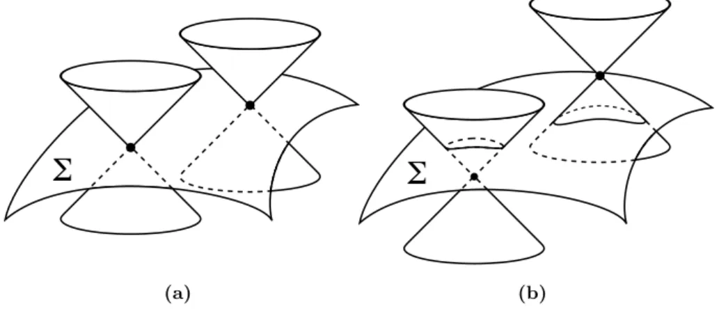
Firstly consider some definitions. A spacetime is said to be time ori-entable if for each event you can choice which half of light cone is the future and which is the past in a continuous way through the spacetime. A region Σ⊂M is said to be achronal if its points are not connectable by a timelike curve (see fig. 2.1a); we define domain of dependence of Σ the set D(Σ) of pointspofM such that every inextendible causal curve throughpintersects Σ (see fig. 2.1b). If D(Σ) = M, then Σ is said to be a Cauchy surface for M. It is possible to show that a Cauchy surface is a n−1 dimensional spacelike surface.5

A time orientable spacetime that admits a Cauchy surface is said to be

globally hyperbolic.

The following theorem holds: 4

For a construction of the theory under less strict conditions see for ex. [2, 13]

5

For a definition of extendibility of causal curves and a general treatment of causal structure of spacetime see [20]

�

(a)

�

(b)

Figure 2.1. (a) Causal cones of points belonging to an achronal surface don’t

intersect the same surface elsewhere. (b) All causal curves through points belonging to the domain of dependence of Σ intersect Σ.

Theorem [8, 5] If (M, gab) is globally hyperbolic, then exists a function

F :M →Rsuch that its level hypersurfaces Σt={x∈M :F(x) =t}

are Cauchy surfaces andM =S

t

Σt.

So if spacetime is globally hyperbolic then you can divide space and time, and therefore use hamiltonian formalism. Furthermore in this case causal curves intersect each surface Σt in one point, so you can reasonably expect

that classical dynamics is well defined if you assign initial data on surface Σt0. This is confirmed by:

Theorem [11] If (M, gab) is globally hyperbolic and you assign the functions

φ0 and ˙φ0 on a Cauchy surface Σt0, then there exists a unique solution φto Klein-Gordon covariant equation (2.14), defined on all ofM and such that φ|_Σ t₀ = φ0 and n a_∇ aφ|_Σt 0 = ˙φ0, where n a _{is the future}

oriented versor normal to Σt0. The solution φ varies continuously with the initial data. Moreover if you assign initial data only on a subsetσ⊂Σt0, then there exists a unique solutionφrestricted to the domain of dependence ofσ that depends only on initial data on σ. An analogous theorem holds for Green equation related to Klein-Gordon covariant equation. In the following we will always consider globally hyper-bolic spacetimes.

Let us set a last hypothesis: metric is assigned and not dependent on field, therefore we are studying scalar field dynamics in a gravitational frame,

disregarding the influence of scalar field on gravitational field. This influence is very important in astrophysics [21] and is related to quantization in general relativity; we will return on this aspect later (see page 22).

Klein-Gordon covariant equation

Let us extend the action (2.2)-(2.3) to a generic spacetime. Properties re-quested to action S =R

ML(x) d

n_{x are:}

• S is a real functional and has at least one extreme (so dynamics can come from action principle)

• L is a local function

• L depends only on the field and its first derivatives (so dynamics is determined by initial value of the field and its first derivatives) • If spacetime is flat, then S is invariant under Poincar`e transformations • S is covariant, that is not depending on coordinate system (so field

theory is compatible with general relativity) • S has the same symmetries of field

From this requirements you can extract, for the scalar field, a prescription [14] that allows to achieve a covariant action S from a Minkowski spacetime action S0, such that S = S0 ifgab=ηab:

• Substitutegab toηab

• Substitute covariant derivative∇_µto partial derivatives∂µ(when

ap-plied to scalar field they are equal)

• Substitute invariant volume element√−gdn_{xto volume element dtd}n−1_~x

• Add a term proportional to curvature andφ2

Applying this procedure to action (2.2)-(2.3) we have: S =−1 2 Z M gab∇_aφ∇_bφ+m2φ2+ζRφ2 √−gdnx (2.12)

whereRis the scalar curvature andζ is the coupling constant between field and curvature. The most common values ofζ areζ = 0, calledminimal cou-pling, andζ = 1₄ n_n−₋2₁, calledconformal coupling. In the conformal coupling case, if mass is zero, S is invariant under conformal transformations [7].

Through the expression S =R

ML(x) d

n_{xwe define the lagrangian}

den-sity L =− √ −g 2 gab∇_aφ∇_bφ+m2φ2+ζRφ2 (2.13) from which we have the equation of motion

−m2−ζR(x) φ(x) = 0 (2.14) where6 φ=gµν∇µ∇νφ= √1_−g∂µ( √ −g gµν_∂ νφ).

Note that also in this case equation of motion is linear with respect to φ(cf. (2.1)).

Hamiltonian formalism: space and time division

Consider a function F :M → R, such that spacetime can be written as a

collection of its level hypersurfaces Σt, with tas parameter, as seen on page

16 (in generalF choice is not unique). We can associate to this function a

vector field of time evolution ta, satisfying the equation ta∇aF = 1.

Introduce a coordinate system (t, xi_{), where t(x) = F(x) and x}i

co-ordinates on Σt, such that ta∇axi = 0. In this system (∂t)a = ta, so

˙

φ=∂0φ=∂tφ=ta∇aφ.

From (2.13) we have the canonical momentum density

π= ∂L ∂(∂0φ) =−√−g g0ν_∂ νφ=− √ −g ∂0_φ

therefore the hamiltonian density is H =π ∂0φ−L = √ −g 2 g iµ_∂ µφ∂iφ−g0µ∂µφ∂0φ+m2φ2+ζRφ2 = = √ −g 2 ∂iφ∂ i_φ−∂ 0φ∂0φ+m2φ2+ζRφ2 (2.15) Note thatπ andH depend on time choice, that isF choice, that in gen-6

It comes from∇µων =∂µων−1₂gρσωρ(∂µgνσ+∂νgµσ−∂σgµν), while ∇µf =∂µf,

eral is not unique. Therefore hamiltonian theory depends on chosen observer system.

We can make space and time division more explicit by considering apart directions that are orthogonal and tangential to space hypersurfaces Σt:

writetaasta=ta_⊥+t_//a =N na+t_//a, wherena= _k∇∇aaF_Fk is the future oriented versor normal to Σt. Denote with hab the riemannian metric induced bygab

on Σt, defined as the symmetric tensor that is null on vectors orthogonal to

Σtand works as gab on tangent vectors:

habna= 0 hab(δac +nanc) =gab(δac +nanc)

(+ sign in projector orthogonal tonacomes from the fact thatnais timelike, so it has negative norm) from which

hab =gab+nanb Substituting into (2.12) S = 1 2 Z M h (na∇aφ)2−hab∇aφ∇bφ−m2φ2−ζRφ2 i √ h Ndtdn−1x Fromta=N na+t_//a follows that

na∇_aφ= 1 N( ˙φ−t

a

//∇aφ)

Therefore lagrangian and canonical momentum densities are L = √ h 2 1 N( ˙φ−t a //∇aφ) 2_−N(hab_∇ aφ∇bφ+m2φ2+ζRφ2) π = ∂L ∂φ˙ = √ h 1 N( ˙φ−t a //∇aφ) = √ h na∇_aφ (2.16) Scalar product

Let us generalize the scalar product (2.5) with: (φ1, φ2) = Z Σ¯t φ1(x)(−i ↔ ∇a)φ∗2(x) dΣa= = Z Σ¯t φ1(x)(−i na ↔ ∇a)φ∗2(x) √ hdn−1x (2.17)

All properties stated for product (2.5) stand also for this one, except for the fact that now plane waves (2.6) are not, in general, solutions. Note that this product takes the same value if you choice differently both ¯tand space and time division.7

Canonical quantization

Canonical quantization is still performed substituting an operator on the Hilbert spaceHto the classical solutionφ, imposing the equal time canonical commutation relations(2.7) and using Heisenberg representation.

Particles

Particle definition that we adopt corresponds to the identification of particles andfield quanta. This means that we use as single particle solutions a basis {u_~k}whose operators a_~†

kand a~k satisfy commutation relations (2.9). These

relations are necessary to writeHas a Fock spaceF. Moreover Fock states must have definite energy.

Let us study what conditions come from requests put on solutions{u_~k}. Consider that {u_~k}_~k∈

R3 is a basis for H, therefore

φ(x) = Z dn−1~k a~_ku~_k(x) +a_~†_ku∗~_k(x) (2.18) Define a(u~_k) = (φ, u~_k) (2.19)

annihilation operator associated to the classical solution u~_k [12].

Consider a(u~_k), a(u~_k0) =(φ, u~_k),(φ, u~_k0) = =− Z Σt Z Σ_t0 φ(x)(ph(x)na(x) ↔ ∇_a)u_~∗ k(x) , φ(x0₎₍p_h(x0_)nb_(x0₎ ↔ ∇0_b)u∗_~ k0(x0) dn−1xdn−1x0 (2.20) Scalar product doesn’t depend on t, so we can set t0 =t. Using (2.16) we can recast (2.20) in terms of equal time canonical commutation relations

7

(2.7), from which follows that a(u~_k), a(u~_k0) = Z Σt u∗_~ k(x)(−i n a_∇↔ a)u~∗_k0(x) √ hdn−1x= (u_~∗ k, u~k0) By the substitutions u~_k→ −u∗~_k, u~_k0 → −u_~∗ k0 u~_k →u~_k, u~_k0 → −u_~∗ k0

we obtain also the commutators

a(u~_k)†, a(u~_k0)† = (φ,−u∗_~ k),(φ,−u ∗ ~ k0) = (u~_k, u~∗_k0) a(u~_k), a(u~_k0)† =(φ, u~_k),(φ,−u~∗_k0) = (u~_k0 , u~_k)

Summarizing, from classical solutions{u_~k} we have the annihilation op-eratorsa(u~_k) satisfying the commutation relations

a(u~_k), a(u~_k0) = (u∗_~ k, u~k0) a(u~_k)†, a(u~_k0)† = (u~_k, u∗~_k0) a(u~_k), a(u~_k0) † = (u~_k0, u~_k)

In order to obtain the commutation relations (2.9), necessary to writeH

as a Fock spaceF, we must therefore use as single particle solutions a basis of solutions that are orthonormal with respect to the product (2.17). In this casea~_k=a(u~_k) (cf. (2.18) and (2.19)).

The second request is that Fock states have defined energy. This means that hamiltonian operator H =R_Σ

tH d

n−1_{x commutes with number}

oper-atorN. Substituting the expansion (2.18) into (2.15) we obtain

H = Z dn−1~k Z dn−1~k0 (ReB~_k~k0)a † ~_ka~k0 + 1 2B~k~k0 δ (n−1)_(~k−~k0₎₊ +1 2A~k~k0 a~_ka~_k0 + 1 2A ∗ ~ k~k0 a † ~_ka † ~ k0 where A~_k~k0 = Z Σt √ −g gµi∂iu~_k∂µu~_k0−gµ0∂0u~_k∂µu~_k0 + (m2+ζR)u~_ku~_k0 dn−1x

B~_k~k0 = Z Σt √ −g gµi∂iu~_k∂µu~∗_k0−g µ0_∂ 0u~_k∂µu~∗_k0 + (m 2_+ζR)u ~ ku ∗ ~ k0 dn−1x In order to have [H,N] = 0 it must beA~_k~k0 = 0.

In Minkowski spacetime case we used plane waves as solutionsu~_k. Plane

waves are harmonic functions with respect to both time and space. In partic-ular time harmonicity is fundamental to write the hamiltonian as in (2.11), while you can think that spatial dependence is determined by Klein-Gordon equation, as a consequence of time dependance. Similarly we can expect that our requests are satisfied considering orthonormal solutions that are time harmonic. This expectation is validate if spacetime is stationary, i.e. it admits a timelike Killing 8 vector field ξa. Actually if you use the field ξaas vector fieldta of time evolution,9 then sufficient condition [21] so that solutions {u_~k} define single particle states satisfying our requests is that they are eigenfunctions of the operator ξa_∇

a=ta∇a=∂t:

∂tu~_k =−iω~_ku~_k con ω~_k≥0

This is a sufficient but not necessary condition, therefore in a generic spacetime there isn’t any preferred set of solutionsu~_k, so there isn’t an

obvi-ous particle definition. Only if spacetime is stationary there is a “natural” particle definition that come from time symmetry. Finally if there are more than one timelike Killing vectors, a different particle notion comes from each of them [6]. To each particle notion corresponds a different vacuum notion.10 This arbitrariness is the main feature of Quantum Field Theory in Curved Spacetime.

Energy regularization

Given the basis{u_~k} of single particle solutions, regularization can be per-formed as described on page 13. Naturally to different sets of functions u~_k

8

A vector fieldξais said to be a Killing vector field for the metricgabif it satisfies the

equation ξρ ∂ ∂xρgµν+gµρ ∂ξρ ∂xν +gρν ∂ξρ ∂xµ = 0 (2.21)

With respect to coordinates such thatξa= (∂x0)a, that isξρ=δρ₀, this equation becomes

∂

∂x0gµν = 0. Therefore metric doesn’t depend onx0, so system is symmetric for translation

along this coordinate. For further informations see [20].

9

In this casegabdoesn’t depend on time.

10_{Since we sett}a _{= ξ}a_{, different particle definitions can be seen as corresponding to}

correspond different notions of particle and vacuum, and so different regu-larizations. From the hypothesis that scalar field is not a source for gravita-tional field follows that only energy differences between different states are observable. On the contrary, to study gravity production by the field you use the semiclassical Einstein equation [21]

Gab= 8π hTabi

where Gab is the Einstein tensor and Tab is the energy-momentum tensor.

The tensor Tab is divergent and need to be regularized; the simplest

pro-cedure consists of postulating that vacuum state doesn’t give rise to grav-itational field and subtracting from hT_abi the mean value on vacuum Tab.

Now to different regularizations correspond different produced gravitational fields, with observable effects. Here starts a new chapter of Quantum Field Theory in Curved Spacetime, that we don’t discuss and that researches the “physical” vacuum, that is the vacuum that effectively produce no gravita-tional field, or researches a covariant regularization [21, 3, 7, 14].

Bogolubov transformations

We have seen that particle and vacuum definitions are not unique and de-pend on the choice of functions u~_k. So we can ask how two definitions

relative to two different sets {u_~

k} and {v~p} are linked.

11 _{Expand the field}

with respect to the two bases: φ(x) = Z dn−1~k a~_ku~_k(x) +a † ~_ku ∗ ~ k(x) = Z dn−1~p bp~v~p(x) +b † ~ pv ∗ ~ p(x) (2.22) We can also expand the functions v~p with respect to the u~_k and vice versa,

obtaining the Bogolubov transformations: u~_k= Z dn−1p~α~_{k ~p}v~p(x) +β~_{k ~p}v∗~p(x) (2.23) v~p = Z dn−1~k α_~∗ k ~pu~k(x)−β~k ~pu ∗ ~_k(x) (2.24) 11

These two sets are analogous to plane waves of Minkowski and Rindler considered on page 3 and the transformations that we are looking for are analogous to what considered on section 1.3.

with

α~_{k ~p} = (u~_k, vp~) = (v~p, u~_k)∗ β~_{k ~p} =−(u~_k, vp~∗) = (vp~, u∗~_k) (2.25)

Substituting (2.23) into (2.22) we get b~p= Z dn−1~k α~_{k ~p}a~_k+β~_{k ~}∗_pa † ~ k

while substituting (2.24) into (2.22) a~_k= Z dn−1~p α∗_~ k ~pb~p−β ∗ ~_{k ~p}b † ~ p

furthermore substituting (2.24) into (v~p, vp~0) =δn−1(~p−~p0) and into (v_~p, v∗

~

p0) =

0 we have the properties

Z dn−1~k α∗_~ k ~pα~k ~p0 −β~_{k ~p}β~_{k ~}∗_p0 =δn−1(~p−~p0) Z dn−1~kβ_{k ~}~_pα~_{k ~p}0 −α ∗ ~_{k ~p}β~_{k ~p}0 = 0

Operatorsa~_k andb~p lead to different Fock spaces, with different vacuum

states, defined by:

a~_k|0ia = 0 ∀~k b~p|0ib = 0 ∀~p Consider a~_k|0ib= Z dn−1~p α∗_~ k ~pb~p−β ∗ ~_{k ~p}b † ~ p |0i_b=− Z dn−1~p β_~∗ k ~p |1~pib from which bh0| N a ~ k |0ib= Z dn−1~p|β_{~k ~p}|2 (2.26)

If coefficients β~_{k ~p} are not zero, vacuum |0ib, obtained from functions v~p, can be not-annihilated by operators a~_k that correspond to functions u~_k;

moreover|0i_b contains a non-zero number of quanta of modes u~_k.

Similarly b~p|0ia = Z dn−1~k α~_{k ~p}a~_k+β~_{k ~}∗_pa † ~_k |0i_a= Z dn−1~k β_~∗ k ~p |1~kia

from which ah0| N b ~ p|0ia= Z dn−1~k|β_{~k ~p}|2 _(2.27)

The Unruh effect

We have seen that in a general spacetime particle and vacuum notions are not well defined. Only if spacetime is stationary there is a natural par-ticle definition, that rises from system symmetry. In this chapter we will reconsider the field quantization in Minkowski spacetime in light of the gen-eral theory developed in the previous chapter. We will see which particle definitions come from time symmetries of the system and what physical interpretation we can give them.

3.1

Minkowsi and Rindler particles

Let us derive a single particle states definition from the fact that spacetime is stationary, using the sufficient condition of page 22.

Minkowski particles

Consider the s+ 1 dimensional Minkowski spacetime and mark with {t, ~x} a global inertial reference frame, called M. With respect to this frame the metric is gµν =ηµν = −δµ0δ0ν+

P

iδµi δiν. A Killing vector field ξa satisfies

the equation (2.21) ξρ ∂ ∂xρgµν+gµρ ∂ξρ ∂xν +gρν ∂ξρ ∂xµ = 0 (3.1) 26

that with respect to coordinatesM is                ∂ξ0 ∂t = 0 ∂ξ0 ∂xi = ∂ξi ∂t ∂ξi ∂xj =− ∂ξj ∂xi (3.2)

The fields (∂µ)a satisfy this system, so they are Killing fields. This just

means that translations are isometries for Minkowski spacetime. Among this fields (∂t)a is timelike, so it can be employed to define a particle

no-tion. Using frame M we implicitly used (∂t)a as vector of time evolution,

therefore we have only to find solutions of Klein-Gordon1 equation that are eigenfunctions of (∂t)a. So this functions are such that

−∂_t2+X i ∂_i2−m2 u~_k= 0 ∂tu~_k=−iω~_ku~_k

This equations are satisfied by plane waves (2.6), so the prescription for the particle definition in a stationary spacetime applied to Minkowski space-time corresponds to the ordinary quantization, seen on section 2.1. Field expansion with respect to solutionsu~_k is

φ(x) = Z ds~k a~_ku~_k(x) +a † ~ ku ∗ ~ k(x)

while vacuum is defined by

a~_k|0iM = 0 ∀~k

1

Rindler particles

Translations are not the only isometries of Minkowski spacetime, for example Lorentz boosts are isometries too. A boost along thex direction is:

       t0 =γ (t−v x) x0 =γ (x−v t) y0 =y γ = √ 1 1−v2

where, to make notation simpler, first spatial coordinate (marked as x) is distinguished from the others (bold marked). Transformation is simpler if written in terms ofrapidity ν

(

t0 =tcoshν−xsinhν

x0 = −tsinhν+xcoshν with

(

γ = coshν

v γ = sinhν (3.3) For smallν we can truncate the transformation to the first order:

(

t0 =t−νx x0 =x−νt

the infinitesimal generator of this transformation is therefore the vector field ba=α

x(∂t)a+t(∂x)a

with constantα. This field satisfies the system (3.2), so it is a Killing field (obvious because it generates an isometry).

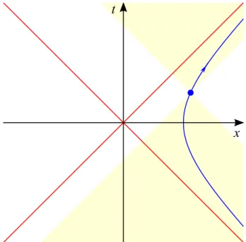
The ba norm is kbk2 _=ba_b a =gµνbµbν = −(b0)2+ X i bi2=α2(t2−x2)) and is timelike if|x|>|t|, so in regions I and II of fig. 3.1.

In order to construct a particle definition, as we have done with ∂t, we

need a timelike field on the whole spacetime. Nevertheless region I (or II) is globally hyperbolic and, even if not geodetically complete2, it can be treated

2

A set is said to be geodetically complete if all geodesics passing trough every point of the set are entirely comprised into the set. In general relativity it is understood that we refer to timelike and light-like geodesics, corresponding respectively to free particles and light rays, so completeness means that objects can’t “leave” the spacetime.

Regione I

Regione II

x

t

Figure 3.1

as a spacetime is its own right [7]. Therefore we can consider a quantum theory for region I (or II) alone, using ba as time evolution field (−ba _in

II because is future directed). Fock states we will obtain are said Rindler particles.

Region I: x∈(0,∞), t∈(−x, x).

Introduce the time function τ(t, ~x) such that

ba∇aτ = 1 that is x∂tτ +t∂xτ =

1 α

You can easily verify that this condition is satisfied by the function

τ(t, x) = 1 2αlog x+t x−t τ ∈(−∞,∞)

Level hypersurfaces of this function are Cauchy surfaces for the spacetime [21], so we can use τ as time function. The versor orthogonal to these surfaces isna= _kb_baa_k.

ξi(t, ~x)≡~ξ≡(ξ,υ) such that ba∇_aξi = 0 ∀i cio`e x∂tξi+t∂xξi= 0 (3.4) Consider therefore [14] ξ(t, x) =−1 α + p x2_−t2 _ξ∈− 1 α,∞ υ =y

Coordinates{τ, ξ,υ}are calledRindler coordinates3and are the coordinates of a reference composed by observers moving with uniform acceleration α [14]. In this frame line element is

ds2=−dt2+ d~x2=−(αξ+ 1)2dτ2+ d~ξ2 (3.5)

furthermorekbk2_{=−(αξ+ 1)}2_{, so}

ba∇a=∂τ na∇a=

1 (αξ+ 1)∂τ The scalar product (2.17) now is

(φ1, φ2) = Z ¯ τ dsξ φ~ 1(τ, ~ξ) _−i (αξ+ 1) ↔ ∂τ φ∗₂(τ, ~ξ) (3.6) In order to get to particle definition that derive from ba, we have to consider the solutions vI_~p of Klein-Gordon equation that are eigenfunctions ofba∇a: − 1 (αξ+ 1)2∂ 2 τ+ α (αξ+ 1)∂ξ+∂ 2 ξ+∂y2 −m2 v_~pI = 0 ba∇avI~p =−iΩ vp~I that is ∂τvI~p=−iΩ v~pI

3

Inverse transformations are (cf. (1.1))

t= αξ+ 1

α sinhατ x= αξ+ 1

Set4 vI_~p(τ, ~ξ) = p 1 2Ω(2π)s−1 e −iΩ τ+ip·y_ψI ~ p(ξ)

(now p~ stands for Ω > 0 and p ∈ Rs−1) so that eigenvalue equation is

satisfied, whileψI_~p(ξ) satisfies

(αξ+ 1)2 d 2 dξ2 +α(αξ+ 1) d dξ −(αξ+ 1) 2_m2 p+Ω2 ψ_~pI(ξ) = 0 (3.7)

wherem2_p =m2+p2. Imposing on vI_~p the normalization

(v_~pI, v_pI_~0) =δs−1(p−p0) δ(Ω−Ω0)

we find the normalization onψI_~p(ξ):

Z ∞ −1 α ψI Ω,p(ξ) ψΩI∗0_,p(ξ) (αξ+ 1) dξ=δ(Ω−Ω 0_{) (3.8)}

Introduce the variableζ = αξ_α+1, soζ ∈(0,∞) and equations (3.7) and (3.8) become ζ2 d 2 dζ2 +ζ d dζ −ζ 2_m2 p+ Ω2 α2 ˆ ψ_pI_~(ζ) = 0 (3.9) Z ∞ 0 ˆ ψ_Ω,I _p(ζ)ψˆ_ΩI∗0_,p(ζ) αζ dζ =δ(Ω−Ω 0_{) (3.10)}

where ˆψI_~p(ζ) =ψ_pI_~(ξ(ζ)). Equation (3.9) is a Bessel equation whose solutions,

normalized according to (3.10), are [6]

ˆ ψI_~p(ζ) = 1 π r 2Ω α sinh πΩ α KiΩ_α(mpζ)

whereK is the modified Bessel function [9]. Coming back to the variableξ:

ψ_~pI(ξ) = 1 π r 2Ω α sinh πΩ α KiΩ_α mp αξ+1 α

It can be proved that the set {vI

~ p, vI ∗ ~ p } is complete on region I [17]. 4

Note thatv~pI is a plane wave with respect toτ, circumstance that justifies what we

Region II: x∈(−∞,0), t∈(x,−x).

In order to have a future-oriented timelike vector consider −ba_{; time}

functionτ(t, ~x) now satisfies

−ba∇_aτ = 1 cio`e x∂tτ +t∂xτ =−

1 α Obviously this condition is satisfied by the function

τ(t, x) =− 1 2αlog x+t x−t τ ∈(−∞,∞)

Spatial coordinates still satisfy (3.4), but now set ξ(t, x) =−1 α − p x2_−t2 _{ξ ∈− ∞,−}1 α so that ξ > −1 α on regione I and ξ < − 1

α on region II. Now inverse

trans-formations are t= αξ+ 1 α sinh(−ατ) x= αξ+ 1 α cosh(−ατ) We have −ba∇a=∂τ na= −ba kba_k n a_∇ a= 1 (αξ+ 1)∂τ so the scalar product (2.17) is still expressed by (3.6).

Line element is still given by (3.5), so Klein-Gordon equation is the same as in region I; consider its solutionsvII_~p that are eigenfunctions of−ba_∇

a: − 1 (αξ+ 1)2∂ 2 τ+ α (αξ+ 1)∂ξ+∂ 2 ξ+∂2y−m2 v_~pII= 0 −ba∇av~pII=−iΩ vp~II that is ∂τvpII~ =iΩ vII~p

Therefore v_~pII(τ, ~ξ) = p 1 2Ω(2π)s−1 e iΩ τ+ip·y_ψII ~ p(ξ)

whereψII_~p is a solution of (3.7). Normalization

onψ_~pIIbecomes − Z 0 −∞ ˆ ψ_Ω,II_p(ζ)ψˆ_ΩII∗0_,p(ζ) αζ dζ =δ(Ω−Ω 0₎

so for ˆψII_~p(−ζ)equations (3.9) and (3.10) hold, therefore

ˆ ψII_~p(ζ) = ˆψ_p~I(−ζ)≡ψˆ~p(−ζ) The set{vII ~ p, vII ∗ ~ p } is complete on region II [17].

We can compare Minkowski and Rindler particle notions only if they are defined on the same spacetime, so we need some Rindler solutions definined on the whole spacetime. Consider therefore the union of region I and II and define

λ=

(

+ 1 on region I −1 on region II Using the vectorλba we define the coordinates5

τ(t, x) =λ 1 2αlog x+t x−t τ ∈(−∞,∞) ξ(t, x) =−1 α +λ p x2_−t2 _{ξ∈(−∞,∞)} (3.11)

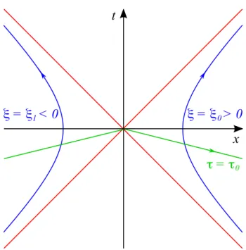
Coordinate curves are shaped as on fig. 3.2. Functions v~p,σ(τ, ~ξ) =θ(σλ) 1 p 2Ω(2π)s−1 e −iσΩ τ+ip·y_ψˆ ~ p(σζ) (3.12)

withσ =±1,λ≡λ(ξ) andζ= αξ_α+1, are solutions of Klein-Gordon equation and eigenfunctions ofλba_{. This solutions can be analytically extended to the}

whole Minkowski spacetime6 and constitutes a complete set [3]. Functions v~p,σ are called Rindler normal modes.

5_ξ∈(−1

α,∞) on region I andξ∈(−∞,− 1

α) on region II 6

Using the fact that surfaces with constantτ, which lie in I∪II, are Cauchy surfaces for the whole spacetime. This means that if you assign the value of solution of Klein-Gordon equation on these surfaces then you fixed its value on the whole spacetime.

x

t

�

=

�

> 0

�

=

�

< 0

��

=

�

Figure 3.2. Two curves with varyingτ and fixed opposite values ofξare marked

in blue; a curve with fixedτ is marked in green.

Expand the field with respect to solutionsv~p,σ:

φ(x) = Z ∞ 0 dΩ Z ds−1p X σ=±1 b~p,σv~p,σ(x) +b † ~ p,σv ∗ ~ p,σ(x)

Field quanta created by operators b†_p,σ~ are called Rindler particles. The vacuum is defined by

b~p,σ|0iR= 0 ∀~p, σ

3.2

Bogolubov transformations

The relation between the two particle definitions is expressed by Bogolubov coefficients (2.25). Consider α~_{k ~p,σ} = (u~_k, v~p,σ) = Z ¯ τ ds~ξ u~_k(x) _−i (αξ+ 1) ↔ ∂τ v_p,σ∗_~ (x)

It is convenient to use the surface ¯τ = 0, where t = 0, x = αξ_α+1 and ∂τ =λba∇a=λ(x∂t+t∂x) =λαξ_α+1∂t; substituting we have α_{~k ~}∗_p,σ = δ s−1_(k−p) 2√2πωΩ Z ∞ −∞ dζ θ(σλ) e −ik1ζ αζ (σΩ+λωζ) ˆψp~(σζ) (3.13) whereω≡ω~_k. Similarly β~_{k ~p,σ} = (v~p,σ, u~∗_k) = δs−1(k+p) 2√2πωΩ Z ∞ −∞ dζ θ(σλ) e ik1ζ αζ (σΩ−λωζ) ˆψp~(σζ) (3.14) The integrals in these expressions fundamentally are Fourier transformations of a Bessel function and are tabled. Note that

α~_{k ~p,σ} ∝δs−1(k−p) β~_{k ~p,σ} ∝δs−1(k+p)

so Bogolubov coefficients are distributions with respect to their indexes. Therefore expressions containing products of Bogolubov coefficients, as (2.26) and (2.27), are not well defined. From this it is possible to show that a uni-tary transformation that links the vacua of the two observers doesn’t exist7 [17]. This is only an apparent problem, indeed Bogolubov coefficients are distributions because in our case states with defined number are not nor-malizable (cf. (2.10)), for example

Mh0|a~ka

†

~

k|0iM =δ

s₍₀₎

This states belong to the Fock space F only in generalized sense. This situation is very common in Quantum Field Theory and is usually faced considering a field confined into a finite box and then taking the limit as the box side approaches infinity. In Rindler frame the solution of Klein-Gordon equation in a box is not simple, so we consider wave packets in the whole spacetime. Wave packets are normalizable states so they belong to the Fock spaceF in proper sense.

In order to obtain wave packets, consider the functionsf_~l(~k), with~l∈_Zs_,

such that Z f_~l(~_k)f∗ ~l0(~k) d s_~k=δ ~l~l0 and X ~l f_~l(~_{k) f}∗ ~l(~k0) =δs(~k−~k0)

These properties allow to derive from a set of functions{u_~k(x)}_~k∈

Rs that is

complete for F in generalized sense, a set {uˇ_~l(x)}_~l∈

Zs that is complete in

proper sense, through the relation ˇ u_~l(x)= Z f_~l(~_{k) u~} k(x) d s_~k (ˇu_~l,uˇ_~l0) =δ_~l~l0

You can found a possible set of functionsf_~l(~k) in [10]. The fieldφcan be expanded with respect to the ˇu_~l, giving

φ(x)= X ~l ˇ a_~luˇ_~l(x)+ ˇa† ~l uˇ ∗ ~l(x) ˇ a_~l = Z f_~l∗(~_{k) a~} k d s_{~k (3.15)}

Operators ˇa_~l satisfy the canonical commutation relations, moreover they define normalizable states, for example

h0|ˇa~_kˇa

†

~

k|0i= 1

Denote with ˇu_~l(x) wave packets obtained from plane waves (2.6) and

with ˇa_~l the relative annihilation operators. Denote with ˇvm~ (x)wave packets

obtained from Rindler modes (3.12) and with ˇbm~ the relative annihilation

operators. Bogolubov transformations between these two representation are regular and are linked to the previous by

ˇ α_{~l ~m} = (ˇu_~l,ˇvm~) = Z ds~k Z ds~p, σ f_~l(~_{k) f}∗ ~ m(~p,σ) α~_{k ~p,σ} ˇ β_{~l ~m} = (ˇvm~,uˇ_~l∗) = Z ds~k Z ds~p, σ f_~l(~_{k) fm~(~p,σ) β~} k ~p,σ (3.16) whereR ds~p, σ≡R∞ 0 dΩ R ds−1p P σ=±1.

Assuming that wave packets are always used, we can write “effective” versions of (3.13) and (3.14) [17], that are valid only if used through (3.16):

α_~∗ k ~p,σ ≡α eff∗ ~_{k ~p,σ} = 1 2π r Ω αω δ s−1_{(k−p) e}πΩ 2α Γ(iΩ α) ω+k1 ω−k1 iσ₂Ω_α β~_{k ~p,σ} ≡β~_{k ~}eff_p,σ = 1 2π r Ω αω δ s−1_{(k+p) e}−πΩ 2α Γ(iΩ_α) ω+k1 ω−k1 iσ₂Ω_α (3.17)

Substituting (3.16) and (3.17) into ˇbm~ = P ~l ˇ α_{~l ~m} ˇa_~l+ ˇβ_{~l ~}∗ m ˇa † ~l and us-ing (3.15) we find ˇ bm~ = Z ds~p, σ f_m∗_~(p,σ~ ) beff_~p,σ (3.18) where beff_~p,σ = Z ds~k α_~eff k ~p,σ a~k+β eff∗ ~ k ~p,σ a † ~_k

From (3.17) and the relation|Γ(ix)|2 ₌ π

xsinh(πx) we have beff_~p,σ = q N(Ω_α) + 1dΩ,p,σ+ q N(Ω_α) d†_{Ω,−p,−σ} (3.19) where N(Ω_α) = 1 e2πΩα −1 dΩ,p,σ = Z ∞ −∞ dk1 PΩ,p,σ(k1) ak1,p PΩ,p,σ(k1) = 1 √ 2πω1 ω1+k1 ω1−k1 −iσ₂Ω_α ω1 ≡ q k12+p2+m2

Operatorsd~p,σ are linear combinations of operators a~_k, so

d~p,σ|0iM = 0 ∀~p, σ

from which

beff_p,σ~ |0i_M =

q

N(Ω_α) d†_{Ω,−p,−σ}|0i_M (3.20) With a direct calculation you can show that operatorsd~p,σsatisfies canonical

commutation relations: [d~p,σ, d~p0_,σ0] = 0 [d† ~ p,σ, d † ~ p0_,σ0] = 0 [dp,σ~ , d†_~p0_,σ0] =δσσ0 δs(~p−p~0) (3.21)

Let us evaluate the mean value of the number operator of Rindler quanta on Minkowski vacuum with wave packets:

Mhˇ0|Nˇm~ |ˇ0iM =Mhˇ0|ˇb

†

~

mˇbm~ |ˇ0iM The state|ˇ0i_M is defined by

ˇ

that is satisfied by|0i_M (cf. (3.15)), so|ˇ0i_M =|0i_M.8 From (3.18) it follows that Mhˇ0|Nˇm~ |ˇ0iM = Z ds~p, σ Z ds~p0, σ0 fm~(~p,σ) fm~∗(~p0,σ0) Mh0|b eff ~ p,σ † beff_p~0_,σ0|0i M

From (3.20) and (3.21) we obtain

Mh0|b eff ~ p,σ † beff_~p0_,σ0|0i M = = q N(Ω_α)N(Ω_α0) _Mh0|dΩ,−p,−σd † Ω0_,−p0_,−σ0|0i_M = =N(Ω_α) δσσ0 δs(~p−~p0) In conclusion Mh0|Nˇm~ |0iM = Z ds~p, σ|f_m~(~p,σ)|2 1 e2πΩα −1

In particular, using functionsfm~ that are different from zero only on a small

region around a value~pm~, σm~, we have

Mh0|Nˇp~m~,σm~ |0iM ' 1 e

2π Ωm~

α −1

Mean value on Minkowski vacuum of the number operator of Rindler quanta with momentum ~pm~ is a Bose-Einstein distribution, at temperature

T = _2πkα

B, called Hawking-Unruh temperature. This temperature expressed

in MKS units is T = }α

2πkBc.

3.3

Thermalization theorem

The result just presented is the principal expression of the Unruh effect, and shows that Minkowski vacuum for an accelerated observer is equivalent to a thermal state. We can make more explicit the thermal nature of the relation between the two frames writing the Minkowski vacuum in terms of states with defined Rindler particle number.

Consider the inverse of (3.19) dΩ,p,σ= q N(Ω_α) + 1beff_Ω,p,σ− q N(Ω_α) beff_Ω,−†_p,−σ 8_{Similarly|ˇ0i} R=|0iR.

Substituting into d~p,σ|0iM = 0 we have beff_Ω,p,σ−e−πΩα beff† Ω,−p,−σ |0i_M = 0 (3.22)

Considering wave packets it becomes

ˇ bΩm~,pm~,σm~ −e −πΩ ~m α ˇb† Ωm~,−pm~,−σm~ |0i_M = 0

To simplify notation consider a single normal mode, on regions I and II with oppositepm~, so ˇ_bσ−e−A_ˇb† −σ |0i_M = 0 (3.23) withA=πΩm~

α . Expand the state |0iM with respect to Rindler states

|0i_M = X n+,n− cn+,n− |n+, n−iR |n+, n−iR = (ˇb†₊)n+ _(ˇb† −)n− p n+!n−! |0i_R

Substituting into (3.23) we get

         X n+,n− _p n++ 1cn++1,n−−e −A√_n − cn+,n−−1 |n₊, n−iR = 0 X n+,n− _p n−+ 1cn+,n−+1−e −A√_n + cn+−1,n− |n₊, n−iR = 0

from which we have the recursive relations

( p n++ 1cn++1,n− =e −A√_n − cn+,n−−1 p n−+ 1cn+,n−+1 =e −A√_n + cn+−1,n−

This system is satisfied by cn+,n− =

√

B e−n+A _δ

n+,n− (3.24)

whereB is a constant; substituting

|0i_M =√B X n e−nA (ˇb†₊)n (ˇb†−)n n! |0iR= √ B expe−Aˇb₊† ˇb†₋ |0i_R (3.25)

The constant B is determined by the normalization: Mh0|0iM =B X n e−2nA=B e 2A e2A₋₁ = 1 SoB = (1−e−2A_{) and} |0i_M =p1−e−2A _expe−A_ˇb† +ˇb † − |0i_R

Considering all normal modes we have the correct expression:

|0i_M = Y ~ m q 1−e− 2_{πΩ ~m} α ! exp X ~ m e−πΩ ~αm ˇb† Ωm~,pm~,σm~ ˇ_b† Ωm~,−pm~,−σm~ ! |0i_R

Minkowski vacuum can be written as a Rindler state for which there is entanglement9 between regions I and II: if you find nm~ particles with

mo-mentumΩm~,pm~ in region I, then you will findnm~ particles with momentum

Ωm~,−pm~ in region II.

Note that accelerated observers in region I and that in region II can’t communicate10, so there isn’t any causal relation among them (see fig. 3.3).

Measures carried out by accelerated observers in regi