Semiparametric Conditional Quantile Estimation through
Copula-Based Multivariate Models
HohsukNoh
Universit´e catholique de Louvain
Anouar El Ghouch Universit´e catholique de Louvain Ingrid Van Keilegom
Universit´e catholique de Louvain April 18, 2014
Abstract
We consider a new approach in quantile regression modeling based on the copula function that defines the dependence structure between the variables of interest. The key idea of this approach is to rewrite the characterization of a regression quantile in terms of a copula and marginal distributions. After the copula and the marginal distributions are estimated, the new estimator is obtained as the weighted quantile of the response variable in the model. The proposed conditional estimator has three main advantages: it applies to bothiidand time series data, it is automatically monotonic across quantiles, and, unlike other copula-based methods, it can be directly applied to the multiple covariates case without introducing any extra complications. We show the asymptotic properties of our estimator when the copula is estimated by maximizing the pseudo log-likelihood and the margins are estimated nonparametrically including the case where the copula family is misspecified. We also present the finite sample performance of the estimator and illustrate the usefulness of our proposal by an application to the historical volatilities of Google and Yahoo companies.
Key words: Dependence Modeling; Check function; Markov Process; Pseudo Log-likelihood; Vine copula.
1
Introduction
Appropriate understanding and modeling of the dependence structure between financial assets is an important task. Especially, the characterization of the conditional dependence between random variables at a give quantile constitutes an important ingredient in modern risk management. As a copula has emerged as an effective tool to model dependence between non-elliptic and fat-tailed random variables, several authors attempted to propose conditional quantile estimation methods which are able to make use of the advantages of copulas in dependence modeling. Their common starting point is that since the copula function holds all information on the different forms of dependence between random variables, the form of the conditional quantile relationship is implied by the copula joining those random variables.
Some examples of such work include Bouy´e and Salmon (2009), Chen and Fan (2006) and Chen et al. (2009). In an earlier version of Bouy´e and Salmon (2009), the authors explicitly showed the link between the form of the conditional quantile relationship and the copula function for several well-known copula families such as elliptical copulas and Archimedean copulas. Further, they illustrated how such link can be used in conditional quantile estimation both when modeling the interdependence between random variables and when modeling the temporal dependence between them. Focusing more on the latter case, Chen and Fan (2006) studied a class of univariate copula-based stationary Markov models. Under the assumption of correct specification of the parametric copula, Chen and Fan (2006) established asymptotic properties of their quantile regression estimator when the copula is estimated by maximizing the pseudo log-likelihood and the marginals are estimated nonparametrically. Additionally, also in the time series context, Chen et al. (2009) employed parametric copula models to propose several distinct nonlinear quantile autoregression models and investigated the asymptotic properties of their estimator when both the copulas and the marginals could be globally misspecified but assuming the correct specification of a conditional quantile function at a particular quantile.
However, all these works consider a conditional quantile given just one covariate such as the conditional quantile ofY given X or the conditional quantile of Yt given its lagged observation Yt−1.
Nevertheless, often it is necessary to consider multivariate quantile regression conditioning on more than one covariate. Apart from examples in the iid setup, there are many such examples in the time series setting where the copula-based quantile estimation methods should be extended. One example is a copula-based Markov process of higher order, for which Ibragimov (2009) studied how a copula characterizes the statistical properties of the corresponding Markov process. However, they
did not investigate the issue of the conditional quantile estimation there. Another example is copula-based multivariate time series models, where for instance the dependence between two Markovian (stationary) time seriesXtandYtis modeled via a copula which characterizes the dependence between Xt−1, Yt−1, XtandYt, in other words, serial dependence and interdependence between two time series.
R´emillard et al. (2012) discussed parameter estimation and goodness-of-fit testing for this model but did not address the issue of quantile estimation such as the conditional quantile ofYtgivenXt−1, Yt−1
and Xt.
Based on this observation, we are motivated to develop an extended version of the previous copula-based quantile regression methods to handle multiple covariates. The key idea of the previous methods is to express the conditional distribution function in terms of a certain partial derivative of the copula function and the marginal distributions, and obtain the conditional quantile through it. Although it is possible to consider an extension based on this idea, we find it better for convenient computation and concise theoretical development to estimate the conditional quantile function directly using the so-called ‘check’ function in Koenker and Bassett (1978) without going through the conditional distri-bution. The main idea of our new approach is to rewrite the check-function based characterization of a regression quantile in terms of a copula function and marginal distributions. Actually, our proposal is an extension of the recent work of Noh et al. (2013) from mean regression to quantile regression. However, non-differentiability of the check loss function in quantile regression makes the extension nontrivial, which needs a separate treatment. Additionally, to broaden the area of application, we derive the asymptotic properties of the estimator under general conditions where both the iid setting and the time series setting can be considered.
The rest of this paper is organized as follows. In Section 2, we introduce our conditional quantile estimation method. We present the asymptotic properties of the proposed estimator in Section 3 and present the finite sample performance of our estimator via some numerical simulations both in the
iid and time series setting in Section 4. Finally, we analyze the daily log returns data of Google and Yahoo companies in Section 5 to illustrate the usefulness of our proposal. All technical details are deferred to the Appendix.
2
Copula-based Quantile Regression Estimator
Let X = (X1, . . . , Xd) be a covariate vector of dimension d ≥1 and Y be a response variable with continuous cumulative distribution functions (c.d.f.s) F1, . . . , Fd and F0, respectively. We denote
the density ofXj and Y by fj and f0, respectively. For a given x= (x1, . . . , xd)⊤, from the seminal work of Sklar (1959), the c.d.f. of (Y,X) evaluated at (y,x) can be expressed asC(F0(y),F(x)).Here,
F(x) = (F1(x1), . . . , Fd(xd))⊤andCis the copula distribution of (Y,X) defined byC(u0, u1, . . . , ud) = P(U0 ≤u0, U1 ≤u1, . . . , Ud ≤ud), where U0 =F0(Y) and Uj =Fj(Xj), j = 1, . . . , d. The copula C
is considered to hold all information on the dependence of (Y,X) since it joins the marginals together to give the joint distribution. Naturally, it is expected that a given copula function implies a certain form of the conditional quantile relationship.
More precisely, the following link holds between the copula and the conditional distribution when the dimension ofX is one:
∂C(u0, u1)
∂u1
=FY|X1(F−
1
0 (u0)|F1−1(u1)),
where FY|X1 is the conditional distribution of Y given X1. From this link, the conditional quantile
functionmτ(x1) of Y given X1 =x1 is derived in terms of the copula function and the marginals:
mτ(x1) =F0−1(QU0|U1(τ|F1(x1))), (1) where QU0|U1(τ|u1) is the conditional τ-quantile function of U0 given U1 = u1, which is the inverse function of ∂C(u0, u1)/∂u1 with respect to u0. The expression (1) is the key idea underlying the
previous works (Chen and Fan, 2006; Bouy´e and Salmon, 2009; Chen et al., 2009). Although it is possible to consider the extension of the relation (1) to multiple covariate case (d≥2), we use another link between the conditional quantile and the copula via the check function to propose an extension which has computational convenience and for which concise asymptotic theory can be easily developed. For that purpose, we note that from the definition of copula function, the conditional density of Y givenX =xis expressed as
f0(y)c(F0(y),
F(x))
cX(F(x)) , (2)
where c(u0,u)≡c(u0, u1, . . . , ud) =∂d+1C(u0, u1, . . . , ud)/∂u0∂u1. . . ∂udis the copula density corre-sponding to C and cX(u) ≡cX(u1, . . . , ud) = ∂dC(1, u1, . . . , ud)/∂u1. . . ∂ud is the copula density of X. Interestingly, thanks to the expression (2), the τ-conditional quantile mτ(x) of Y given X =x
can be written in terms of the copula and the marginals as follows: mτ(x) = arg min a E[ρ(Y −a)|X =x] = arg min a E[ρ(Y −a) c(F0(Y),F(x))], (3) whereρ(y)≡ρτ(y) =y(τ−I(y <0)) is the well known check function. Note that different from (1), the expression (3) is not affected by the dimension of the covariate vector X.
If ˆc, ˆF0 and ˆFj are any given estimators forc,F0 and Fj,j= 1, . . . , d, respectively, thenmτ(·) can be estimated by ˆ mτ(x) = arg min a n X i=1 ρ(Yi−a) ˆc( ˆF0(Yi),Fˆ(x)), (4)
where ˆF(x) = ( ˆF1(x1), . . . ,Fˆd(xd))⊤. Note that the estimator in (4) has the monotonicity across
quantile levels. It can be shown using the argument in the proof of Theorem 2.5 of Koenker (2005). Following the argument there, one can prove that
(τ2−τ1)( ˆmτ2(x)−mˆτ1(x)) n X i=1 ˆ c( ˆF0(Yi),Fˆ(x))≥0.
Since ˆc≥0, this implies that ˆmτ2(x)≥mˆτ1(x) whenever τ2 ≥τ1.
Since there are many different methods available in the literature for estimating a copula and a c.d.f., ˆm(x) can be a nonparametric or a semiparametric or a fully parametric estimator depending on the method of estimating the components in (4). In this paper, we consider a semiparametric approach where the copula is parametrized but the marginal distributions are left unspecified as in Noh et al. (2013). Specifically, we assume a certain parametric family of copula densities, C = {c(u0,u;θ), θ∈Θ}, where Θ is a compact subset of Rp, to which the true copula density belongs or
by which it is well approximated.
3
Asymptotic Properties of the Proposed Estimator
In this section, we first provide general assumptions about the estimator, which will allow us to investigate its asymptotic properties both in the iid and dependent settings. Then, we will present the asymptotic representation of the estimator derived from the assumptions.
3.1 Assumptions
Before stating the assumptions, we introduce some notations, which will be used throughout the asymptotic analysis of our estimator. As mentioned in the previous section, we consider a certain family of copula densities, C = {c(u0,u;θ), θ ∈Θ}, for estimating the true density c(u0,u). Define
θ∗ to be the (unique) pseudo-true copula parameter which lies in the interior of Θ and minimizes I(θ) = Z [0,1]d+1 ln c(u0,u) c(u0,u;θ) dC(u0,u).
Here,I(θ) is the classical Kullback-Leibler information criterion expressed in terms of copula densities instead of the traditional densities. It is clear that when the true copula density belongs to the given family, i.e. c(.) = c(.;θ0) for a certain θ0, then we have θ∗ = θ0. Additionally, we let cX(u;θ) =
R
c(u0,u;θ)du0. Also define
fθ(y|x) =f0(y)c(F0(y),
F(x);θ)
cX(F(x);θ) and mτ(x;θ) = arg miny
E[ρτ(Y −y)c(F0(Y),F(x);θ)]. Concerning the partial derivatives of the copula density, we define
Djc= ∂c ∂uj , j = 0, . . . , d, c′ = (D1c, . . . , Ddc)⊤ and ˙c= ∂c ∂θ1 , . . . , ∂c ∂θp ⊤ .
Here are the assumptions for our estimator.
(C0) {Yi}i≥1 is a strictly stationary process with β-mixing coefficient β(i) satisfying β(i) =O(i−ν),
asi→ ∞, for some ν >1.
(C1) ˆF(x)−F(x) = Op(n−1/2), where ˆF(x) = ( ˆF1(x1), . . . ,Fˆd(xd))⊤ and ˆFj(·) is an estimator for Fj(·).
(C2) ˆθ−θ∗ =Op(n−1/2), where ˆθ is an estimator ofθ∗.
(C3) Let g denote either c˙ or Djc, j = 0, . . . , d and x ∈ Rd be a given point of interest such that F(x)∈(0,1)d.
(i) c(1,F(x);θ∗)<∞,c(0,F(x);θ∗)<∞ and 0< cX(F(x);θ∗)<∞;
(ii) (u,θ)7→g(u0,u;θ) is continuous in (u,θ) at (F(x),θ∗) uniformly in u0 ∈[0,1];
(C4) f0 is continuous atmτ(x;θ∗).
(C5) y7→fθ∗(y|x) is continuous atmτ(x;θ∗) andfθ∗(mτ(x;θ∗)|x)>0.
Assumption (C3) is satisfied for many popular copula families. (C4) and (C5) are typically assumed in quantile regression. Hence, in the following we will give some examples where (C0), (C1) and (C2) are satisfied in the iidsetting and the time series setting.
3.1.1 IID setting
Suppose that we have (Yi,Xi), i = 1, . . . , n, an independent and identically distributed (iid) sample of n observations generated from the distribution of (Y,X). In this case, (C0) is trivially satisfied. Concerning (C1), it is satisfied with the empirical distribution ofXj and its rescaled version which is popular in copula estimation context and is defined by
ˆ Fjs(xj) = 1 n+ 1 n X i=1 I(Xj,i≤xj).
Additionally, we can also use kernel smoothing method for estimating Fj(·), j = 1, . . . , d. Let k(·) be a function which is a symmetric probability density function and h ≡ hn → 0 be a bandwidth parameter. Then, a kernel smoothing estimator ˜Fj is given by
˜ Fj(xj) = 1 n n X i=1 K xj−Xj,i h ,
where K(x) = R−∞x k(t)dt. If nh4 → 0 holds for the bandwidth h, then for ˆFj = ˜Fj, the following condition is satisfied:
(C1’) ˆFj(xj) =n−1Pni=1I(Xj,i≤xj) +op(n−1/2),
from which (C1) follows. One advantage of using ˜Fj is that it results in a smooth estimate ˆmτ(x), whereas the empirical distribution or its rescaled version does not. As for (C2), one example of the estimator ˆθthat satisfies (C2) in the literature is the maximum pseudo-likelihood (PL) estimator ˆθP L, which maximizes L(θ) = n X i=1 logcFˆ0s(Yi),Fˆs(Xi);θ , (5)
where ˆFs(Xi) = ( ˆF1s(X1,i), . . . ,Fˆds(Xd,i))⊤. The estimator ˆθP L was studied by several authors in-cluding Genest et al. (1995), Klaassen and Wellner (1997), Silvapulle et al. (2004), Tsukahara (2005)
and Kojadinovic and Yan (2011), etc. If the score function of c(u0,u;θ) satisfies the assumptions
(A.1)-(A.5) given in Tsukahara (2005), the PL estimator satisfies (C2) even when the copula family is misspecified as checked in Noh et al. (2013).
3.1.2 Time series setting
Assumptions under which a copula-based Markov process satisfies α-mixing or β-mixing have been studied by many authors. For example, if {Yi}i≥1 is a (stationary) univariate first-order Markov
process and the copula of (Yi, Yi−1) ≡ (Yi, Xi,1) satisfies certain conditions (see Proposition 2.1 of
Chen and Fan (2006)), then Assumption (C0) holds and hence (C1) also holds with any estimator ˆ
Fj(·) satisfying (C1’) (see Rio (2000)). Following similar ideas, R´emillard et al. (2012) extended this result to the case of copula-based multivariate first-order Markov process. As for copula-based Markov processes of higher order, unfortunately such results are rare. The only related work that we have found is Ibragimov (2009), who obtained a characterization of higher-order Markov processes in terms of copulas, but he did not discuss the mixing properties of the resulting process.
Concerning Assumption (C2), if we consider an extension of the maximum pseudo likelihood estimator studied by Genest et al. (1995) to the Markovian case, the resulting estimator satisfies (C2). For example, suppose that we have a sample {(Yi, Xi) : i = 1, . . . , n} of a multivariate first-order Markov process generated from (F0(·), F1(·), c(·,·,·,·;θ∗)), where c(·,·,·,·;θ∗) is the true parametric
copula density associated with (Zi,Zi−1) with Zi = (Yi, Xi)⊤ up to the unknown value θ∗. If we consider the following estimator for θ∗,
ˆ
θP Ldep= arg max θ∈Θ n X i=2 log ( c( ˆUi,Uˆi−1;θ) q( ˆUi−1;θ) ) , (6) where ˆ F0s(·) = 1 n+ 1 n X i=1 I(Yi ≤ ·), Fˆ1s(·) = 1 n+ 1 n X i=1 I(Xi≤ ·), Uˆi= ( ˆF0s(Yi),Fˆ1s(Xi))⊤, q(u2, u3;θ) = Z 1 0 Z 1 0 c(u0, u1, u2, u3;θ)du1du0,
then (C2) holds according to Theorem 1 in R´emillard et al. (2012) under the assumptions (A1)-(A4) that they provided. For univariate copula-based first-order Markov models, a similar result can be found in Chen and Fan (2006).
3.2 Asymptotic representation of the estimator mˆτ(x)
To realize the theoretical analysis of our estimator, we begin by introducing a few more notations: • Fˆ0(y) =n−1Pni=1I(Yi ≤y).
• ǫi≡ǫi(x;θ∗) =Yi−mτ(x;θ∗).
• e′(x) =Eψτ(ǫi)c′(F0(Y),F(x);θ∗) and ˙e(x) =E[ψτ(ǫi) ˙c(F0(Y),F(x);θ∗)], whereψτ(y) =τ−I(y≤0).
Now we are ready to present the asymptotic representation of the proposed estimator.
Theorem 3.1 Suppose that Assumptions (C0)-(C5) hold. Then, we have
√ n( ˆmτ(x)−mτ(x;θ∗)) = 1 f0(mτ(x;θ∗))c(F0(mτ(x;θ∗)),F(x);θ∗) Un+op(1), where Un = √n( ˆF(x)−F(x))⊤e′(x) +√n( ˆθ−θ∗)⊤e˙(x) −√nFˆ0(mτ(x;θ∗))−F0(mτ(x;θ∗)) c(F0(mτ(x;θ∗)),F(x);θ∗).
Theorem 3.1 implies that the estimator ˆmτ(x) converges in probability tomτ(x;θ∗) asn→ ∞. Hence, when the copula family is misspecified, the estimator ˆmτ(x) is no more consistent. In such situation, since c(·;θ∗) is just the best approximation to the true copula density c(·), we have a bias in the estimation of the true conditional quantile function ˆmτ(x), which is (asymptotically) the difference betweenmτ(x) and its best approximation mτ(x;θ∗) among the function class{m(x;θ) :θ ∈Θ}.
As an application of Theorem 3.1, we consider the asymptotic normality of the estimator, for which we have to make a stronger assumption than (C2):
(C2’) ˆθ−θ∗ =n−1Pni=1ηi+op(n−1/2), whereηi =η(U0,i,Ui;θ∗) is a p-dimensional random vector such thatEη=0 and Eη⊤η<∞ and Ui= (U1,i, . . . , Ud,i)⊤.
This stronger assumption also holds for ˆθP L in theiid setting and ˆθdepP L in the time series setting with the same conditions for (C2). For the iidcase, the function η is given by
where J(θ) = Z [0,1]d+1 − ∂ 2 ∂θ∂θ⊤ logc(u0,u;θ) dC(u0,u)
and K(U0,U;θ) is a p-dimensional vector whose k-th element is
∂ ∂θk logc(U0,U;θ) + d X j=0 Z [0,1]d+1 (I(Uj ≤uj)−uj) ∂2 ∂θk∂uj logc(u0,u;θ) dC(u0,u).
Concerning the time series case, see Chen and Fan (2006) for the univariate case and R´emillard et al. (2012) for the multivariate case. Replacing (C2) with (C2’) in the previous assumptions, we have an asymptotic linear representation of the conditional quantile estimator ˆmτ(x), which implies the asymptotic normality of ˆmτ(x).
Corollary 3.2 Suppose that Assumptions (C0)-(C1), (C1’), (C2’), (C3)-(C5) hold. Then, we have
√ n( ˆmτ(x)−mτ(x;θ∗)) = √1 n n X i=1 hXd j=1
{I(Xj,i≤xj)−Fj(xj)}ej(x) +η⊤i e˙(x)− {I(Yi ≤mτ(x;θ∗))−F0(mτ(x;θ∗))} ×c(F0(mτ(x;θ∗)),F(x);θ∗)
i
[f0(mτ(x;θ∗))c(F0(mτ(x;θ∗)),F(x);θ∗)]−1+op(1) (8)
where e′(x) = (e1(x), . . . , ed(x))⊤.
Specifically, Corollary 3.2 implies that √n( ˆmτ(x)−mτ(x;θ∗)) follows asymptotically a normal distribution with mean 0 and variance σ2=Var(E1) + 2P∞
j=1Cov(Ej+1, E1), whereEi denotes each summand in the summation of (8) (see Theorem 4.2 in Rio (2000)). Especially, since σ2 =Var(E
1)
when the data areiid, we can estimateσ2by an estimator ˆσ2 =n−1Pni=1ncEi−n−1Pni=1cEi
o2
, where
c
Ei is an estimator ofEiobtained by replacing all the unknown quantities inEi by their corresponding estimates, for example,θ∗ by ˆθ andF0 by ˆF0. Thanks to this estimator ˆσ, we can easily calculate the
confidence interval formτ(x;θ∗) using Corollary 3.2.
However, according to our simulation studies (see Section 4), the accuracy of the coverage of this confidence interval seems to sensitively depend on the accuracy of the estimation of the unknown quantities involved in Ei. Due to this, we propose to use a bootstrap method to approximate the asymptotic variance of the estimator ˆmτ(x). The bootstrap that we use for the iid data in our simulations is outlined below:
Step 0: Obtain the copula parameter estimate ˆθfrom (5) and the marginal distribution estimates ˜
F0 and ˜Fj using the kernel smoothing method with appropriate bandwidths h0,n and hj,n, j= 1, . . . , d.
Step 1: Generate n independent random vectors Ui = (U0b,i, . . . , Ud,ib )⊤, i = 1, . . . , n from the estimated copulac(u0, . . . , ud; ˆθ), where Ui = (U0,i, . . . , Ud,i)⊤.
Step 2: Let Yib= ˜F0−1(U0,i) and Xj,ib = ˜Fj−1(Uj,i), j = 1, . . . , d.
Step 3: Repeating Steps 1 and 2 a large number of times, compute the bootstrap values ˆ
mbτ(x), b = 1, . . . , B of the estimator ˆmτ(x) and then calculate the estimate of the asymp-totic variance using them:
ˆ σ2boot = 1 B B X b=1 ( ˆmbτ(x))2− 1 B B X b=1 ˆ mbτ(x) !2 .
Following similar ideas but modifying Steps 0 and 1 (see Section 4.3 in Chen and Fan (2006) and Section 2 in R´emillard et al. (2012)), we can estimate the asymptotic variance σ2 in the time
series setting using a bootstrap procedure. In Section 4, we investigate how the proposed bootstrap procedures perform by checking the coverage probabilities of the confidence interval for ˆmτ(x) based on this procedure. In our simulations, we observe that it is important for satisfactory accuracy of the coverage of the confidence interval to use the kernel smoothing estimates of the marginal distributions following the concept of the smoothed bootstrap (Silverman and Young, 1987) in both the iid and time series setting. If we use the empirical distribution or its rescaled version, the coverage probability of the confidence interval does not approach the nominal confidence level at all.
4
Numerical Results
In this section, we firstly check whether the asymptotic theory for ˆmτ(x) works both in the iid setting and in the time series setting. Secondly, we compare our semiparametric estimator with some competitors. For this purpose, we consider the following data generating processes (DGP):
– The resulting quantile regression function is
mτ(x1) =F0−1((1 +F1(x1)−α(τ−α/(1+α)−1))−1/α).
• DGP B(F0(Y), F1(X1), . . . , Fd(Xd))∼Gaussian copula with correlation matrix Σ =
1 ρ ⊤ ρ ΣX
– The resulting quantile regression function is
mτ(x) =F0−1 Φ d X j=1 ajΦ−1(Fj(xj)) +p1−ρ⊤aΦ−1(τ)
wherea= (a1, . . . , ad)⊤= Σ−X1ρ and Φ(·) is the c.d.f. of a standard normal distribution. Although we describe each DGP with the focus on the iid setting, it can be also described for the time series setting. For example, using DGP A with Y =Yi, X1 = Yi−1 and F0 = F1 = F, we can
generate a sample{Yi}ni=1from a univariate first-order Markov model. Then, the conditional quantile function of Yi given Yi−1 =y is given by mτ(y) = F−1((1 +F(y)−α(τ−α/(1+α)−1))−1/α). Table 1
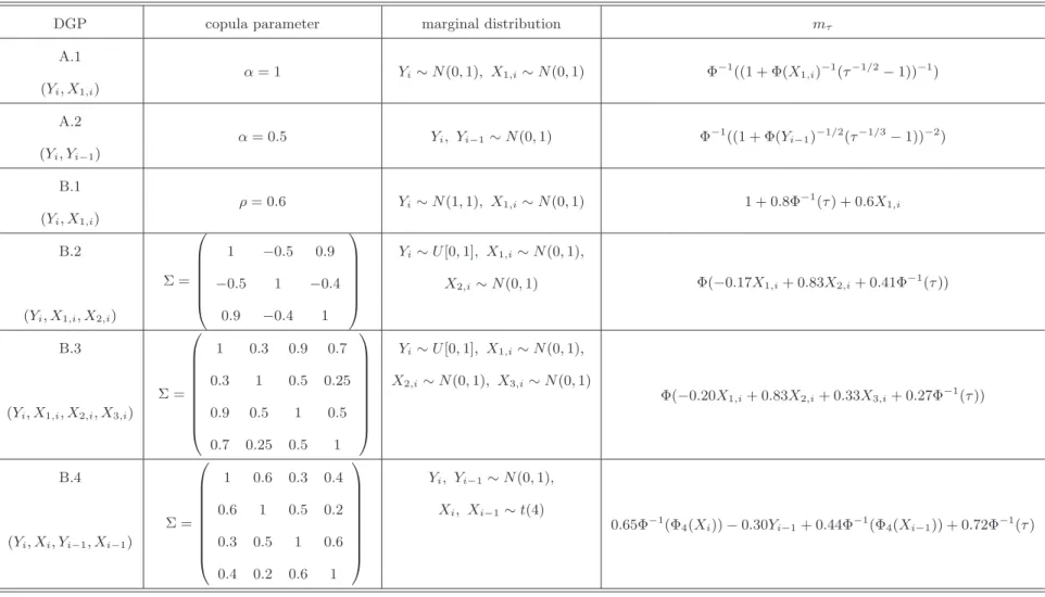
shows the parameters of the copula and the marginal distributions of each DGP subspecialized from DGPs A and B. All computations are done with R (R Development Core Team, 2011)
4.1 Verifying the asymptotic results about mˆτ(x)
In this section, to verify the established asymptotic results, we compute a confidence interval formτ(x) either by the asymptotic representation or the bootstrap proposed in Section 3. By verifying whether the empirical coverage probabilities (ECP) of the (1−α)-confidence interval formτ(x) are close to the nominal confidence level (1−α), we indirectly check whether the estimator ˆmτ(x) is asymptotically normal.
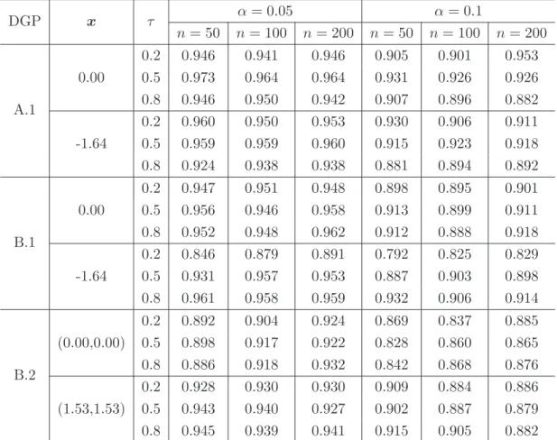
First, concerning theiid setting, we generate 500 random samples of sizen= 50,100 and n= 200 from DGPs A.1, B.1 and B.2 and compute a confidence interval for mτ(x) using ˆσ2 and Corollary 3.2. Table 2 shows the ECP of the (1−α)-confidence interval for mτ(x) withα = 0.05 and 0.1. We observe that depending on the location of the covariates and the quantile level, sometimes the ECP has a quite different value from its nominal confidence level. As mentioned before, the main reason for this is the inaccuracy of the estimation of the unknown quantities involved in the asymptotic
Table 1: The copula parameters and the marginal distributions for each subspecialized DGP. Φν(·) is the c.d.f. of a random variable t(ν).
DGP copula parameter marginal distribution mτ
A.1 α= 1 Yi∼N(0,1), X1,i∼N(0,1) Φ−1((1 + Φ(X1,i)−1(τ−1/2−1))−1) (Yi, X1,i) A.2 α= 0.5 Yi, Yi−1∼N(0,1) Φ−1((1 + Φ(Yi−1)−1/2(τ−1/3−1))−2) (Yi, Yi−1) B.1 ρ= 0.6 Yi∼N(1,1), X1,i∼N(0,1) 1 + 0.8Φ−1(τ) + 0.6X1,i (Yi, X1,i) B.2 Σ = 1 −0.5 0.9 −0.5 1 −0.4 0.9 −0.4 1 Yi∼U[0,1], X1,i∼N(0,1), Φ(−0.17X1,i+ 0.83X2,i+ 0.41Φ−1(τ)) X2,i∼N(0,1) (Yi, X1,i, X2,i) B.3 Σ = 1 0.3 0.9 0.7 0.3 1 0.5 0.25 0.9 0.5 1 0.5 0.7 0.25 0.5 1 Yi∼U[0,1], X1,i∼N(0,1), Φ(−0.20X1,i+ 0.83X2,i+ 0.33X3,i+ 0.27Φ−1(τ)) X2,i∼N(0,1), X3,i∼N(0,1) (Yi, X1,i, X2,i, X3,i) B.4 Σ = 1 0.6 0.3 0.4 0.6 1 0.5 0.2 0.3 0.5 1 0.6 0.4 0.2 0.6 1 Yi, Yi−1∼N(0,1), 0.65Φ−1 (Φ4(Xi))−0.30Yi−1+ 0.44Φ− 1 (Φ4(Xi−1)) + 0.72Φ− 1 (τ) Xi, Xi−1∼t(4) (Yi, Xi, Yi−1, Xi−1)
representation. As is typical in quantile regression, the asymptotic representation for ˆmτ(x) involves the conditional density fY|X(mτ(x)|x), which is equal to f0(mτ(x;θ∗))c(F0(mτ(x;θ∗)),F(x);θ∗)
when the copula family is correct. Since it controls the scale of the estimated asymptotic variance of ˆ
mτ(x), the estimation accuracy of it seems to affect the ECP a lot. To confirm our claim, we evaluate the asymptotic representation using the true values of all involved quantities and compute the ECP. As was expected, we observe in Table 3 that the recalculated ECP is close to the nominal confidence level as the sample size increases. Finally, we compute the confidence interval and its ECP using the bootstrap (B = 200) proposed in Section 3. Table 3 suggests that the bootstrap method seems to solve the problem more or less.
To verify the asymptotic behavior of our estimator under misspecification, we generate data from a Clayton copula according to DGP A.1 but in the estimation procedure we use a Gaussian copula. The ‘pseudo’-true quantile regression function ismτ(x1;ρ∗) = Φ−1(τ)
p
1−ρ∗2+ρ∗x1 withρ∗ = 0.503 for
the Clayton copula withα = 1. Figure 1 shows the boxplots of the estimators ˆmτ(x1) obtained from
500 random samples of size 200. We see that the observed values are symmetrically distributed around the pseudo-true parametermτ(x1;ρ∗) instead of the true parametermτ(x1) as expected according to
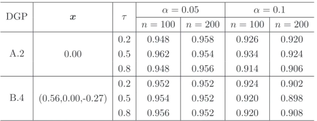
Theorem 3.1. The difference between these two quantities corresponds exactly to the asymptotic bias. As for the time series setting, we generate 500 random samples of size n = 100 and 200 from DGPs A.2 and B.4. To compute a confidence interval for mτ(x), we estimateσ2 using the bootstrap described in Section 3 with B = 200. We observe that the bootstrap seems to work reasonably well in terms of the ECP as shown in Table 4. The ECP when α= 0.1 seems to be somewhat higher than the nominal confidence level but gets closer to it as the sample size grows.
4.2 Comparison with other methods
In this subsection we compare our semiparametric estimator both with semiparametric and nonpara-metric competitors. We consider four estimators for comparison.
• mtcˆ : our estimator when the true copula family is used.
• mucˆ : our estimator when the copula density family is adaptively selected using the data (see the explanation below).
• mˆll : local linear estimator with the bandwidth selected by cross-validation based on the check-function.
• mˆsi : single index regression estimator based on a two stage estimation method; the single-index coefficients are first estimated by the method of Zhu et al. (2012), and then the link function is estimated in the same way as for ˆmll.
In addition to this, we consider the nonlinear quantile regression estimator ˆmnl, which exploits the true link function as a reference case. We use the R packagequantregto calculate ˆmnl. Concerning the estimator ˆmuc, we use the simplified pair-copula decomposition of the copula density (R-vine) as in Noh et al. (2013). The main idea of it is to decompose a multivariate copula to a cascade of bivariate copulas so that we can take advantage of the relative simplicity of bivariate copula selection and estimation. For details, we refer to Aas et al. (2009), Brechmann (2010), Noh et al. (2013) and references therein. Specifically, we choose one decomposition of the copula density (among many R-vine structures) for the data, and then choose the pair-copulas independently among ten candidate copulas: two are elliptical (Gaussian and Studentt) and eight are Archimedean (Clayton, Gumbel, Frank, Joe, Clayton-Gumbel, Joe-Gumbel, Joe-Clayton and Joe-Frank) using the R package VineCopula. As a selection criterion for bivariate copulas, we use the Akaike information criterion (AIC), which is shown to work in this context (see Dißmann et al. (2013)).
For comparison with other methods, we consider DGPs B.2 and B.3 to generate data. For perfor-mance evaluation of each method, we consider the empirical integrated mean squared error (IMSE), which is defined by IMSE = 1 N N X l=1 ISE( ˆm(τl)) = 1 N N X l=1 " 1 I I X i=1 ˆ m(τl)(xi)−mτ(xi)2 # ,
where{xi,i= 1, . . . , I}is a fixed evaluation set which corresponds to a random sample of sizeI = 500 generated from the distribution of X, ˆm(l)(·) is the estimated regression function from the l-th data sample. As expected, the estimator ˆmnl performs best in both DGPs. Our estimator ˆmtc, which uses the information about the copula family, ranks the second. Additionally, even the estimator ˆmuc is a bit behind ˆmtc in performance due to the pair-copula selection step before the estimation, but it is still advantageous over the other semiparametric estimator ˆmsiand the nonparametric estimator ˆmnp. From this observation, we see that when the true DGP can be described using a certain copula which belongs to the copula family under consideration, which is the case here, our proposed methods can be a good choice in quantile regression. However, the performance of our estimators may depend on whether the true copula density fits into the copula family under our consideration or not. To see the
impact of it, we consider an additional DGP.
• DGP CY =m(X1, X2, X3) +σǫ, where ǫ∼N(0,1) independent ofX.
– m(X1, X2, X3) = Ψ(−0.3X1+ 0.9X2+ 0.3X3) where Ψ is the c.d.f. of the standard Cauchy
distribution andσ= 0.1
– The resulting quantile regression function is Ψ(−0.3X1+ 0.9X2+ 0.3X3) + 0.1Φ−1(τ).
– X = (X1, X2, X3)⊤ is multivariate normal with mean 0and cov(Xj1, Xj2) = 0.5| j1−j2|.
Table 7 shows the performance of each method. Note that since we have no knowledge about the true copula, the estimator ˆmtcis not available. In this case, as before the estimator ˆmnl performs best but the single-index estimator ranks the second in most cases. However, our estimator ˆmucstill shows comparable performance to ˆmsi and performs better than the nonparametric estimator ˆmnp. This suggests that the copula family under consideration is flexible enough to approximate the true copula density in a certain degree although it does not include the density. Additionally, it also implies that our method has the advantage over the classical single-index model and that it is more flexible and adapts better to different settings.
5
Empirical Application
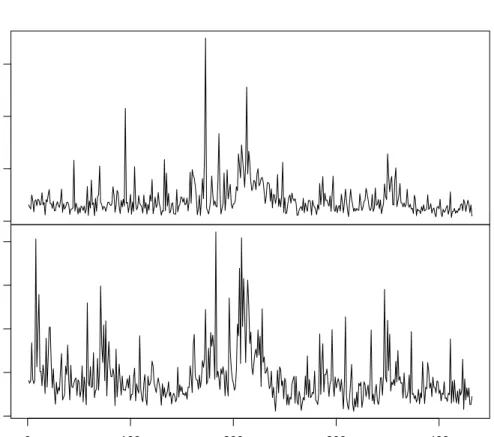
To illustrate the usefulness of our method, we analyze the historical volatilities of Yahoo({Yi}) and Google({Xi}) companies over a nine-year period (2004-2013, 2160 trading days). Every 5 trading days we compute the standard deviation of the log returns of each company and consider it as the historical volatility of the period. The volatilities of both companies over the whole period are plotted in Figure 2 (432 observations for each time series). When the volatility data for both companies in a certain length of period until a particular time point is given ({(Yi, Xi), i= 1, . . . , n}), we consider a problem of predicting the volatility of the Yahoo company for the following period consisting of 5 trading days (Yn+1) using various copula-based estimation models considered in this work. For prediction, we will
use the conditional median estimate from each model. Here is the description of each model (M1-M6): • (Yi, Yi−1)∼C(·,·;θ)⇒Yi|Yi−1
M1 -C: Gaussian copula, M2 -C: Studentt copula • (Yi, Xi)∼C(·,·;θ)⇒Yi|Xi
• (Yi, Xi, Yi−1, Xi−1)∼C(·,·,·,·;θ)⇒Yi|Xi, Yi−1, Xi−1
M5 -C: Gaussian copula, M6 -C: Studentt copula
M1 and M2 only consider temporal dependence between the returns of the Yahoo company for pre-diction, whereas M3 and M4 consider both interdependence between the returns of the two companies and temporal dependence in each company’s returns. Different from these models, M5 and M6 ignore temporal dependence and only focus on interdependence for prediction. To evaluate the performance of each model, we calculate the predicted value of Yn+1 repeatedly as we slide the time window of
size n = 50 (250 trading days = 1 year) by one week (5 trading days), and compare the predicted values with the observed ones. From Figure 2, since it is clear that there exist both temporal depen-dence and interdependepen-dence, we expect that Models M3 and M4 considering both types of dependepen-dence will be better in prediction than the models considering just one of them. Before fitting the models, we checked whether the data of each company in each window satisfy at least stationarity using the Phillips-Perron unit root test (Phillips and Perron, 1988). The tests never reject the stationarity assumption for both time series.
Table 8 shows the prediction performance of each model measured by the criterion (PRED =
P382
k=1( ˆYk−Yk)2, k is an index for denoting evaluation points). As was expected, we observe that considering both dependence is better for prediction than only considering one kind of dependence regardless of the kind of copula used. This finding suggests that our extension to the multiple covariates case seems to be a useful contribution to the implementation of such idea. Additionally, from the fact that M5 and M6 are comparable with M3 and M4 in performance, we see that for these data the inter-correlation between two time series is a more important factor for prediction than the auto-inter-correlation in the time series but this might not be the case in other data. Finally, one might think that since the current information (Xn+1) of the other company (Google), which might have some link with the
company of interest (Yahoo), is not always available for the prediction (ofYn+1), the model has some
limitation in practice. However, considering stocks of a company which has many branches overseas, such current information is available due to time difference.
6
Concluding Remarks
We proposed a new semiparametric conditional quantile estimation method using copula-based mul-tivariate models, especially with the focus on the extension to the case of multiple covariates. We
established the asymptotic properties of our estimator under general assumptions, which cover both the iid and the dependent case taking misspecification into account. Although we present some ex-amples which fit into our theoretical framework, other interesting exex-amples could be included in the proposed methodology. One example is higher-order Markov β−mixing processes. For such data, the construction of a consistent copula parameter estimator, which is a key assumption for the validity of our copula-based method, needs more investigation. It is not only a good future research topic, but also an important step to broaden the application of our work.
Acknowledgements
All the authors acknowledge financial support from IAP research network P7/06 of the Belgian Gov-ernment (Belgian Science Policy). Additionally, H. Noh and I. Van Keilegom acknowledge financial support from the European Research Council under the European Community’s Seventh Framework Programme (FP7/2007-2013) / ERC Grant agreement No. 203650, and A. El Ghouch and I. Van Kei-legom acknowledge the support from the contract ‘Projet d’Actions de Recherche Concert´ees’ (ARC) 11/16-039 of the ‘Communaut´e fran¸caise de Belgique’, granted by the ‘Acad´emie universitaire Lou-vain’. Finally, the authors would like to thank Fabian Y.R.P. Bocart for giving much help and sharing his insight concerning the application of our method to financial data.
Appendix
In this appendix, we first prove a technical lemma and then present the proof of Theorem 3.1.
Lemma 6.1 DefineAn(t) =Pi(ρτ(ǫi−t/√n)−ρτ(ǫi))c( ˆF0(Yi),Fˆ(x);θˆ). If the assumptions
(C0)-(C5) hold, then we have
An(t) =−tUn+ 1 2t 2f 0(mτ(x;θ∗))c(F0(mτ(x;θ∗)),F(x);θ∗) +op(1), where Un = √n( ˆF(x)−F(x))⊤e′(x) +√n( ˆθ−θ∗)⊤e˙(x) −√nFˆ0(mτ(x;θ∗))−F0(mτ(x;θ∗)) c(F0(mτ(x;θ∗)),F(x);θ∗).
Proof.
Using Knight’s (1998) identity, ρτ(u−v) −ρτ(u) = −vψτ(u) +r(u, v), with r(u, v) = R0v(I(u ≤ s)−I(u≤0))ds,An(t) can be written asAn(t) =−tA1,n+A2,n(t), where
A1,n = 1 √ n X i ψτ(ǫi)c( ˆF0(Yi),Fˆ(x);θˆ) and A2,n(t) = X i r(ǫi, t/√n)c( ˆF0(Yi),Fˆ(x);θˆ).
Using a first-order Taylor expansion, we have
A1,n=n−1/2 n X i=1 ψτ(ǫi)c(F0(Yi),F(x);θ∗) +A11,n+A12,n+A13,n, (9) where A11,n= n−1/2 n X i=1 ψτ(ǫi)( ˆF0(Yi)−F0(Yi))D0c( ˜U0,i,U˜i; ˜θi), A12,n= n−1/2 n X i=1
ψτ(ǫi)( ˆF(x)−F(x))⊤c′( ˜U0,i,U˜i; ˜θi),
A13,n= n−1/2 n
X
i=1
ψτ(ǫi)( ˆθ−θ∗)⊤c˙( ˜U0,i,U˜i; ˜θi),
with ˜U0,i=F0(Yi) +ti,n( ˆF0(Yi)−F0(Yi)), ˜Ui=F(x) +ti,n( ˆF(x)−F(x)) and ˜θi =θ∗+ti,n( ˆθ−θ∗) for some random quantity ti,n∈[0,1]. By adding and subtracting D0c(F0(Yi),F(x);θ∗) in the sum,
decompose further the term A11,n as
A11,n=n−1/2 n X i=1 ψτ(ǫi)( ˆF0(Yi)−F0(Yi))D0c(F0(Yi),F(x);θ∗) +R1,n, where R1,n =n−1/2 n X i=1 ψτ(ǫi)( ˆF0(Yi)−F0(Yi)) h D0c( ˜U0,i,U˜i; ˜θi)−D0c(F0(Yi),F(x);θ∗) i . By Assumption (C3), max1≤i≤n D0c( ˜U0,i,U˜i; ˜θi)−D0c(F0(Yi),F(x);θ∗) = op(1). Moreover, by Assumption (C0) and Donsker’s Theorem, see Theorem 7.2 in Rio (2000), supy|Fˆ0(y)−F0(y)| =
Op(n−1/2). SoR1,n =op(1). Thus, A11,n =n−1/2 n X i=1 ψτ(ǫi)( ˆF0(Yi)−F0(Yi))D0c(F0(Yi),F(x);θ∗) +op(1). (10)
Now, we turn to the second termA12,n. Following the same arguments as forA11,n, by Assumptions (C1) and (C3), we have A12,n=n−1/2 n X i=1 ψτ(ǫi)( ˆF(x)−F(x))⊤c′(F0(Yi),F(x);θ∗) +op(1) =√n( ˆF(x)−F(x))⊤e′(x) +op(1), (11) where, in the last equality, we used the weak law of large numbers and Assumption (C1).
Similarly, by Assumptions (C2) and (C3), the last term A13,n can be expressed as
A13,n=√n( ˆθn−θ∗)⊤e˙(x) +op(1). (12)
Recollecting the elements (10), (11), (12) and (9) gives
A1,n=n−1/2 n
X
i=1
ψτ(ǫi)c(F0(Yi),F(x);θ∗)+√nVn+√n( ˆF(x)−F(x))⊤e′(x)+√n( ˆθn−θ∗)⊤e˙(x)+op(1),
whereVn=n−2Pi,jh(Yi, Yj) is a V-statistic, with h(Yi, Yj) = 1 2[ψτ(Yi−mτ(x;θ ∗))(I(Y j ≤Yi)−F0(Yi))D0c(F0(Yi),F(x);θ∗) +ψτ(Yj−mτ(x;θ∗))(I(Yi ≤Yj)−F0(Yj))D0c(F0(Yj),F(x);θ∗)].
By Assumption (C0), using Hoeffding’s projection method and applying Proposition 2 in Denker and Keller (1983), we get that
Vn=n−1 n X i=1 λ(Yi) +op(n−1/2), (13) where λ(y) =E[ψτ(Y −mτ(x;θ∗))(I(y ≤Y)−F0(Y))D0c(F0(Y),F(x);θ∗)].
Using Assumption (C3)-(i), some easy calculations show that,
λ(y) = −ψτ(y−mτ(x;θ∗))c(F0(y),F(x);θ∗)
− {I(y≤mτ(x;θ∗))−F0(mτ(x;θ∗))} c(F0(mτ(x;θ∗)),F(x);θ∗). We conclude that A1,n=n−1/2Un+op(1), whereUn is defined in the statement of the lemma.
We now turn to A2,n(t) which can be written as,
A2,n(t) =
n
X
i=1
r(ǫi, t/√n)c(F0(Yi),F(x);θ∗) +R2,n(t),
whereR2,n(t) =Pir(ǫi, t/√n)(c( ˆF0(Yi),Fˆ(x);θˆ)−c(F0(Yi),F(x);θ∗)). First we show thatR2,n(t) =
op(1). Since, by Assumption (C3), max1≤i≤n
c( ˜U0,i,U˜i; ˜θi)−c(F0(Yi),F(x);θ∗) =op(1), it suffices to prove that Pni=1r(ǫi, t/√n) =Op(1).
E(r(ǫi, t/√n)) = Z t/√n 0 [F0(s+mτ(x;θ∗))−F0(mτ(x;θ∗))]ds = Z t/√n 0 sf0(mτ(x;θ∗) +zs)ds, for somez∈[0,1] = t 2 2nf0(mτ(x;θ ∗)) +Z t/ √ n 0 s[f0(mτ(x;θ∗) +zs)−f0(mτ(x;θ∗))]ds = t 2 2nf0(mτ(x;θ ∗)) +o(n−1),
where, in the last equality, we used Assumption (C4). For the variance, observe that,
Var " n X i=1 r(ǫi, t/√n) # ≤ n X i=1 Er2(ǫi, t/√n)+ 2n n−1 X i=1 |Cov(r(ǫ1, t/√n), r(ǫi+1, t/√n))|.
Sincer2(ǫi, t/√n)≤ √|tn|r(ǫi, t/√n),Pni=1E(r2(ǫi, t/√n)) =O(n−1/2). Also, by the Cauchy-Schwarz’s inequality, we deduce that ifn−1≥kn,
n kn X i=1 |Cov(r(ǫ1, t/√n), r(ǫi+1, t/√n))| ≤n kn X i=1 E(r2(ǫi, t/√n)) =O(kn/√n),
for any integerkn → ∞. On the other hand, by Assumption (C0), using Billingsley’s inequality, see e.g. Lemma 3 in Doukhan (1994), we also have that, for sufficiently largen,
n nX−1 i=kn+1 |Cov(r(ǫ1, t/√n), r(ǫi+1, t/√n))| ≤16t2 X i>kn β(i) =O(1)X i>kn i−ν =O(kn1−ν) =o(1),
since ν >1. So, taking kn =⌊nα⌋, for some 0 < α < 1/2, yields Var(Pni=1r(ǫi, t/√n)) = o(1). We conclude that,Pni=1r(ǫi, t/√n) =Op(1).
By similar arguments, using Assumption (C0), (C3) and (C5), one can also show that
E " n X i=1 r(ǫi, t/√n)c(F0(Yi),F(x);θ∗) # = t 2 2fθ∗(mτ(x;θ ∗)|x)cX(F(x);θ∗) +o(1), and Var " n X i=1 r(ǫi, t/√n)c(F0(Yi),F(x);θ∗) # =o(1).
This implies that
A2,n(t) = 1 2t 2fθ ∗(mτ(x;θ∗)|x)cX(F(x);θ∗) +op(1) = 1 2t 2f 0(mτ(x;θ∗))c(F0(mτ(x;θ∗)),F(x);θ∗) +op(1),
which concludes the proof of Lemma 6.1.
Proof of Theorem 3.1.
First, observe that, by definition,
arg min
t An(t) = arg mint
" n X i=1 ρτ(Yi−(mτ(x;θ∗) +t/√n))c( ˆF0(Yi),Fˆ(x);θˆ) # =√n( ˆmτ(x)−mτ(x;θ∗)).
Also, since ρτ is a convex function and c( ˆF0(Yi),Fˆ(x);θˆ)≥0, An is a convex function of t. Thanks to Lemma 6.1 and the quadratic approximation lemma (Basic Corollary in Hjort and Pollard (1993))
withUn=Op(1), we have √ n( ˆmτ(x)−mτ(x;θ∗)) = 1 f0(mτ(x;θ∗))c(F0(mτ(x;θ∗)),F(x);θ∗) Un+op(1),
which is the desired result.
References
K. Aas, C. Czado, A. Frigessi, and H. Bakken. Pair-copula constructions of multiple dependence.
Insurance: Mathematics and Economics, 44:182–198, 2009.
E. Bouy´e and M. Salmon. Dynamic copula quantile regressions and tail area dynamic dependence in forex markets. The European Journal of Finance, 15:721–750, 2009.
E. C. Brechmann.Truncated and simplified regular vines and their applications. PhD thesis, Technische Universit¨at M¨unchen, 2010.
X. Chen and Y. Fan. Estimation of copula-based semiparametric time series models. Journal of Econometrics, 130:307–335, 2006.
X. Chen, R. Koenker, and Z. Xiao. Copula-based nonlinear quantile autoregression. Econometrics Journal, 12, 2009.
M. Denker and G. Keller. OnU-statistics and v. Mises’ statistics for weakly dependent processes. Z. Wahrsch. Verw. Gebiete, 64:505–522, 1983.
J. Dißmann, E. C. Brechmann, C. Czado, and D. Kurowicka. Selecting and estimating regular vine copulae and application to financial returns. Computational Statistics and Data Analysis, 59:52–69, 2013.
P. Doukhan. Mixing. Lecture Notes in Statistics. Springer-Verlag, New York, 1994.
C. Genest, K. Ghoudi, and L. Rivest. A semiparametric estimation procedure of dependence param-eters in multivariate families of distributions. Biometrika, 82:543–552, 1995.
N. L. Hjort and D. Pollard. Asymptotics for minimisers of convex process. Technical report, Yale University, 1993.
R. Ibragimov. Copula-based characterizations for higher order Markov processes.Econometric Theory, 25:819–846, 2009.
C. A. J. Klaassen and J. A. Wellner. Efficient estimation in the bivariate normal copula model: normal margins are least favourable. Bernoulli, 3:55–77, 1997.
R. Koenker. Quantile Regression. Cambridge Universitey Press, 2005.
R. Koenker and G. Bassett. Regression quantiles. Econometrica, 46:33–50, 1978.
I. Kojadinovic and J. Yan. A goodness-of-fit test for multivariate multiparameter copulas based on multiplier central limit theorems. Statistics and Computing, 21:17–30, 2011.
H. Noh, A. El Ghouch, and T. Bouezmarni. Copula-based regression estimation and inference.Journal of the American Statistical Association, 108:676–688, 2013.
P. Phillips and P. Perron. Testing for a unit root in time series regression. Biometrika, 75:335–346, 1988.
R Development Core Team. R: A Language and Environment for Statistical Computing. R Foundation for Statistical Computing, Vienna, Austria, 2011. URL http://www.R-project.org/.
B. R´emillard, N. Papageogiou, and F. Soustra. Copula-based semiparametric models for multivariate time series. Journal of Multivariate Analysis, 110:30–42, 2012.
E. Rio. Th´eorie asymptotique des processus al´eatoires faiblement d´ependants. Springer-Verlag, 2000. P. Silvapulle, G. Kim, and M. J. Silvapulle. Robustness of a semiparametric estimator of a copula.
Econometric Society 2004 Australasian Meetings 317, Econometric Society, 2004.
B. W. Silverman and G. A. Young. The bootstrap: To smooth or not to smooth? Biometrika, 74: 469–479, 1987.
M. Sklar. Fonctions de r´epartition `andimensions et leurs marges. Publ. Inst. Statist. Univ. Paris, 8: 229–231, 1959.
H. Tsukahara. Semiparametric estimation in copula models. Canadian Journal of Statistics, 33: 357–375, 2005.
L. Zhu, M. Huang, and R. Li. Semiparametric quantile regression with high-dimensional covariates.
DGP x τ α= 0.05 α= 0.1 n= 50 n= 100 n= 200 n= 50 n= 100 n= 200 A.1 0.2 0.946 0.941 0.946 0.905 0.901 0.953 0.00 0.5 0.973 0.964 0.964 0.931 0.926 0.926 0.8 0.946 0.950 0.942 0.907 0.896 0.882 0.2 0.960 0.950 0.953 0.930 0.906 0.911 -1.64 0.5 0.959 0.959 0.960 0.915 0.923 0.918 0.8 0.924 0.938 0.938 0.881 0.894 0.892 B.1 0.2 0.947 0.951 0.948 0.898 0.895 0.901 0.00 0.5 0.956 0.946 0.958 0.913 0.899 0.911 0.8 0.952 0.948 0.962 0.912 0.888 0.918 0.2 0.846 0.879 0.891 0.792 0.825 0.829 -1.64 0.5 0.931 0.957 0.953 0.887 0.903 0.898 0.8 0.961 0.958 0.959 0.932 0.906 0.914 B.2 0.2 0.892 0.904 0.924 0.869 0.837 0.885 (0.00,0.00) 0.5 0.898 0.917 0.922 0.828 0.860 0.865 0.8 0.886 0.918 0.932 0.842 0.868 0.876 0.2 0.928 0.930 0.930 0.909 0.884 0.886 (1.53,1.53) 0.5 0.943 0.940 0.927 0.902 0.887 0.879 0.8 0.945 0.939 0.941 0.915 0.905 0.882
Table 2: ECPs of the confidence interval for mτ(x) in the iidsetting based on the asymptotic repre-sentation in Corollary 3.2. DGP Method x τ α= 0.05 α= 0.1 n= 50 n= 100 n= 200 n= 50 n= 100 n= 200 B.2 TRUE 0.2 0.947 0.935 0.959 0.902 0.883 0.893 (0.00,0.00) 0.5 0.936 0.925 0.947 0.867 0.891 0.885 0.8 0.933 0.954 0.943 0.885 0.900 0.890 BT 0.2 0.950 0.946 0.948 0.896 0.906 0.906 (0.00,0.00) 0.5 0.950 0.948 0.952 0.884 0.890 0.898 0.8 0.932 0.940 0.960 0.876 0.886 0.878 Table 3: ECPs of the confidence interval formτ(x) based on the true asymptotic representation and the bootstrap approach.
DGP x τ α = 0.05 α= 0.1 n= 100 n= 200 n= 100 n= 200 A.2 0.2 0.948 0.958 0.926 0.920 0.00 0.5 0.962 0.954 0.934 0.924 0.8 0.948 0.956 0.914 0.906 B.4 0.2 0.952 0.952 0.924 0.902 (0.56,0.00,-0.27) 0.5 0.954 0.952 0.920 0.898 0.8 0.956 0.952 0.920 0.908
Table 4: ECPs of the confidence interval for mτ(x) in the time series setting based on the bootstrap approach. −1.6 −1.4 −1.2 −1.0 −0.8 τ =0.2 −0.8 −0.6 −0.4 −0.2 0.0 τ =0.5 0.0 0.2 0.4 0.6 τ =0.8
Figure 1: Boxplots of ˆmτ(x1) at x1 = F1−1(0.2) = −0.8416 for different quantile levels (τ = 0.2,0.5
N τ mˆtc mˆuc mˆnp mˆsi mˆnl 50 0.2 2.847 3.377 5.987 4.366 1.870 0.5 2.561 2.941 6.265 3.773 1.406 0.8 3.052 3.284 5.517 4.499 1.685 100 0.2 1.280 1.569 3.244 2.252 0.864 0.5 1.136 1.384 2.829 1.701 0.701 0.8 1.356 1.577 3.176 2.259 0.806 200 0.2 0.634 0.796 1.778 1.029 0.370 0.5 0.559 0.709 1.540 1.005 0.307 0.8 0.660 0.795 1.765 1.211 0.428 Table 5: 1000×IM SE for DGP B.2 N τ mtcˆ mucˆ mnpˆ msiˆ mˆnl 50 0.2 2.636 4.035 6.565 4.058 1.092 0.5 2.555 3.808 6.329 3.687 0.931 0.8 3.142 4.085 6.448 4.374 1.092 100 0.2 1.281 1.709 3.690 1.724 0.542 0.5 1.239 1.608 3.102 1.483 0.453 0.8 1.451 1.740 4.111 1.789 0.572 200 0.2 0.614 0.800 1.863 1.028 0.259 0.5 0.579 0.725 1.659 0.888 0.207 0.8 0.662 0.784 2.022 0.983 0.268 Table 6: 1000×IM SE for DGP B.3 N τ mˆuc mˆnp mˆsi mˆnl 50 0.2 4.106 4.167 3.609 0.419 0.5 3.835 3.904 3.046 0.300 0.8 4.449 4.918 4.445 0.427 100 0.2 2.422 3.286 2.393 0.190 0.5 2.037 3.116 2.174 0.146 0.8 2.416 3.800 2.597 0.193 200 0.2 1.562 2.206 1.881 0.093 0.5 1.286 1.975 1.157 0.087 0.8 1.539 2.226 1.409 0.091 Table 7: 1000×IM SE for DGP C
M1 M2 M3 M4 M5 M6 PRED×105 24.659 24.610 21.811 21.131 21.634 21.107
Table 8: PRED ×105 for each prediction method
0.00 0.05 0.10 0.15 Y ahoo 0.00 0.02 0.04 0.06 0.08 0 100 200 300 400 Google Time