Time Varying Parameter and Fixed Parameter Linear AIDS: An
Application to Tourism Demand Forecasting
Gang Li
aHaiyan Song
b*Stephen F. Witt
b a School of Management University of Surrey Guildford GU2 7XH United Kingdom bSchool of Hotel and Tourism Management The Hong Kong Polytechnic University
Hung Hom, Kowloon Hong Kong
Time Varying Parameter and Fixed Parameter Linear AIDS: An
Application to Tourism Demand Forecasting
Abstract
This study develops time varying parameter (TVP) linear almost ideal demand system (LAIDS) models in both long-run (LR) static and short-run error correction (EC) forms. The superiority of TVP-LAIDS models over the original static version and the fixed-parameter EC counterparts is examined in an empirical study of modelling and forecasting the demand for tourism in Western European destinations by UK residents. Both the long-run static and the short-long-run EC-LAIDS models are estimated using the Kalman filter algorithm. The evolution of demand elasticities over time is illustrated using the Kalman filter estimation results. The remarkably improved forecasting performance of the TVP-LAIDS relative to the fixed-parameter TVP-LAIDS is illustrated by a one-year- to four-years-ahead forecasting performance assessment. Both the unrestricted TVP-LR-LAIDS and TVP-EC-LAIDS outperform the fixed-parameter counterparts in the overall evaluation of demand level forecasts, and the TVP-EC-LAIDS is also ranked ahead of most other competitors when demand changes are concerned.
Keywords: linear almost ideal demand system (LAIDS); error correction; time varying parameter (TVP); Kalman filter; tourism demand; forecasting
1. Introduction
The almost ideal demand system (AIDS), initiated by Deaton and Muellbauer (1980), has been the most commonly used system model in demand studies over the last two decades. According to Buse (1994), there were 89 empirical applications published during the period 1980-1991. Most studies during this period used static specifications and focused on the choices of linear or non-linear specifications and on different estimation methods. Eventually, the linear approximation to the AIDS (denoted as LAIDS) became the preferred functional form and dominated the applications.
Within the tourism context, the application of the AIDS modelling approach is still relatively rare. Exceptions are De Mello et al (2002), Divisekera (2003), Durbarry and Sinclair (2003), Fujii et al (1985), Lyssiotou (2001), O’Hagan and Harrison (1984), Papatheodorou (1999), Syriopoulos and Sinclair (1993) and White (1985). The specifications of LAIDS models in all of these studies, except Durbarry and Sinclair (2003), are static and can only give estimates of long-run demand elasticities.
Since the mid-1990s, more and more attention has been paid to the dynamics of demand systems. The concepts of cointegration (CI) and the error correction mechanism have been introduced into the specifications of the LAIDS in order to examine both long-run and short-run features of consumer behaviour. Applications of the dynamic LAIDS, which incorporates the error correction mechanism into LAIDS specifications, have appeared in such areas as the demand for non-durable goods, food and meat products (Attfield, 1997; Balcombe and Davis, 1996; Edgerton et al, 1996; Karagiannis and Velentzas, 1997; Karagiannis et al, 2000 and 2002). In the tourism context, Durbarry and Sinclair’s (2003) exploratory study specifies an EC-LAIDS to
analyse the demand for tourism to Italy, Spain and the UK by French residents. However, the short-term demand elasticities and the forecasting ability of the dynamic LAIDS are not discussed in their study.
Another highly significant development in econometrics has been the introduction of the state space technique, which was originally developed in the field of engineering. The state space technique allows parameters in econometric models to vary over time, so that the dynamics of changing economic regimes, especially serious structural breaks, can be readily accommodated. Compared with traditional modelling approaches incorporating the fixed-parameter (FP) assumption, the time varying parameter (TVP) model has shown obvious superiority in terms of forecasting accuracy. However, most applications of the TVP technique are still restricted to single-equation modelling approaches, and studies which combine the TVP technique and system of equations models are extremely rare. To date no published studies employing the TVP-LAIDS technique exist.
The primary aim of this paper is to develop TVP-LAIDS models in both long-run (LR) and error-correction (EC) forms and to compare their forecasting performance with the fixed-parameter counterparts in the tourism context. The TVP-LR-LAIDS and TVP-EC-LAIDS will shed new light on studies of demand modelling and forecasting. The rest of the paper is organised as follows. Section 2 explains the forecasting methodologies used in this paper, starting with the conventional static/long-run LAIDS, followed by the fixed-parameter EC-LAIDS and TVP-LAIDS. Estimation of the TVP-LAIDS using the Kalman filter algorithm is the focus of this section. Section 3 provides empirical results for the various LAIDS models, together with their forecasting performance results. Section 4 summarises and concludes the paper.
2. Methodologies
When the AIDS was originally introduced by Deaton and Muellbauer (1980), it took a purely static form. With the introduction of the error correction mechanism into the traditional linear AIDS, the dynamic linear AIDS was developed. In addition the successful application of the state space model in economics suggested that it is also possible to specify the LAIDS as a state space model with TVPs. The specification of the TVP-LAIDS is explored below.
2.1. Static LAIDS
The conventional static LAIDS model can be written in the following form:
i k k ik j i j ij i i dum v P x p w + + + + =α
∑
γ β∑
ϕ * log log (i, j=1, 2, …, n; k=1, 2, …, m) (1) where wi is the budget share of the ith good; pj is price of the jth good; x is total expenditure on all goods in the system; P* is the Stone price index approximated by ; x/P* is real total expenditure; dum is a dummy variable, whichhandles the intervention of the exogenous shock; v
∑ = i wi pi P* log log ) , 0 ( ~ 2 i i N v σ i k
i is the normal disturbance term, ; α , βi, γij and ϕik are the parameters to be estimated.
Equation (1) can be written more compactly in the vector-matrix notation:
t t t
t z dum v
w =Π +ϕ + (2)
where is a q-vector of intercept, log prices and log real total expenditure variables
( ); and
t
z
+2 =n
q Π ϕ are (n×q) and n×m parameter matrices, respectively; Π =(π1′,π2′,...π′n)′, where πi is a q-vector.
To comply with the properties of demand theory, some restrictions are imposed on the parameters in Equation (1), such as Adding-up (
∑
=i
i 1
α , ∑ =
i γij 0, and ), Homogeneity ( ) and Symmetry (
0 =
∑
i i β 0 =∑
i ik ϕ ∑ = j ij 0 γ γij =γ ji). To examinethese restrictions, the following sample-size-corrected statistic is employed in this study (Baldwin et al, 1983; Chambers, 1990):
) )( 1 /( ) ( / ) ( ) ( 1 1 1 q N n tr g tr U R U R R − − Λ Λ Λ − Λ Λ = − − T (3)
where tr stands for the trace; ΛR and ΛU are the estimated residual covariance matrices with and without restrictions imposed, respectively; N is the number of observations; g is the number of the restrictions. T1 is approximately distributed as
under the null hypothesis. )
, ( g N q
F −
Within the LAIDS framework, the demand elasticities can be calculated as: the expenditure elasticity εix =1+βi /wi
i j /w
, the uncompensated price elasticity
i i ij ij ij δ γ /w β w ε =− + − j i ij ij ij* =−δ +γ /w +w ε
and the compensated price elasticity
(δij=1 for i=j; δij=0 for i≠j). These elasticities derived from the LAIDS have been proved to be sound approximations to the “true” AIDS elasticities (Alston et al, 1994; Buse, 1994; Green and Alston, 1990).
The static LAIDS, also known as the long-run LAIDS, implicitly assumes that consumers’ behaviour is always “in equilibrium”. However, many factors such as habit persistence, imperfect information and incorrect expectations often cause consumers to be “out of equilibrium” until full adjustments take place (Anderson and Blundell, 1983). Therefore, the assumption of the static LAIDS is unrealistic. Moreover, no attention is paid to the statistical properties of the variables in the static
LAIDS, and the presence of unit roots may invalidate the asymptotic distribution of the estimators. In addition, the static LAIDS is unlikely to general accurate short-run forecasts due to lack of short-run dynamics (Chambers and Nowman, 1997).
2.2. Error Correction LAIDS
To overcome the above problems involved in the static LAIDS, the concept of cointegration was introduced and consequently the dynamic version, EC-LAIDS, was developed. Following Engle and Granger’s two-stage approach, the EC-LAIDS can be written in the following form (Edgerton et al, 1996; Chambers and Nowman, 1997; Duffy, 2002): t t t t t t t B L z L dum w z dum v w L A( )∆ = ( )∆ +φ( )∆ +Γ( −1−Π −1−ϕ −1)+ (4) where = +
∑
l= i i iL A I L A( ) 1 , =∑
m= i i iL B L B( ) 0 and =∑
s= i i iL L) 0 ( φ φ are matrixpolynomials in the lag operator L. l and m can be determined by using order selection techniques. Given that annual data are used, most tourism demand studies employing error correction models have shown that setting the lag length of differenced variables equal to zero is appropriate. Therefore, Equation (4) can be reduced to the following form (see Durbarry and Sinclair, 2003):
t t t t t t t B z dum w z dum v w = ∆ +φ∆ +Γ( −1−Π −1−ϕ −1)+ ∆ (5)
where B is an (n×q) matrix; φ is an (n×m) matrix; Γ is an matrix. Considering degrees of freedom and statistical significance of the estimates of the error correction terms, some empirical studies, such as Ray (1985) and Blanciforti et al (1986), use a more restrictive formulation, involving only the disequilibrium in the own budget share in each equation. In other words,
) (n×n
Γ becomes diagonal, and the off-diagonal terms, the estimates of which are normally insignificant, are restricted to
zero. This restricted specification is also employed in this paper due to the limited number of observations available. The diagonal form of Γ also implies that are equal, i.e., Γ is a negative scalar. This restriction can be tested using the above T statistic. Consistent with the tests in the long-run model, the imposition of homogeneity and symmetry restrictions on the short-run parameters (B) can be tested statistically, although they do not necessarily hold in the short term.
ii
Γ
1
Equation (5) reflects both long-run and short-run effects in a single model. In the short run, changes in expenditure shares depend on changes in prices, real expenditure, dummies, and the disequilibrium error in the previous period. In the long run, when all differenced terms become zero, Equation (5) is reduced to Equation (2), i.e., the system achieves its steady state. Both the static/long-run and EC-LAIDS models can be estimated using Zellner’s (1962) seemingly unrelated regression (SUR) procedure.
2.3. TVP LAIDS
One of the assumptions behind traditional econometric techniques is that coefficients are constant over time. This implies that the economic structure generating the data does not change (Judge et al., 1985). However, “a long period of high inflation or a rate of inflation above a certain threshold, for instance, may cause a structural change in the way firms and consumers form their expectations” (Tucci, 1995, pp239). As the modifications of the environment are transitory or ambiguous in some situations, the changes in the coefficients may follow a stochastic process (Lucas, 1976). Since “models with parameters following a non-stationary stochastic process are able to accommodate fairly fundamental structural changes” (Tucci, 1995, p253), even if the justification for a structural change is not strong, a safer way
forward, would be to use the TVP approach to deal with potential structural instabilities. In addition, model specification errors, nonlinearities, proxy variables and aggregation are all sources of parameter variations (Belsley, 1973; Belsley and Kuh, 1973; Cooley and Prescott, 1976; Sarris, 1973). Therefore, it is necessary to develop sophisticated and flexible econometric methodologies such as TVP models, which allow us to understand and forecast consumer behaviour more accurately.
2.3.1. TVP-LR-LAIDS
Relaxing the fixed parameter restriction, the unrestricted long-run LAIDS in Equation (2) can be re-written as a TVP system, i.e. TVP-LR-LAIDS. It should be noted that since the estimates of fixed-parameter LAIDS in the empirical study of this paper have shown the statistical significance of dummy variables, they are also included in TVP formulations, but as exogenous variables they have fixed parameters. Such treatment is suggested by Ramajo (2001). Each equation of the system can be written in the following one-dimension state space form:
it t i it t it z dum u w = ′π +ϑ + uit ~N(0,Ht), t =1,...,T (6) it it it π ξ π +1 = + π1 ~N(c1,P1), )ξit ~ N(0,Qt (7)
where wit and uit are the ith elements of wt and respectively; ut ϑi is the ith row of ϑ ; ξit is a q-vector of disturbance terms. πit is an unobserved state vector, and
follows a multivariate random walk. The matrices and Q are initially assumed to be known.
t
H t
Correspondingly, the whole system can be specified as:
t t t t t z Π dum u w = * * +ϑ + (8)
* * * 1 t t t Π ξ Π + = + (9) where * , and t n t I z z = ⊗ ′ * =( 1, 2 ,..., )′ nt t t t π π π Π * =( 1 , 2 ,..., )′. nt t t t ξ ξ ξ ξ
In homogeneity or symmetry restricted LAIDS, the restrictions (M), which are linear, can be written as:
*
t
G
M = Π (10)
where G is the coefficient matrix of the restriction.
Combining linear restrictions Equation (10) with Equation (8) gives a new augmented measurement equation in the form:
t t t t t Z D U W = *Π*+ + (11) where W ; ; ; U . = M wt t = G z Z t t * * = 0 t t dum D ϑ = 0 t t u 2.3.2. TVP-EC-LAIDS
Conventional econometrics suggests that once the long-run cointegration relationship is identified, an error correction model can be established to reflect the short-term adjustment. The specification of the conventional fixed-parameter EC models implies that the speed of short-run adjustment is constant over time. In the changing environment resulting from the various reasons addressed earlier, this assumption seems to be too strict and arbitrary. In fact, “even assuming the existence of a stable long-run combination, one may find signs of instability in the short-run adjustment mechanism” (Ramajo, 2001, pp771). Therefore, it is more easily understandable to specify TVP short-run dynamics within the long-run equilibrium (or cointegration) framework. The methodological description for this can be found in Harvey (1989, Chapter 6). The LAIDS incorporating this technique is termed
“TVP-EC-LAIDS” in this present study. The TVP-LR-LAIDS pays attention only to long-run variations of demand and the influencing factors regardless of the existence of cointegration relationships, whereas the TVP-EC-LAIDS focuses on varying short-term adjustment speeds towards the long-run steady state of demand.
As with Equations (6) and (7), each equation of the unrestricted TVP-EC-LAIDS can be described as:
∆ ∆ ∆ π θ ∆ ∆wit =(zt )′ it + i dumt +uit (12) ∆ ∆ ∆ π ξ πit+1 = it + it (13)
where ; ∆ =(∆ , −1−Π −1)′ is the corresponding parameter vector; t
t t
t z w z
z πit∆ θi is the
ith row of θ; is the ith item of u , the disturbance vector of the measurement equation; is the disturbance vector of the state equation.
∆ it u ∆ it ξ ∆ t
Correspondingly, the state space form of the whole unrestricted TVP-EC-LAIDS is specified as follows: ∆ ∆ ∆ Π θ∆ ∆wt =(zt*)′ t + dumt +ut (14) * 1 ∆ ∆ ∆ Π ξ Πt+ = t + t (15) where * = 1⊗( ∆)′; ; + ∆ t q t I z z Π ∆ =(π1∆,π2∆,...,π∆)′ nt t t t ( 1 , 2 ,..., ). * = ∆ ∆ ∆ ′ ∆ nt t t t ξ ξ ξ ξ
To estimate the TVP-LR-LAIDS and TVP-EC-LAIDS models and generate the post sample forecasts, the Kalman filter algorithm can be employed (Harvey, 1989; Durbin and Koopman, 2001). Given the initial conditions on the hyper-parameter vector
) , ( 1 1 1 = c P
ν , the Kalman filter delivers the minimum-mean-square-error estimator of the state vector as each new observation becomes available. After all T observations have been processed, the optimal estimator of the current state vector, and/or the state
vector in the next time period, is achieved based on the full information set. Then the estimated state vector at time T+1 will be used to forecast the dependent variables at the same point of time. Following this procedure, multiple-step forecasts can be generated. Since the parameters are refined recursively through the use of the Kalman filter algorithm, given the same dataset, the TVP models are likely to generate more accurate forecasts than the fixed-parameter models especially in the short run (Song et al, 2003).
2.3.3. Applications of TVP Models
TVP long-run models have been successfully applied to economic studies, and recently the TVP error correction model has attracted greater attention from economists (Greenslade and Hall, 1996; Ramajo, 2001). However applications of the TVP model to tourism demand analysis are still rare, with only a few exceptions such as Riddington (1999), Song and Witt (2000), Song, Witt and Jensen (2003), Song and Wong (2003). Where the ex post forecasting performance of tourism demand is concerned, the TVP model has outperformed most of its competitors, especially in the short run.
As yet there has been no published work on estimation or predictive tests of TVP-LR-LAIDS or TVP-EC-LAIDS. The only exploratory study with TVP methodology on demand systems is by Doran and Rambaldi (1997), who demonstrated the estimation of a demand system (other than AIDS) with linear time-varying constraints, using the augmented state-space model. However, the forecasting performance of the TVP demand system was not examined. This present paper will bridge the gap by estimating both TVP-LR-LAIDS and TVP-EC-LAIDS, and comparing their forecast accuracy with the fixed-parameter counterparts.
3. Empirical Results
3.1. The Data
The empirical study in this paper is conducted by examining the demand for tourism to Western Europe by UK residents. Twenty-two destinations are included: Austria, Belgium, Cyprus, Denmark, Finland, France, Germany, Gibraltar, Greece, Iceland, Irish Republic, Italy, Luxembourg, Malta, Netherlands, Norway, Portugal, Spain, Sweden, Switzerland, Turkey and former Yugoslavia. Within the researched area, Spain, France, Greece, Italy and Portugal are the major destinations, and tourist spending in these five destinations accounted for 68.6% of the total in the twenty-two Western European countries in 2000. This study, therefore, focuses on these five destinations, with the other seventeen aggregated to a single group as Others. Each of the six destination countries/group is regarded as an aggregated tourism product, purchased by UK visitors.
Tourism prices employed here are effective prices, measured by the ratio of the consumer price index in each destination to the consumer price index in the UK, adjusted by the exchange rate. The aggregated price for the Others group takes the form of Stone’s price index. All the prices are normalised to unity at the point of the base year (1995). Total expenditure refers to the tourist spending covering all these destinations, and spending per capita is calculated to take account of the effect of changes in the population size over time. In addition, three dummies are introduced to account for the effects of the first oil crisis (1974-1975), the second oil crisis (1979) and the Gulf War (1990-1991), respectively. The values are set as 1 during the periods these events occurred and 0 at other times.
In this empirical study, a three-stage budgeting process is followed. It is assumed that tourists first allocate their consumption expenditure between total tourism consumption and consumption of other goods and services. In the second stage, tourists allocate their tourism expenditure between Western Europe and other destinations. In the last stage, tourists make their decisions among the alternative destinations in Western Europe. The LAIDS models are applied to the last stage of the tourism expenditure allocation. Since the goods and services correspond to broad aggregated categories of international tourism, the separability assumption of the demand system is plausible (Pollak and Wales, 1992, pp36). In such a conditional demand system, the demand for each destination depends on the total expenditure in the whole region and the prices of the destinations within this region.
The data on prices, exchange rates and population are collected from the International Financial Statistics Yearbook (International Monetary Fund, various issues), and the expenditure data are collected from Travel Trends (UK National Statistics, various issues). The data are annual and cover the period 1972-2000.
3.2. Model Estimation
Estimation of the various LAIDS models and the relevant statistical tests are conducted using the computing package Eviews 4.0. The augmented Dickey-Fuller (ADF) test for unit roots suggests that all the variables in Equation (1) are I(1), and the CI relationships cannot be rejected by the Engle-Granger approach at the 5% significance level in any case.1 Therefore, the fixed-parameter unrestricted static/long-run LAIDS model (Equation 2) is estimated using the iterative SUR method. The result is shown in Table 1. With regard to the dynamic LAIDS, the Engle-Granger
1 Being bounded between 0 and 1, budget shares cannot really be I(1), but the ADF test results do
indicate non-stationarity in the finite sample period. The results of the ADF tests are not presented due to space constraints, but are available from the authors upon request.
two-step approach is used to estimate the cointegration regression. The residuals from the cointegration regression are then calculated and incorporated into Equation (5). The estimates of the unrestricted fixed-parameter EC-LAIDS are shown in Table 2.2 Estimates of both LAIDS models suggest that the one-off events, especially the Gulf War, display significant impacts on tourism demand in some cases.
(Insert Tables 1 and 2 here)
With theoretical restrictions imposed on the parameters of LAIDS models, homogeneity-restricted and homogeneity-and-symmetry-restricted fixed-parameter long-run and EC-LAIDS models are estimated. The statistic T1 (see Table 3) suggests that the symmetry restrictions cannot be satisfied in the static specifications, but the dynamic EC-LAIDS passes both homogeneity and symmetry tests at the 5% significance level and the joint test at a lower (1%) level. Therefore, the specifications with both long-run and short-run effects taken into account are more appropriate in terms of consistency with economic theory. The estimates of both fixed-parameter homogeneous and symmetric long-run LAIDS and EC-LAIDS are reported in Tables 4 and 5, respectively, and will be further considered in the subsequent forecasting comparison.
(Insert Tables 3-5 here)
Within the TVP context, the state space form requires more parameters to be estimated, and therefore more degrees of freedom are consumed. Due to an insufficient number of observations being available for this study, simultaneous
2 The estimates reported in Table 2 as well as in Table 4 refer to the models without the equal
constraint, although the statistics of T1 (2.10 and 3.69, respectively) suggests that the null hypothesis
cannot be rejected at the 5% significance level. The major consideration is consistency and comparability with the TVP counterparts. This cross-equation constraint requires simultaneous estimation of the whole system, while it is not achievable for the TVP LAIDS models in this study. In order to provide an objective judgement of the competing models’ forecasting performance, a consistent specification has to be applied.
ii
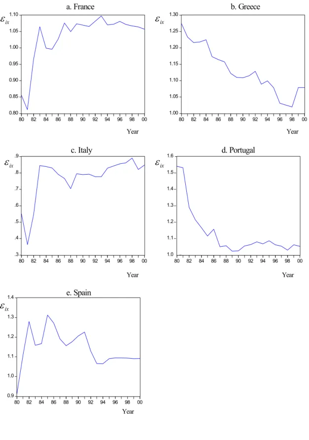
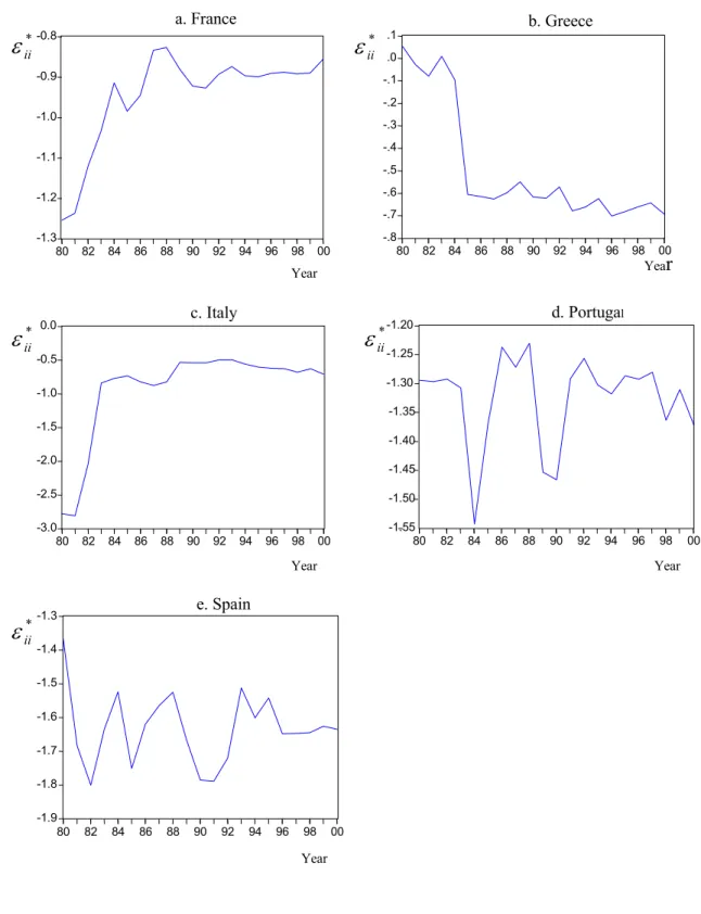
estimation of the whole system using the Kalman filter is not possible, and therefore estimation of the homogeneity-and-symmetry-restricted TVP-LAIDS models is beyond the context of this paper. However, with no restriction put on the parameters, it is feasible and valid to estimate the unrestricted TVP-LAIDS models equation by equation (Deaton and Muellbauer, 1980). Both unrestricted TVP-LR-LAIDS and TVP-EC-LAIDS are estimated using the Kalman filter algorithm. Tables 6 and 7 refer to the most up-to-date estimates of and , respectively. Evolutions of expenditure and own-price elasticities over time are plotted in Figs. 1 and 2
*
T
Π Π ∆
T
3 based on the estimates of the unrestricted TVP-LR-LAIDS.
(Insert Tables 6-7 here)
(Insert Figures 1 and 2 here).
With regard to expenditure elasticities (see Fig. 1), the most dramatic variations appeared in the early 1980s in almost all destinations except for Greece. During that period of time, expenditure elasticities for France, Italy and Spain underwent sharp increases, while the opposite situation is shown in Portugal. By contrast, since the mid 1980s the variations have become relatively mild. In the case of Greece, expenditure elasticities have been declining gradually throughout the whole observation period. On the other hand, the expenditure elasticity for Spain has experienced the most obvious fluctuations. Dritsakis (2004) found the same evidence when he examined the demand for Greek tourism by UK residents. In the case of Spain, after experiencing large variations before the 1990s, UK residents’ preferences have become relatively stable over the last decade. With respect to own-price elasticities (see Fig. 2), in a similar manner to expenditure elasticities, relatively large upturns or
3 Since the diffuse initialisation in the Kalman filter algorithm consumes a few observations at the
downturns took place in the early 1980s. These phenomena were associated with the global economic recession during this period. Either similar or opposite changing trends reflected the interrelationships between these destinations (substitutes or complements). Since the mid 1980s, gradual evolutions of own-price elasticities have been observed in France, Greece and Italy. Portugal and Spain, however, still exhibited large variations, with the influence of the Gulf War in the early 1990s being evident.
3.3. Comparisons of Forecasting Performance
Although the TVP-LAIDS allows one to examine the time varying characteristics of the coefficients in the demand model, the reasons why the parameters in the demand model vary over time in different manners remains unclear. However, the most important contribution of the TVP technique to econometrics is its ability to generate accurate forecasts. The forecasting performance of the TVP-LAIDS models, compared with the fixed-parameter counterparts, is a further concern of this study. Various fixed-parameter and TVP LAIDS models, in both long-run and error-correction forms, with and without restrictions, are included in the forecasting assessment, with the conventional unrestricted fixed-parameter long-run LAIDS being used as the benchmark. All of these models are re-estimated using the data up to 1996 and the observations over 1997-2000 are used to measure the one-year- to four-years-ahead forecasting accuracy. Forecasting errors for both w and are calculated in each model in order to examine these models’ abilities to forecast tourism demand (in terms of the expenditure share) levels and changes against the previous period. The error measures used for the forecasting comparison are the mean absolute percentage error (MAPE) and root mean square percentage error
(RMSPE) for demand levels, and MAE and RMSE for demand changes (see Witt and Witt 1992, Chapter 6 for justification).
The forecast results (see Table 8) suggest that in 90% of cases the TVP versions of the LAIDS models generate more accurate forecasts than their FP counterparts. The comparison between each pair of the EC-LAIDS and long-run LAIDS models shows that the former generally yields more accurate forecasts than the latter, with the only exception being the comparison between the unrestricted TVP-LR-LAIDS and unrestricted TVP-EC-LAIDS in terms of demand level forecasts. The superior performance of the EC-LAIDS is particularly evident when demand change forecasting is concerned, as all EC-LAIDS models are ranked ahead of the static/long-run LAIDS. This is reasonable since incorporating the error correction mechanism into the LAIDS specification contributes to capturing better the short-term demand variations. Comparing the overall performance with the benchmark unrestricted fixed-parameter long-run LAIDS, all of the specific LAIDS models except the homogeneity-and-symmetry-restricted fixed-parameter long-run LAIDS show improved forecasting accuracy, irrespective of whether demand levels or demand changes are being forecast. The poor performance of the homogeneity-and-symmetry-restricted fixed-parameter long-run LAIDS is associated with its misspecification, indicated by the failures of restriction tests. The overall evaluation across all models suggests, with regard to forecasting demand levels, the TVP version models (the unrestricted TVP-LR-LAIDS and the unrestricted TVP-EC-LAIDS) outperform all the other fixed-parameter counterparts, with 28.2% (or 20.7%) and 23.3% (or 20.0%) improvements of forecasting accuracy measured by RSMPE (or MAPE) being achieved, respectively, relative to the benchmark.
As far as demand changes are concerned, fixed-parameter homogeneous and symmetric EC-LAIDS performs the best in general, followed by the unrestricted TVP-EC-LAIDS. The superior performance of the homogeneity-and-symmetry-restricted fixed-parameter EC-LAIDS indicates that with appropriate theoretical restrictions imposed on the correctly specified model (incorporating the error correction mechanism), the forecasting ability of LAIDS is very likely to be improved. The TVP version of the homogeneous and symmetric EC-LAIDS is not available in this study, but examination of its forecasting performance certainly would be of interest of future research. Without considering short-run adjustments, the other TVP-LAIDS, the unrestricted TVP-LR-LAIDS, does not outperform any EC-LAIDS when forecasting demand changes, but appears to be the best amongst all three long-run LAIDS. Compared to the benchmark, the homogeneity-and-symmetry-restricted fixed-parameter EC-LAIDS and the unrestricted TVP-EC-LAIDS show the most significant improvements in overall forecasting accuracy, reducing forecast errors by 60.7% (or 54.7%) and 53.5% (or 49.8%) respectively, in terms of the MAE (or RSME).
When different forecasting horizons are considered, more insights can be noted. In terms of demand level forecasts, the homogeneity-and-symmetry-restricted fixed-parameter EC-LAIDS is ranked top over the one-year-ahead time horizon, followed by TVP-EC-LAIDS. The relatively low rank of the unrestricted TVP-LR-LAIDS results from its poor performance in the Portugal equation, although its performance in other equations is satisfactory. As the time horizon increases, the superiority of the unrestricted TVP-LR-LAIDS increases considerably and consistently, being ranked top in the two-years- and three-years-ahead forecasts and second in the four-years-ahead forecasts. The performance of the unrestricted TVP-EC-LAIDS appears more
stable, always being ranked second or third. The unrestricted fixed-parameter EC-LAIDS also shows its outstanding performance in the four-years-ahead case. The improvements in forecast accuracy of the two TVP-LAIDS models relative to the benchmark can be seen throughout all horizons, with only one exception. The most remarkable improvement is seen in the one-year-ahead forecast, where the unrestricted TVP-EC-LAIDS and unrestricted TVP-LR-LAIDS generate 47.9% (or 40.1%) and 38.7% (or 29.1%) more accurate results, respectively, measured by RMSPE (or MAPE).
With respect to demand change forecasts, all of the models perform highly consistently across different horizons. Slight changes in rankings occur at the one-year-ahead prediction, in which the unrestricted TVP-EC-LAIDS outperforms the homogeneity-and-symmetry-restricted fixed-parameter EC-LAIDS, while on other occasions, the latter always performs the best amongst all competitors. Unlike demand level forecasts, the unrestricted TVP-EC-LAIDS gives the greatest improvements of demand change forecast accuracy at three-years- and four-years-ahead forecasting horizons, with increases in forecast accuracy of up to 70%.
4. Summary and Conclusions
In this study, various LAIDS models have been compared in terms of model specifications and forecasting performance, using data on the demand for Western European tourism by UK residents. The theoretical restriction tests suggest that the dynamic LAIDS incorporating the error correction mechanism is the most appropriate functional form. The Kalman filter estimates of the TVP-LAIDS models provide a clear illustration of the evolution of demand elasticities over time. The superiority of the TVP-LAIDS models’ performance is observed, for the present set of data, in terms
of the improvement of forecasting accuracy compared with the conventional unrestricted fixed-parameter long-run LAIDS, especially in the short term.
The forecasting assessment shows that the introduction of TVPs into the LAIDS has greatly improved the forecasting performance. Both the unrestricted TVP-LR-LAIDS and the TVP-EC-TVP-LR-LAIDS outperform the other FP competitors according to one-year- to four-years-ahead forecasting in terms of demand levels. The unrestricted TVP-EC-LAIDS also shows improved forecasting performance in terms of demand changes. In addition, incorporating the short-run adjustment mechanism into the LAIDS can increase forecasting accuracy, especially when demand change forecasting is concerned.
The empirical results in this paper support those of previous tourism demand studies which have also employed TVP models (Riddington, 1999; Song et al, 2003; Song and Witt, 2000). So far TVP models have generally performed well in modelling and forecasting tourism demand. Its further combinations with other advanced econometric approaches should be considered for applications in this field.
Due to a lack of sufficient observations available for this study, a complete illustration of the superiority of the TVP-LAIDS models under theoretical restrictions has not been possible. Since this study has shown the superior forecasting performance of the homogeneity-and-symmetry-restricted fixed-parameter EC-LAIDS, the predictive ability of its TVP counterpart remains an area for further investigation.
References
Alston, J. M., K. A. Foster and R. D. Green (1990). Estimating Elasticities with the Linear Approximate Almost Ideal Demand System: Some Monte Carlo Results. The Review of Economics and Statistics, 76, 351-356.
Anderson, G. and R. Blundell (1983). Testing Restrictions in a Flexible Dynamic Demand System: An Application to Consumers’ Expenditure in Canada. Review of Economic Studies 50, 397-410.
Attfield, C.L.F. (1997). Estimating a Cointegrating Demand System. European Economic Review, 41, 61-73.
Baldwin, M. A., M. Hadid and G. D. A. Phillips (1983). The Estimation and Testing of a System of Demand Equations for the UK, Applied Economics, 15, 81-90.
Belsley, D. A. (1973). On the Determination of Systematic Parameter Variation in the Linear Regression Model, Annals of Economic and Social Measurement, 2, 487-494.
Belsley, D. A. and E. Kuh (1973). Time-Varying Parameter Structures: An Overview, Annals of Economic and Social Measurement, 2, 375-379.
Blanciforti, L., R. Green and G. King (1986). U.S. Consumer Behaviour over the Post-war Period: An Almost Ideal Demand System Analysis, Monograph Number 40, Giannini Foundation of Agricultural Economics, University of California.
Buse, A. (1994). Evaluating the Linearized Almost Ideal Demand System, American Journal of Agricultural Economics, 76, 781-793.
Chambers, M. J. (1990). Forecasting with Demand Systems: A Comparative Study, Journal of Econometrics, 44, 363-376.
Chambers, M. J. and K. B. Nowman (1997). Forecasting with the Almost Ideal Demand System: Evidence from Some Alternative Dynamic Specifications, Applied Economics, 29, 935-943.
Cooley, T. F. and E. C. Prescott (1976). Estimation in the Presence of Stochastic Parameter Variation, Econometrica, 44, 167-183.
De Jong, P. (1991a). The Diffuse Kalman Filter, Annals of Statistics, 19, 1073-1083.
De Jong, P. (1991b). Stable Algorithms for State Space Model, Journal of Time Series Analysis, 12, 143-157.
De Mello, M., A. Pack and M. T. Sinclair (2002). A System of Equations Model of UK Tourism Demand in Neighbouring Countries, Applied Economics, 34, 509-521.
Deaton, A. S. and J. Muellbauer (1980). An Almost Ideal Demand System, American Economic Review, 70, 312-326.
Divisekera, S. (2003). A Model of Demand for International Tourism, Annals of Tourism Research, 30, 31-49.
Doran, H. E. and A. N. Rambaldi (1997). Applying Linear Time-varying Constraints to Econometric Models: With an Application to Demand Systems, Journal of Econometrics, 79, 83-95.
Duffy, M. (2002). Advertising and Food, Drink and Tobacco Consumption in the United Kingdom: A Dynamic Demand System, Agricultural Economics, 1637, 1-20.
Durbarry, R. and M. T. Sinclair (2003). Market Shares Analysis: The Case of French Tourism Demand, Annals of Tourism Research,30, 927-941.
Durbin, J. and S. J. Koopman (2001). Time Series Analysis by State Space Methods, Oxford University Press: New York.
Edgerton, D. L., B. Assarsson, A. Hummelmose, I. P. Laurila, K. Rickertsen and P. H. Vale (1996). The Econometrics of Demand Systems with Applications to Food Demand in the Nordic Countries, Kluwer Academic Publishers: London.
Engle, R. F. and C. W. J. Granger (1987). Cointegration and Error Correction: Representation, Estimation and Testing, Econometrica, 55, 251-276.
Fujii, E., M. Khaled and J. Mark (1985). An Almost Ideal Demand System for Visitor Expenditures, Journal of Transport Economics and Policy, 19, 161-171.
Green, R. and J. Alston (1990). Elasticities in AIDS Models, American Journal of Agricultural Economics, 72, 442-445.
Greenslade, J. V. and S. G. Hall (1996). Modelling Economies Subject to Structural Change: The Case of Germany, Economic Modelling, 13, 545-559.
Harvey, A. C. (1989). Forecasting, Structural Time Series Models and the Kalman Filter. Cambridge University Press: Cambridge.
Johansen, S. (1988). A Statistical Analysis of Cointegration Vectors. Journal of Economic Dynamics and Control, 12, 231-254.
Judge, G. G., W. E. Griffiths, R. Carter-Hill, H. Lütkepohl, and T. C. Lee (1985). The Theory and Practice of Econometrics, Second Edition, Wiley: New York.
Kalman, R. E. (1960). A New Approach to Linear Filtering and Prediction Problems, Transitions ASME, Journal of Basic Engineering, 82, 35-45.
Karagiannis, G. and G. J. Mergos (2002). Estimating Theoretically Consistent Demand Systems Using Cointegration Techniques with Application to Greek Food Data, Economics Letters, 74, 137-143.
Karagiannis, G. and K. Velentzas (1997). Explaining Food Consumption Patterns in Greece, Journal of Agricultural Economics, 48, 83-92.
Karagiannis, G., S. Katranidis and K. Velentzas (2000). An Error Correction Almost Ideal Demand System for Meat in Greece, Agricultural Economics, 22, 29-35.
Lucas, R. E. (1976). Econometric Policy Evaluation: A Critique, in K. Brumer and A. H. Meltzer (eds), The Phillips Curve and Labour Markets, Carnegie Rochester Conference Series on Public Policy, Northlands, Amsterdam.
Lyssiotou, P. (2001). Dynamic Analysis of British Demand for Tourism Abroad, Empirical Economics, 15, 421-436.
O’Hagan, J. W. and M. J. Harrison (1984). Market Shares of US Tourism Expenditure in Europe: An Econometric Analysis, Applied Economics, 16, 919-931.
Papatheodorou, A. (1999). The Demand for International Tourism in the Mediterranean Region, Applied Economics, 31, 619-630.
Pollak, R. and T. Wales (1992). Demand System Specification & Estimation. University Press: Oxford.
Ramajo, J. (2001). Time-Varying Parameter Error Correction Models: The Demand for Money in Venezuela, 1983.I-1994.IV, Applied Economics, 33, 771-782.
Ray, R. (1985). Specification and Time Series Estimation of Dynamic Gorman Polar Form Demand Systems, European Economic Review, 27, 357-374.
Riddington, G. L. (1999). Forecasting Ski Demand: Comparing Learning Curve and Varying Parameter Coefficient Aroaches, Journal of Forecasting, 18, 205-214.
Saris, A. H. (1973). A Bayesian Aroach to Estimation of Time Varying Regression Coefficients, Annals of Economic and Social Measurement, 2, 501-523.
Song, H. and S. F. Witt (2000). Tourism Demand Modelling and Forecasting: Modern Econometric Aroaches, Pergamon: Oxford.
Song, H., S. F. Witt and T. C. Jensen (2003). Tourism Forecasting: Accuracy of Alternative Econometric Models, International Journal of Forecasting, 19, 123-141.
Song, H. and K. F. Wong (2003). Tourism Demand Modeling: A Time Varying Parameter Approach, Journal of Travel Research, 42 (1), 57-64.
Stone, J. R. N. (1954). Linear Expenditure Systems and Demand Analysis: An Application to the Pattern of British Demand, Economic Journal, 64, 511-527.
Syriopoulos, T. C. and M. T. Sinclair (1993). An Econometric Study of Tourism Demand: the AIDS Model of US and European Tourism in Mediterranean
Countries, Applied Economics, 25, 1541-1552.
Tucci, M. P. (1995). Time-Varying Parameters: A Critical Introduction, Structural Change and Economic Dynamics, 6, 237-260.
White, K. (1985). An International Travel Demand Model: US Travel to Western Europe, Annals of Tourism Research, 12, 529-545.
Witt, S. F. and C. A. Witt (1992). Modeling and Forecasting Demand in Tourism. Academic Press: London.
Zellner, A. (1962). An Efficient Method of Estimating Seemingly Unrelated Regressions and Test for Aggregation Bias, Journal of the American Statistical Association, 57, 348-368.
Biographies:
Gang LI is a lecturer in Economics at the University of Surrey, UK. His primary research interests are in the areas of econometric modelling and forecasting, with a particular focus on tourism demand forecasting. He has published papers in Journal of Travel Research and Tourism Economics.
Haiyan SONG is Chair Professor of Tourism in the School of Hotel and Tourism Management at The Hong Kong Polytechnic University. His research interests include applied econometrics and forecasting, with particular emphasis on the evaluation of different modelling and forecasting methodologies. He has published articles in such academic journals as Journal of Applied Econometrics, Journal of Transport Economics and Policy, Economic Modelling and Applied Economics, and has co-authored the book Tourism Demand Modelling and Forecasting: Modern Econometric Approaches (2000).
Stephen WITT is a Visiting Professor in the School of Hotel and Tourism Management at The Hong Kong Polytechnic University, and is an Emeritus Professor at the University of Surrey, UK. His major research interests are econometric modelling of international tourism demand, and assessment of the accuracy of different forecasting methods within the tourism context. He has published 130 journal articles and book chapters, as well as 16 books including Modeling and Forecasting Demand in Tourism (1992), Tourism Demand Modelling and Forecasting: Modern Econometric Approaches (2000), Tourism Forecasts for Europe 2001– 2005 (2001) and Asia Pacific Tourism Forecasts 2005– 2007 (2005).
Table 1
Estimates of the long-run parameters in the unrestricted fixed-parameter long-run LAIDS
France Greece Italy Portugal Spain
logp1 0.023 (0.066) -0.031 (0.060) 0.049 (0.037) -0.054 (0.030) 0.055 (0.103) logp2 -0.044 (0.047) -0.133** (0.042) 0.064* (0.026) 0.003 (0.021) -0.020 (0.073) logp3 -0.157** (0.025) -0.053* (0.023) -0.014 (0.014) 0.047** (0.011) 0.114** (0.039) logp4 0.079 (0.041) -0.019 (0.037) -0.030 (0.023) -0.022 (0.019) -0.068 (0.065) logp5 0.163** (0.032) 0.108** (0.056) -0.051** (0.018) 0.039** (0.015) -0.245** (0.050) logp6 -0.167** (0.062) 0.099* (0.056) -0.065 (0.035) 0.009 (0.028) 0.293** (0.096) ) / log(x P* 0.008* (0.003) 0.005 (0.003) -0.009** (0.002) 0.006** (0.002) 0.028** (0.005) 2 R 0.898 0.747 0.800 0.815 0.570 S.E. 0.010 0.009 0.006 0.005 0.016 DW 2.568 1.480 2.367 2.046 2.487 Notes: * and ** refer to 5% and 1% significance levels, respectively. Values in parentheses are standard
errors. S.E. stands for the standard error, and DW for the Durbin-Watson statistic for the autocorrelation test. The estimates of the other parameters are omitted due to space limits, but available from the authors upon request.
Table 2
Estimates of the short-run parameters in the unrestricted fixed-parameter EC-LAIDS
France Greece Italy Portugal Spain
∆logp1 0.095** (0.031) 0.053 (0.031) 0.056* (0.026) -0.033 (0.025) -0.096 (0.074) ∆logp2 -0.026 (0.028) -0.025 (0.027) 0.013 (0.023) 0.025 (0.022) -0.027 (0.066) ∆logp3 -0.101** (0.019) 0.063* (0.026) -0.002 (0.016) 0.053** (0.016) 0.149** (0.046) ∆logp4 0.064 (0.026) -0.040 (0.042) -0.034 (0.022) -0.020 (0.021) -0.033 (0.063) ∆logp5 0.017 (0.024) 0.068 (0.038) -0.034 (0.020) 0.019 (0.019) -0.163** (0.057) ∆logp6 -0.135** (0.040) -0.009 (0.016) -0.070* (0.034) -0.004 (0.031) 0.328** (0.091) ∆log(x/P*) 0.022** (0.006) 0.006 (0.010) -0.012* (0.005) 0.008 (0.005) 0.025 (0.015) 2 R 0.866 0.504 0.586 0.404 0.705 S.E. 0.006 0.008 0.005 0.005 0.014 DW 1.757 1.731 2.011 2.113 1.699 Notes: As for Table 1.
Table 3
Restriction tests for homogeneity and symmetry
Model Homogeneity Symmetry Homogeneity and symmetry
Static LAIDS 2.259* 3.461 3.066
EC-LAIDS 2.236* 1.940* 1.962**
Table 4
Estimates of the long-run parameters in the homogeneity-and-symmetry-restricted fixed-parameter long-run LAIDS
France Greece Italy Portugal Spain
) / log(p1 p6 -0.019 (0.066) -0.019 (0.030) -0.091** (0.024) 0.003 (0.022) 0.202** (0.055) ) / log(p2 p6 -0.019 (0.030) -0.126** (0.025) -0.017 (0.015) -0.001 (0.014) 0.019 (0.032) ) / log(p3 p6 -0.091** (0.024) -0.017 (0.015) 0.027 (0.018) 0.029** (0.009) -0.005 (0.031) ) / log(p4 p6 0.003 (0.022) -0.001 (0.014) 0.029** (0.009) -0.013 (0.013) -0.018 (0.017) ) / log(p5 p6 0.202** (0.055) 0.019 (0.032) -0.005 (0.031) -0.018 (0.017) -0.311** (0.088) ) / log(x P* 0.010* (0.005) 0.013** (0.003) -0.015** (0.003) 0.011** (0.002) 0.029** (0.008) 2 R 0.774 0.737 0.544 0.802 0.160 S.E. 0.015 0.010 0.010 0.005 0.025 DW 1.495 1.468 1.261 1.976 1.540 Notes: As for Table 1.
Table 5
Estimates of the short-run parameters in the homogeneity-and-symmetry-restricted fixed-parameter EC-LAIDS
France Greece Italy Portugal Spain
∆ log(p1/ p6) (0.030) 0.034 -0.017 (0.021) -0.025 (0.017) 0.035 (0.019) 0.055 (0.032) ∆log(p2 /p6) -0.017 (0.021) -0.074* (0.030) -0.017 (0.015) 0.037* (0.017) 0.0003 (0.031) ∆log(p3/p6) -0.025 (0.017) -0.017 (0.015) 0.074** (0.017) 0.003 (0.026) -0.021 (0.026) ∆log(p4 /p6) 0.035 (0.019) 0.037* (0.017) 0.003 (0.026) -0.041* (0.019) 0.005 (0.021) ∆log(p5/ p6) 0.055 (0.032) 0.0003 (0.031) -0.021 (0.026) 0.005 (0.021) -0.215** (0.070) ∆log(x/P*) 0.033** (0.008) 0.018* (0.008) -0.003 (0.007) 0.003 (0.006) 0.006 (0.018) 2 R 0.678 0.471 -0.037 -0.049 0.439 S.E. 0.009 0.008 0.008 0.006 0.019 DW 1.646 2.101 1.501 1.781 1.770 Notes: As for Table 1.
Table 6
Kalman filter estimates of the long-run parameters in the final unrestricted TVP-LR-LAIDS model
France Greece Italy Portugal Spain
logp1 0.034 (0.049) 0.041 (0.029) 0.060* (0.025) -0.071** (0.020) 0.274** (0.034) logp2 -0.093 (0.063) 0.023 (0.037) 0.037 (0.031) 0.011 (0.025) 0.022 (0.136) logp3 -0.076 (0.052) -0.080** (0.031) 0.021 (0.026) 0.020 (0.021) -0.039 (0.043) logp4 0.092 (0.049) -0.034 (0.029) -0.063* (0.025) -0.015 (0.020) -0.179** (0.031) logp5 0.047 (0.056) 0.084* (0.033) -0.022 (0.028) 0.036 (0.023) -0.170** (0.062) logp6 -0.103 (0.081) -0.058 (0.048) -0.083* (0.040) 0.020 (0.033) 0.125 (0.068) ) / log(x P* 0.012 (0.010) 0.006 (0.006) -0.012* (0.005) 0.002 (0.004) 0.026** (0.004) Log likelihood 43.112 54.132 57.722 62.058 36.966 AIC -2.146 -2.057 -3.153 -3.452 -1.722 NO(2) 0.167 0.043 0.425 0.304 1.308 HE(7, 7) 3.500 8.738** 3.351 3.359 4.706* PF(4, 17) 0.221 0.705 1.033 0.709 0.016
Notes: As for Table 1. In addition, NO(2) is a normality test, HE(7, 7) is a heteroscedasticity test, PF(4, 22) is a post-sample predictive failure test, with values in brackets denoting degrees of freedom. Details of these tests can be seen in Harvey (1989).
Table 7
Kalman filter estimates of the short-run parameters in the final unrestricted TVP-EC-LAIDS model
France Greece Italy Portugal Spain
∆logp1 0.1522** (0.041) 0.026 (0.033) 0.060** (0.021) -0.034 (0.020) -0.048 (0.051) ∆logp2 -0.034 (0.025) -0.033 (0.036) 0.019 (0.022) 0.025 (0.022) -0.013 (0.054) ∆logp3 -0.106** (0.021) -0.057* (0.028) 0.003 (0.018) 0.055** (0.019) 0.135** (0.051) ∆logp4 0.081** (0.022) -0.017 (0.033) -0.040* (0.020) -0.019 (0.019) -0.053 (0.049) ∆logp5 0.014 (0.021) 0.055 (0.031) -0.031 (0.019) 0.017 (0.018) -0.157** (0.048) ∆logp6 -0.160** (0.029) 0.027 (0.043) -0.077** (0.027) -0.002 (0.027) 0.277 (0.157) ∆log(x/P*) 0.021** (0.007) 0.010 (0.009) -0.013* (0.006) 0.008 (0.006) 0.039* (0.016) Log likelihood 63.759 57.257 67.285 68.752 45.955 AIC -3.697 -3.233 -3.949 -4.504 -2.425 NO(2) 2.729 0.156 7.179** 0.433 1.161 HE(7, 7) 9.807** 9.388** 7.598** 3.786 2.316 PF(4, 17) 0.369 0.835 1.182 0.440 0.085
Table 8
Comparisons of forecasting accuracy of various LAIDS models over different forecasting horizons
Horizon Measure U-FP-LR-LAIDS U-TVP-LR-LAIDS U-FP-EC-LAIDS U-TVP-EC-LAIDS H&S-FP-LR-LAIDS H&S-FP-EC-LAIDS 1 year MAPE 0.103 (5) 0.079 (4) 0.063 (3) 0.061 (2) 0.146 (6) 0.058 (1) RSMPE 0.163 (5) 0.108 (4) 0.090 (3) 0.085 (2) 0.178 (6) 0.082 (1) 2 years MAPE 0.120 (5) 0.091 (1) 0.114 (4) 0.103 (2) 0.175 (6) 0.107 (3) RSMPE 0.199 (5) 0.131 (1) 0.163 (4) 0.150 (2) 0.213 (6) 0.151 (3) 3 years MAPE 0.128 (3) 0.119 (1) 0.166 (5) 0.124 (2) 0.168 (6) 0.134 (4) RSMPE 0.170 (3) 0.143 (1) 0.215 (6) 0.165 (2) 0.190 (5) 0.173 (4) 4 years MAPE 0.207 (5) 0.156 (2) 0.118 (1) 0.161 (3) 0.216 (6) 0.178 (4) RSMPE 0.261 (6) 0.186 (2) 0.142 (1) 0.197 (3) 0.245 (5) 0.212 (4) Overall MAPE 0.140 (5) 0.111 (1) 0.115 (3) 0.112 (2) 0.176 (6) 0.119 (4) RSMPE 0.202 (5) 0.145 (1) 0.159 (3) 0.155 (2) 0.208 (6) 0.162 (4) 1 year MAE 7.427 (5) 6.536 (4) 5.208 (3) 4.908 (1) 14.166 (6) 5.008 (2) RSME 10.021 (5) 8.122 (4) 6.236 (2) 6.019 (1) 15.725 (6) 6.588 (3) 2 years MAE 7.460 (6) 7.137 (5) 5.306 (3) 4.372 (2) 63924 (4) 3.837 (1) RSME 9.210 (6) 8.866 (5) 6.310 (3) 5.855 (2) 7.781 (4) 5.110 (1) 3 years MAE 7.995 (5) 8.930 (6) 5.121 (3) 2.389 (2) 7.039 (4) 1.801 (1) RSME 9.897 (5) 10.359 (6) 6.029 (3) 2.915 (2) 7.782 (4) 2.205 (1) 4 years MAE 8.890 (6) 8.183 (5) 3.426 (3) 3.115 (2) 5.900 (4) 1.850 (1) RSME 10.287 (6) 9.960 (5) 4.479 (3) 4.360 (2) 5.912 (4) 2.367 (1) Overall MAE 7.943 (5) 7.696 (4) 4.765 (3) 3.696 (2) 8.507 (6) 3.124 (1) RSME 9.862 (5) 9.369 (4) 5.812 (3) 4.950 (2) 10.063 (6) 4.471 (1) Notes: The upper half of the table refers to the forecasts of levels variables, and the lower to differenced variables. The unit of the figures in the lower half of the table is
ix
ε
ixε
ixε
ε
ix ixε
0.80 0.85 0.90 0.95 1.00 1.05 1.10 80 82 84 86 88 90 92 94 96 98 00 a. France 1.00 1.05 1.10 1.15 1.20 1.25 1.30 80 82 84 86 88 90 92 94 96 98 00 b. Greece .3 .4 .5 .6 .7 .8 .9 80 82 84 86 88 90 92 94 96 98 00 c. Italy 1.0 1.1 1.2 1.3 1.4 1.5 1.6 80 82 84 86 88 90 92 94 96 98 00 d. Portugal 0.9 1.0 1.1 1.2 1.3 1.4 80 82 84 86 88 90 92 94 96 98 00 e. Spain Year Year Year Year YearFig. 1 Kalman filter estimates of expenditure elasticities (εix) in the unrestricted TVP-LR-LAIDS (1980-2000)
-1.3 -1.2 -1.1 -1.0 -0.9 -0.8 80 82 84 86 88 90 92 94 96 98 00 a. France -.8 -.7 -.6 -.5 -.4 -.3 -.2 -.1 .0 .1 80 82 84 86 88 90 92 94 96 98 00 b. Greece -3.0 -2.5 -2.0 -1.5 -1.0 -0.5 0.0 80 82 84 86 88 90 92 94 96 98 00 c. Italy -1.55 -1.50 -1.45 -1.40 -1.35 -1.30 -1.25 -1.20 80 82 84 86 88 90 92 94 96 98 00 d. Portugal -1.9 -1.8 -1.7 -1.6 -1.5 -1.4 -1.3 80 82 84 86 88 90 92 94 96 98 00 e. Spain Year Year Year Year Year * ii
ε
* iiε
* iiε
* iiε
* iiε
Fig. 2 Kalman filter estimates of compensated own-price elasticities ( ) in the unrestricted TVP-LR-LAIDS (1980-2000)
*
ii