Improving forecasting accuracy of crude oil price using decomposition ensemble model with reconstruction of IMFs based on ARIMA model

Improving forecasting accuracy of crude oil price using

decomposition ensemble model with reconstruction of IMFs based

on ARIMA model

Muhammad Aamir

, Ani Shabri

, Muhammad Ishaq

a _{Department of Mathematical Sciences, Faculty of Science, Universiti Teknologi Malaysia, Skudai 81310, Johor, Malaysia} b _{School of Natural Sciences, National University of Sciences and Technology, Islamabad, Pakistan}

c _{Department of Statistics, Abdul Wali Khan University Mardan, Pakistan} * Corresponding author: [email protected]

Article history

Received 31 January 2018 Revised 22 Mac 2018 Accepted 12 June 2018

Published Online 3 December 2018 Graphical abstract

Input

EEMD

IMF 1 IMF 2 IMF 3 … IMF k

Order of ARIMA model Order of ARIMA model Order of ARIMA model Order of ARIMA model … IMFs Reconstruction

IMF 1 IMF 2 IMF 3 … IMF k-n

ARIMA Forecasting model ARIMA Forecasting model ARIMA Forecasting model ARIMA Forecasting model … ∑

Prediction Results Prediction Results

Output

Abstract

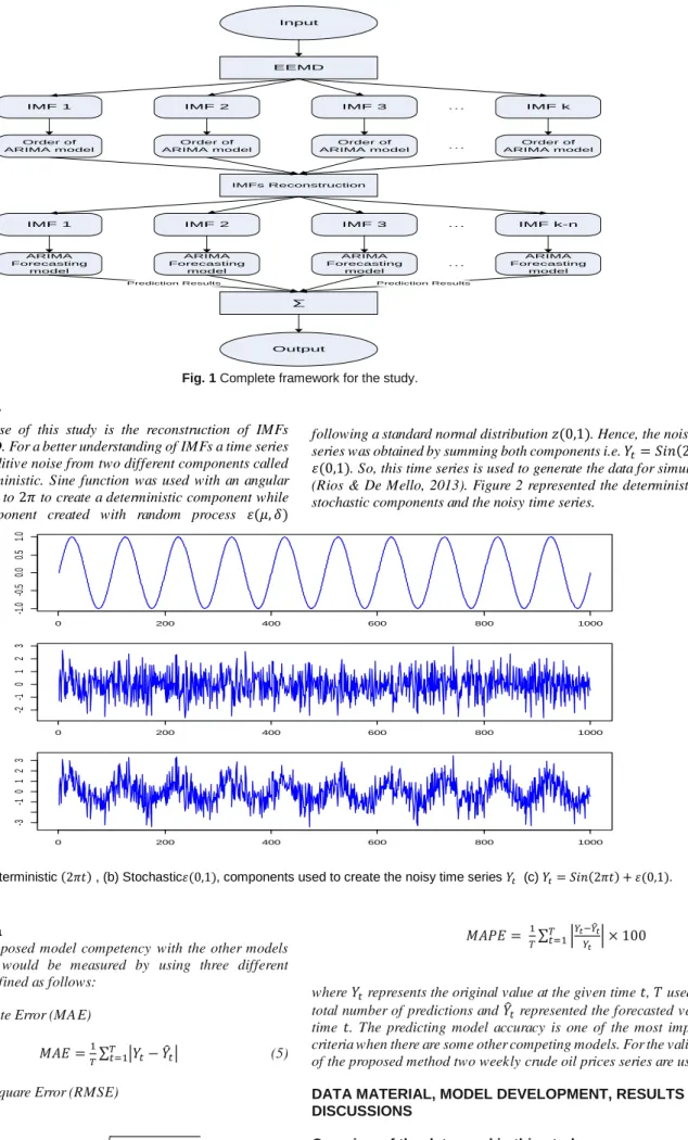
The accuracy of crude oil price forecasting is more important especially for economic development and considered as the lifeblood of the industry. Hence, in this paper, a decomposition-ensemble model with the reconstruction of intrinsic mode functions (IMFs) is proposed for forecasting the crude oil prices based on the well-known autoregressive moving average (ARIMA) model. Essentially, the reconstruction of IMFs enhances the forecasting accuracy of the existing decomposition ensemble models. The proposed methodology works in four steps: decomposition of the complex data into several IMFs using EEMD, reconstruction of IMFs based on order of ARIMA model, prediction of every reconstructed IMF, and finally ensemble the prediction of every IMF for the final output. A case study was carried out using two crude oil prices time series (i.e. Brent and West Texas Intermediate (WTI)). The empirical results exhibited that the reconstruction of IMFs based on order of ARIMA model was adequate and provided the best forecast. In order to check the correctness, robustness and generalizability, simulations were carried out.

Keywords: ARIMA, crude oil, EEMD, forecasting, reconstruction

© 2018 Penerbit UTM Press. All rights reserved

INTRODUCTION

Oil is treated as the main energy source for economic development and lifeblood for industries. Unsurprisingly, most of the macroeconomic variables forecasts rely on the changes in crude oil prices like inflation. Furthermore, the price of crude oil futures heavily depends on past crude oil prices. However, in recent years the future of crude oil prices is very uncertain and very hard to quantify because of irregular events, speculation activities, global economic status, political and social activities. Therefore, forecasting the crude oil prices gain a considerable amount of attention from an academician, investors and government agencies. Thus, this paper concentrates on forecasting crude oil prices to examine the hidden components which caused the model execution as far as forecast accuracy and time.

The current literature consisting of several time-series forecasting models which have been used for forecasting the world crude oil prices. The existing time series models can fall into three broader categories:

random walk (RW), error correction model (ECM), generalized autoregressive conditional heteroscedasticity (GARCH) and vector auto-regression (VAR) models. Afterwards are the AI techniques which proved their superiority on the econometric models with the help of empirical investigations for forecasting the crude oil prices the most dominant techniques among the AI are artificial neural network (ANN) and least square support vector regression (LSSVR). However, nowadays the third type of models are widely used for forecasting the world crude oil prices. These models work under the concept of decomposition and ensemble (Wang et al., 2005) and predominant techniques used for forecasting crude oil prices are empirical mode decomposition (EMD), EEMD and wavelet transformation (WT).

ARIMA model was used by (Xiang and Zhuang, 2013) to predict short-term Brent crude oil prices for the period spanning Nov 2012 to Apr 2013. GARCH family models were also used by (Nomikos and Andriosopoulos, 2012) for forecasting the crude oil prices and estimated the volatility and conditional mean of WTI daily data

Aamir et al. / Malaysian Journal of Fundamental and Applied Sciences Vol. 14, No. 4 (2018) 471-483 for forecasting the monthly WTI prices for the data from May 1987 to

Dec 2011. SVR model was utilized for forecasting the monthly WTI prices for the data from Jan 1970 to Dec 2003 in addition (Xie et al., 2006) also proved that SVR model outperforms back-propagation neural network (BPNN) and the well-known ARIMA models. SVR model was also used by (Khashman & Nwulu, 2011) and forecasted crude oil prices of WTI over the period spanning Jan 1986 to Dec 2009. LSSVR model was incorporated by (Li et al., 2013) and forecasted weekly crude oil prices of WTI for a period spanning Jan 4, 2008, to Oct 18, 2013, and made a conclusion that LSSVR model performed better than SVR, BPNN, and well-known ARIMA models. However, these models have their own shortcomings, in conventional econometric models the problem of stationarity and linearity while in AI models the problem of sensitiveness in parameters and overfitting.

Subsequently, next is the hybrid models which work with the idea of decomposition and ensemble. Decomposition and ensemble paradigms are very popular among researchers in recent time and very common in practice for forecasting the crude oil prices. The typical decomposition ensemble paradigms consist of three steps: simplification of complex data into different components, forecasting the individual components, and ensemble all forecasting components for final forecasting (Liu et al., 2013; Tang et al., 2012; Yu et al., 2008). The decomposition ensemble paradigms proved their superiority by producing low forecasting error or in other words, enhanced the forecasting accuracy. EMD model was incorporated by Yu et al., (2008) for forecasting the Brent and WTI daily crude oil prices and produced better results as compared to the traditional models, the data used in the study spanning May 20, 1987 to Sep 30, 2006 and Jan 01, 1986 to Sep 30, 2006 respectively. Complementary ensemble EMD technique used by Tang et al., (2015) for forecasting the crude oil prices and the results demonstrated that the decomposition ensemble strategy is a better technique which enhanced forecasting accuracy. A novel learning paradigm was introduced by Yu et al., (2016) based on EEMD with an extended extreme learning machine for forecasting the WTI crude oil prices over the period spanning Jan 02, 1986 to Oct 21, 2013. All the studies proved that the decomposition and ensemble strategy is a better procedure for forecasting the crude oil prices.

The complex data of crude oil prices effectively handled by hybrid decomposition ensemble models as compared to the non-hybrid models. However, an important issue arises of computational cost and model complexity. Because at the decomposition stage the original series be decomposed into components and modelled the individual series may consume more time and sometimes produced poor results. To solve this issue of an individual model, an additional step of reconstruction of IMFs would be introduced before modelling and forecasting the individual IMFs. In the reconstruction step, some of the IMFs combined with other IMFs for further analysis before the individual modelling of each IMF.

Recently, some studies have been carried out on IMFs reconstruction concept which assured the importance of this technique. For example, EMD modes have been reconstructed by Shu-ping et al., (2014) into high, medium, low frequencies and in a trend sequence through run-length judgment method, this novel technique outperformed the decomposition ensemble results without reconstruction of IMFs in forecasting the crude oil prices. Yan et al., (2014) also reconstructed the EMD modes into groups by the method of fine-to-coarse for forecasting the uranium prices. Based on the sample entropy measurement the decomposed modes be reconstructed for wind speed data and a similar conclusion has been drawn (G. Zhang et al., 2014). EEMD paradigm modes was reconstructed by (Yu et al., 2015) by using the “data-characteristic-driven” approach, the main data characteristics were data complexity (i.e. high and low) and pattern characteristics (i.e. cyclicity, mutability, and tendency), the empirical results showed that the reconstruction of modes enhanced the forecasting accuracy for both WTI and Brent weekly crude oil prices covering periods from Jan 03, 1986 to Jul 11, 2014, and Jan 01, 1986 to Jul 11, 2014, respectively lastly Aamir and Shabri (2018) also reconstructed the EEMD modes into stochastic and deterministic components which enhanced the forecasting accuracy. In the above reconstruction of IMFs studies, they conducted the reconstruction of the modes based on some data characteristics i.e. average, frequency or

complexity. To effectively capture some significant inner hidden factors of the decomposed IMFs a strong and simple analysis of the reconstruction of IMFs are strongly recommended.

Under such a foundation, this paper aims to enhance the forecasting power of current decomposition ensemble models, particularly through reconstructions of IMFs. The proposed procedure for reconstruction of IMFs is the order of the ARIMA model. The reason behind the use of the order of ARIMA model is that, that after the first few IMFs there is no autoregressive pattern left in the rest of the IMFs, some of them follow the random walk pattern and some are deterministic curves. Thus, from this point, we got the motivation and wanted to focus on this issue. The proposed technique is very simple and comparatively less time consuming which significantly enhanced the forecasting accuracy of the crude oil prices. Based on the idea of reconstruction of IMFs through the order of the ARIMA model is interesting because to the best of our knowledge there is no model used to reconstruct the IMFs through a model. All previous techniques based on the data characteristics. The academic contribution of this study is the enhancement of the forecasting accuracy of the crude oil prices by putting less labor and getting more. The second advantage of this study is to consider another decomposition model as well by reconstructing their modes for better forecasting. The third contribution of the proposed reconstructing method is the simplification of the model selection for the new modes.

For illustration and validation purpose, the two well-known crude oil prices were used as sample i.e. Brent and WTI. For comparison purposes, the most popular single ARIMA model, decomposition ensemble model without reconstruction of IMFs and other methods of reconstruction of IMFs were used as benchmark models. To check the correctness, robustness and generalizability of the proposed reconstruction of IMFs method simulations were also carried out. The rest of the paper is organized as follows: Section 2 describes the methodologies used in this study. Section 3 describes the data material, model development, real-world application, simulations, discussion, and results. The last section 4 concludes the paper and outline the future research work direction.

METHODS USED IN THE STUDY ARIMA model

The most popular procedure in the field of univariate time series analysis is Box-Jenkins ARIMA models (Montgomery et al., 2013) was introduced by Box and Jenkins (1976). In the last 50 years, this procedure has become very common and it is frequently used for forecasting the time series applications. The autoregressive (AR) and moving average (MA) models originate the ARIMA model. The current value of the time series using the AR model based on the pth_previous

values of the time series can be expressed as follows:

𝑌𝑡= 𝜃0+ 𝜃1𝑌𝑡−1+ 𝜃2𝑌𝑡−2+ ⋯ + 𝜃𝑝𝑌𝑡−𝑝+ 𝜇𝑡 (1)

The MA model of order q modelled the random error. The current value of the time series is expressed as the current error at time t and qth

previous values of the random error in the following formula.

𝑌𝑡= 𝜇𝑡− ∅1𝜇𝑡−1− ∅2𝜇𝑡−2− ⋯ − ∅𝑞𝜇𝑡−𝑞 (2)

The combined expression of AR and MA model makes the ARMA (p,q) process defined as follows:

𝑌𝑡= 𝜃0+ 𝜃1𝑌𝑡−1+ 𝜃2𝑌𝑡−2+ ⋯ + 𝜃𝑝𝑌𝑡−𝑝+ 𝜇𝑡− ∅1𝜇𝑡−1−

∅2𝜇𝑡−2− ⋯ − ∅𝑞𝜇𝑡−𝑞 (3)

where 𝑌𝑡 is the observed or predicted value at time 𝑡, 𝑌𝑡−𝑗 are the

observed previous values, 𝜃𝑗 are the coefficients of the previously

observed time series values, ∅𝑗 are the coefficients of the previous

white noises, 𝜇𝑡 is a white noise process normally distributed with zero

mean and 𝛿2 _{variance and 𝜇}

𝑡−𝑗 are used for the previous noise terms.

One of the strict assumptions of the ARMA model is stationarity, however, most of the time series is not stationary. To achieve

stationarity the time series is differenced dth _{time. In practice, the}

difference operator d is usually taken as 0, 1, or 2 (Box et al., 2015). Thus, the ARIMA model of order (p, d, q) are as follows:

𝜔𝑡= 𝜃1𝜔𝑡−1+ 𝜃2𝜔𝑡−2+ ⋯ + 𝜃𝑝𝜔𝑡−𝑝+ 𝜇𝑡− ∅1𝜇𝑡−1−

∅2𝜇𝑡−2− ⋯ − ∅𝑞𝜇𝑡−𝑞 (4)

where 𝜔𝑡= 𝛻𝑑𝑌𝑡. If 𝑑 = 0, then 𝜔𝑡= 𝑌𝑡 and equation (4) become an

ARMA model. The theoretical background and detailed description of the ARIMA model can be found in (Box et al., 2015).

The ensemble empirical mode decomposition

The new opportunities of extracting the time differing components from data have provided by Huang et al., (1999) after the development of the transient local and adaptive method of EMD. The transient locality is one of the most important characteristics of EMD, which is acquired from the spline fitting through the minima and maxima of inputted information. The spline fitting has high transient territory and can be effortlessly confirmed utilizing numerical programming. The transient territory of EMD is all around saved if the number of sifting is smaller and fixed. Both transient territory and amplitude recurrence balance of oscillatory segments is worse by the excessive use of the sifting process of EMD. The non-stationarity assumption of the data automatically bypasses by the temporal locality of EMD which is one of the advantages of this procedure. The EMD procedure has some unique properties: (a) For EMD no basis function is required because the decomposition procedure is fully adaptive (b) EMD is a highly effective decomposition procedure because it is a scanty approach and works like a dyadic channel bank (Flandrin et al., 2004; Wu and Huang, 2004, 2010) (c) For different signals, EMD accomplishes like a bank of spline wavelet of various orders (Flandrin and Goncalves, 2004; Wu and Huang, 2010) (d) EMD components of a given noise series share the same Fourier spectrum (except the first component) after rescaling amplitude and frequency (e) Everything except the primary EMD component of the noise follows normal distribution (Wu et al., 2016; Wu and Huang, 2004). Due to these interesting properties EMD naturally connects with the widely-used decomposition procedures like wavelet decomposition and Fourier spectrum-based filtering methods. The captivating possessions of EMD with extracting supremacy of physical information from data have eased a wide number of applications from different fields.

For the physical interpretability of the outcomes, EMD locality provides the necessary condition but not sufficient. However, analysing the non-stationary data there are different restrictions on the physical interpretability of the outcomes. Among these restrictions, one is the sensitivity of the outcomes of analysis due to the noise contained in data because in actual data set the noise is universal. On the off-chance that the outcomes are not sensitive to little but rather not tiny noise, they are for the most part considered physically interpretable; else, they are definitely not. The extracted components of EMD becomes highly sensitive to the extrema (minima) distribution. Tragically, without noise locations of data and the extrema (minima) values changed due to the unknowing non-stationary noise confined in the data. An EMD approach comprises of proceeding with levels of extricating oscillatory segments of lower recurrence, the noise twisted outcomes at one level can prompt proceeding with bending of consequent oscillatory parts, making EMD comes about barely physically interpretable. This absence of robustness brought about the inadequacy of EMD.

To conquer this robustness problem, several procedures have been adopted as (Huang et al., 1999) introduced the intermittency test. In such tests, variation in one component controlled, which leads to

reducing the adaptiveness calls for more compelling methodologies. EEMD method was introduced by Wu and Huang (2009), a noise-assisted data analysis technique which exactly fulfills the required challenge of robustness.

The steps involved in EEMD are as following: (a) in a first step a white noise series is added to the original time series𝑌𝑡; (b) after adding

the white noise decomposed the time series into components; (c) adding different white noise to the series and repeat step (a) and (b) again and again, and (d) obtained the ensemble means of the respective IMFs of the decompositions as the result. The white noise properties which are used by EEMD in these steps are: the distribution of maxima at any timescale be temporally uniform and EMD being effectively a twofold channel bank for white-noise (Flandrin et al., 2004; Wu and Huang, 2004, 2010). The distribution of the added white-noise on all timescales of extrema distribution is relatively even. The second property of the added white noise which is twofold filter bank takes control of the oscillatory component, which reduces the chance of scale mixing in a component significantly. As a result, the decomposition becomes more stable and physically meaningful.

Hybrid EEMD-ARIMA model

The procedure of hybrid EEMD-ARIMA modelling can be summarized in the following steps (Wang et al., 2015).

•The original time series be decomposed into 𝑘 components.

•For each 𝑘𝑡ℎ _{component choose the best ARIMA model and}

predict every component accordingly.

•Combined the output of all 𝑘 components for the targeted series. The main advantage of the decomposition and ensemble strategy is to simplify the task of predicting a series. The decomposed IMFs are easy to predict as compared to the original time series and additionally the forecasting accuracy is also improved. Which is one of the advantages of the decomposition and ensemble methodology? By hybridizing the two models ease the work at the computation stage and provided more efficient results because one issue is handled by one model and the other issue handled by the other model. That’s why hybridization is selected for best performance in this study.

The proposed methodology

In this study, the proposed methodology is the reconstruction of IMFs of EEMD. Firstly, the time series be decomposed into 𝑘 IMFs by EEMD. Next, choose the best order (𝑝, 𝑑, 𝑞) of ARIMA model for every 𝑘𝑡ℎ _{IMF based on the ACF, PACF graphs and for stationarity} Augmented Dickey-Fuller (ADF) is used. As by the definition of IMFs, the first IMF has a high-frequency modulation as compared to the next proceeding IMF while the last IMF be completely deterministic. The problem is where to fix the bench line or cut off point. As we know that the class of ARMA models could handle cyclic behaviour and seasonality of a time series. Whenever 𝑝 > 1 of an ARMA(𝑝, 𝑞) model means there should be some problem of cyclicity and seasonality. So, the basic idea of the reconstruction of IMFs in this study is to handle individually all IMFs where the problem of cyclicity and seasonality exist and combine all those IMFs where this problem is not existing. Thus, in this work, a simple, criterion is designed for the bench line IMF. After obtaining all IMFs check the order of ARIMA model starting from IMF_1 to IMF_k and combine all those IMFs who fulfil this condition 𝑝 ≤ 1. Thus, for further analysis, the number of IMFs to be used is (𝑘 − 𝑛 + 1), where 𝑛 is the number of IMFs which is combined and make one IMF. Figure 1 illustrate the complete framework of the proposed study.

Aamir et al. / Malaysian Journal of Fundamental and Applied Sciences Vol. 14, No. 4 (2018) 471-483

Input

EEMD

IMF 1 IMF 2 IMF 3 … IMF k

Order of ARIMA model Order of ARIMA model Order of ARIMA model Order of ARIMA model … IMFs Reconstruction

IMF 1 IMF 2 IMF 3 … IMF k-n

ARIMA Forecasting model ARIMA Forecasting model ARIMA Forecasting model ARIMA Forecasting model … ∑

Prediction Results Prediction Results

Output

Fig. 1 Complete framework for the study.

Simulations study

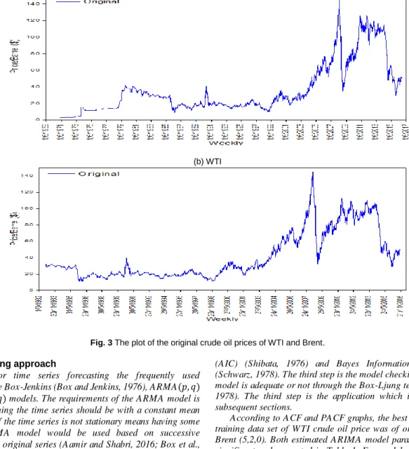
The basic purpose of this study is the reconstruction of IMFs obtained from EEMD. For a better understanding of IMFs a time series 𝑌𝑡 is created with additive noise from two different components called

stochastic and deterministic. Sine function was used with an angular frequency equivalent to 2𝜋 to create a deterministic component while the stochastic component created with random process 𝜀(𝜇, 𝛿)

following a standard normal distribution 𝑧(0,1). Hence, the noisy time series was obtained by summing both components i.e. 𝑌𝑡= 𝑆𝑖𝑛(2𝜋𝑡) +

𝜀(0,1). So, this time series is used to generate the data for simulations (Rios & De Mello, 2013). Figure 2 represented the deterministic and stochastic components and the noisy time series.

Fig. 2 (a) deterministic (2𝜋𝑡) , (b) Stochastic𝜀(0,1), components used to create the noisy time series 𝑌𝑡 (c) 𝑌𝑡= 𝑆𝑖𝑛(2𝜋𝑡) + 𝜀(0,1).

Evaluation criteria

To check the proposed model competency with the other models used in this study would be measured by using three different evaluation criteria defined as follows:

a) Mean Absolute Error (MAE)

𝑀𝐴𝐸 =1

𝑇∑ |𝑌𝑡− 𝑌̂𝑡| 𝑇

𝑡=1 (5)

b) Root Mean Square Error (RMSE)

𝑅𝑀𝑆𝐸 =1

𝑇√∑ (𝑌𝑡− 𝑌̂𝑡) 2 𝑇

𝑡=1 (6)

c) Mean Absolute Percentage Error (MAPE)

𝑀𝐴𝑃𝐸 = 1 𝑇∑ | 𝑌𝑡−𝑌̂𝑡 𝑌𝑡 | 𝑇 𝑡=1 × 100 (7)

where 𝑌𝑡 represents the original value at the given time 𝑡, 𝑇 used for a

total number of predictions and 𝑌̂𝑡 represented the forecasted value at

time 𝑡. The predicting model accuracy is one of the most important criteria when there are some other competing models. For the validation of the proposed method two weekly crude oil prices series are used.

DATA MATERIAL, MODEL DEVELOPMENT, RESULTS AND DISCUSSIONS

Overview of the data used in this study

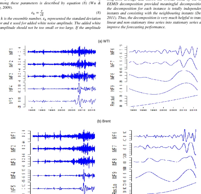
In this study, the two-well-known benchmark crude oil prices series are used for testing purpose i.e. WTI and Brent. The Brent data series comprising of 2440 weeks from February 01, 1970 to October 28, 2016,

0 200 400 600 800 1000 -1 .0 -0 .5 0. 0 0. 5 1. 0 Si ne W av e 0 200 400 600 800 1000 -2 -1 0 1 2 3 e( 0, 1) 0 200 400 600 800 1000 -3 -1 0 1 2 3 Y( t)

and WTI data series comprising of 1764 weeks from January 30, 1983, to October 28, 2016. The reason behind the selection of two different periods is to check the generalizability and robustness of the proposed procedure that the proposed procedure performs well and produce efficient results in two different periods as well as with a different number of forecasts. The sample data of both crude oil prices distributed in two different groups i.e. training and testing. The training

set consists of the first 80 per cent of the total observations while the last 20 per cent used as a testing set for model evaluation. Figure 3 representing the plots of both data sets. It is clear from figure 3 that there is no seasonal effect on either of data sets and reflects the two effects i.e. trend and random.

(a) Brent

(b) WTI

Fig. 3 The plot of the original crude oil prices of WTI and Brent. ARIMA modelling approach

Generally, for time series forecasting the frequently used

methodologies are Box-Jenkins (Box and Jenkins, 1976), ARMA(𝑝, 𝑞)

or ARIMA(𝑝, 𝑑, 𝑞) models. The requirements of the ARMA model is

stationarity, meaning the time series should be with a constant mean level. However, if the time series is not stationary means having some trend, the ARIMA model would be used based on successive differences of the original series (Aamir and Shabri, 2016; Box et al., 2015). To check stationarity Augmented Dickey-Fuller (ADF) (Elliott

et al., 1996) test is used. There are four main steps when using ARMA models: identification of the accurate model, estimation of parameters, model checking and application. The most important step is the identification of the model carrying in two steps: to achieve stationarity appropriate number of differencing of the series is performed if necessary and determination of appropriate order of AR and MA terms. For the best order of AR and MA terms (Box and Jenkins, 1976) used the ACF and PACF as a basic tool, which is the basic review of the graphs. However, other criteria are also used to select the best model through theoretical approaches i.e. Akaike’s Information Criterion

(AIC) (Shibata, 1976) and Bayes Information Criterion (BIC) (Schwarz, 1978). The third step is the model checking that the selected model is adequate or not through the Box-Ljung test (Ljung and Box, 1978). The third step is the application which is presented in the subsequent sections.

According to ACF and PACF graphs, the best ARIMA model for training data set of WTI crude oil price was of order (1,1,2) and for Brent (5,2,0). Both estimated ARIMA model parameters were highly significant and presented in Table 1. For model adequacy, the fitted model residuals were tested against the randomness, that the residuals are random or not. The p-values of the Box-Ljung test for both fitted models were (0.1094) and (0.1481) respectively. Which suggested that both model residuals distributed normally with 5% level of significance.

The forecasting accuracy of ARIMA models was measured using three descriptive methods discussed in the preceding sections. To reflect the fitted model forecasting accuracy 324 observations of WTI and 445 observations of Brent crude oil prices were used as testing data sets. All forecasting accuracy measures are presented in Table 8 for both crude oil prices.

Aamir et al. / Malaysian Journal of Fundamental and Applied Sciences Vol. 14, No. 4 (2018) 471-483 Table 1 Parameter estimation of ARIMA model for WTI and Brent series.

Decomposition of crude oil prices using EEMD

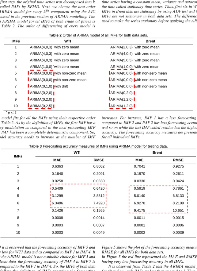
The two parameters being set in advance when using EEMD which directly affect the decomposition algorithm. These parameters are the number of ensemble and white noise amplitude. The already existing rule among these parameters is described by equation (8) (Wu & Huang, 2009).

𝜀𝑘= 𝑒

√𝑘 (8)

where 𝑘 is the ensemble number, 𝜀𝑘 represented the standard deviation

of error and 𝑒 used for added white noise amplitude. The added white noise amplitude should not be too small or too large. If the amplitude

is too small, then it may not change the extrema/minima of the EMD in a result produced the same IMFs as produced by EMD. On another side, if the amplitude is too large in result it produced some redundant IMFs. Wu and Huang (2009) suggested based on experimental observations that the amplitude of the added white noise is around 0.2 times of the sample standard deviation. Zhang et al., (2010) also investigated the parameter settings of the EEMD algorithm for different applications but their findings for adding white noise amplitude was not different than the (Wu and Huang, 2009). The EEMD strategy is employed in this study with the white noise amplitude of 0.2 times standard deviation and the ensemble number equal to 100. More details can be found about the ensemble number and amplitude of noise in the work of (Wu and Huang, 2009).

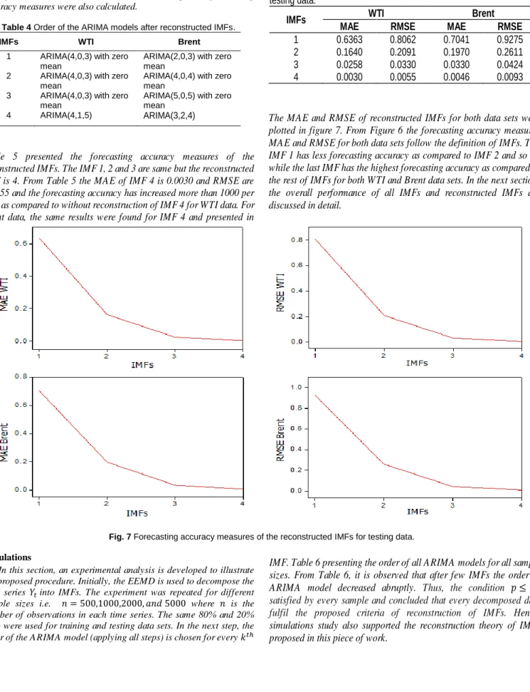
EEMD technique can be employed to both weekly crude oil prices time series using the above description. Both the crude oil prices series were decomposed into 9 IMFs and one residue. All IMFs and residue were independent, and their plots are shown in figure 4. From figure 4 (a) and (b) clears that IMF1, IMF2, and IMF3 have the highest frequency, maximum amplitude, and low wavelength. After the IMF3, the subsequent IMFs changing their frequencies and amplitude from maximum to minimum, wavelength from minimum to maximum. While the last component residue is a mode varying slowly around the long-term average and shows the overall trend of the time series. EEMD decomposition provided meaningful decomposition whereas the decomposition for each instance is totally independent of other instants and consisting with the neighbouring instants (Debert et al., 2011). Thus, the decomposition is very much helpful to transform non-linear and non-stationary time series into stationary series and used to improve the forecasting performance.

(a) WTI

(b) Brent

Fig. 4 IMFs and Residual plot of WTI and Brent series. Parameters Estimate t-value p-value

WTI (1,1,2) 𝜃1 0.8831 25.2845 < 0.0001 𝜇1 -0.9325 -21.2983 < 0.0001 𝜇2 0.0979 3.6186 0.00030 Brent (5,2,0) 𝜃1 -0.8493 -38.3817 < 0.0001 𝜃2 -0.6252 -21.9562 < 0.0001 𝜃3 -0.4593 -15.2652 < 0.0001 𝜃4 -0.3172 -11.0912 < 0.0001 𝜃5 -0.1705 -7.5852 < 0.0001

Reconstruction of IMFs

The proposed methodology in this study is the reconstruction of IMFs. In the first step, the original time series was decomposed into 𝑘 components called IMFs by EEMD. Next, we choose the best order (𝑝, 𝑑, 𝑞) of ARIMA model for every 𝑘𝑡ℎ _{component using the AIC}

criterion discussed in the previous section of ARIMA modelling. The order of each ARIMA model for all IMFs of both crude oil prices is presented in Table 2. The order of differencing of every model is

different in Table 2 because some of the series are stationary when a series a stationary then no need to take the difference of that series. A time series having a constant mean, variance and autocorrelation over the time called stationary time series. Thus, first six in WTI and seven IMFs in Brent data are stationary by using ADF test and the rest of the IMFs are not stationary in both data sets. The difference operator is used to make the series stationary before applying the ARIMA model.

Table 2 Order of ARIMA model of all IMFs for both data sets.

IMFs WTI Brent

1 ARIMA(4,0,3) with zero mean ARIMA(2,0,3) with zero mean 2 ARIMA(4,0,3) with zero mean ARIMA(4,0,4) with zero mean 3 ARIMA(4,0,3) with zero mean ARIMA(5,0,5) with zero mean 4 ARIMA(1,0,0) *_{with zero mean ARIMA(1,0,0)} *_{with zero mean} 5 ARIMA(0,0,0) with non-zero mean ARIMA(0,0,0) with non-zero mean 6 ARIMA(0,0,0) with non-zero mean ARIMA(0,0,0) with non-zero mean 7 ARIMA(0,1,0) with drift ARIMA(0,0,0) with non-zero mean

8 ARIMA(0,2,0) ARIMA(0,2,0)

9 ARIMA(0,2,0) ARIMA(1,2,0)

10 ARIMA(0,2,5) ARIMA(1,2,0)

* _{𝑝 ≤ 1}

The ARIMA model fits for all the IMFs using their respective order mentioned in Table 2. As by the definition of IMFs, the first IMF has a high-frequency modulation as compared to the next proceeding IMF while the last IMF has been a completely deterministic component. So, the fitted model accuracy needs to increase as the number of IMF

increases. For instance, IMF 1 has a less forecasting accuracy as compared to IMF 2 and IMF 2 has less forecasting accuracy as IMF 3 and so on while the last IMF called residue has the highest forecasting accuracy. The forecasting accuracy measures are presented in Table 3 for all individual IMFs.

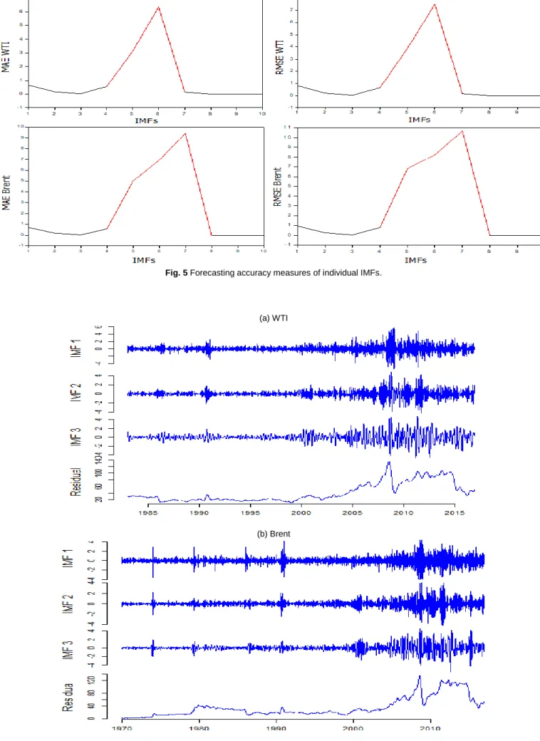
Table 3 Forecasting accuracy measures of IMFs using ARIMA model for testing data. IMFs

WTI Brent

MAE RMSE MAE RMSE

1 0.6363 0.8062 0.7041 0.9275 2 0.1640 0.2091 0.1970 0.2611 3 0.0258 0.0330 0.0330 0.0424 4 0.5409 0.6420 0.5919 0.7861 5 3.1299 3.8812 5.0140 6.8133 6 6.3486 7.4920 6.9270 8.2109 7 0.1426 0.1565 9.4175 10.651 8 0.0008 0.0014 0.0011 0.0015 9 0.0003 0.0007 0.0001 0.0006 10 0.0003 0.0049 0.0002 0.0039

From Table 3 it is observed that the forecasting accuracy of IMF 5 and IMF 6 is very low for WTI data and as compared to IMF 1 to IMF 4. It indicates that the ARIMA model is not a suitable choice for IMF 5 and IMF 6. For Brent data, the forecasting accuracy of IMF 4 to IMF 7 is very low as compared to the IMF 1 to IMF 4. So, the IMFs of both data sets did not follow the definition of IMFs regarding the forecasting accuracy of the models. The definition of IMFs is that the IMF 1 has more stochastic as compared to IMF 2 while the last IMF should be more deterministic as compared to the second last IMF and so on.

Figure 5 shows the plot of the forecasting accuracy measures MAE and RMSE for all IMFs for both data sets.

In Figure 5 the red line represented the MAE and RMSE of the IMFs having very low forecasting accuracy in all IMFs.

It is observed from Table 2 that the ARIMA model parameters 𝑝 for 4th _{and onwards IMFs are less than or equal to 1. Thus, the condition}

𝑝 ≤ 1is satisfied by 4th _{to 10}th _{IMF. So according to the proposed rule,}

all these IMFs be combined for further analysis. Thus, the total number of IMFs to be used for further analysis is 4 and plotted in Figure 6 for

Aamir et al. / Malaysian Journal of Fundamental and Applied Sciences Vol. 14, No. 4 (2018) 471-483

Fig. 5 Forecasting accuracy measures of individual IMFs.

(a) WTI

(b) Brent

Using the information in Table 4 the respective ARIMA model were fitted for both WTI and Brent IMFs and their respective forecasting accuracy measures were also calculated.

Table 4 Order of the ARIMA models after reconstructed IMFs.

IMFs WTI Brent

1 ARIMA(4,0,3) with zero mean

ARIMA(2,0,3) with zero mean

2 ARIMA(4,0,3) with zero mean

ARIMA(4,0,4) with zero mean

3 ARIMA(4,0,3) with zero mean

ARIMA(5,0,5) with zero mean

4 ARIMA(4,1,5) ARIMA(3,2,4)

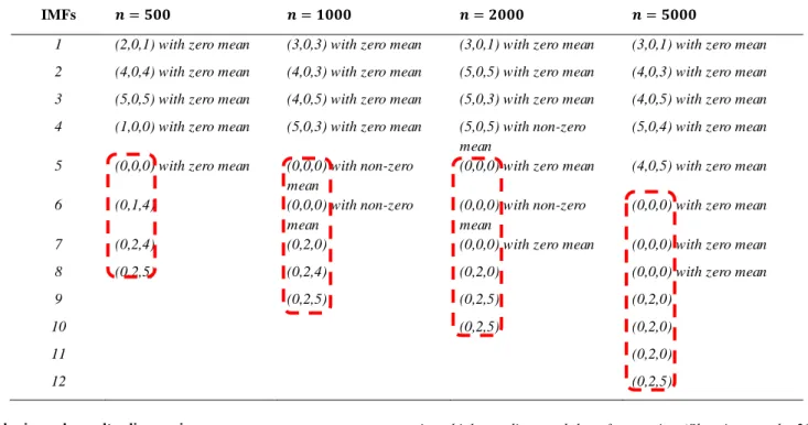
Table 5 presented the forecasting accuracy measures of the reconstructed IMFs. The IMF 1, 2 and 3 are same but the reconstructed IMF is 4. From Table 5 the MAE of IMF 4 is 0.0030 and RMSE are 0.0055 and the forecasting accuracy has increased more than 1000 per cent as compared to without reconstruction of IMF 4 for WTI data. For Brent data, the same results were found for IMF 4 and presented in Table 5.

Table 5

Forecasting accuracy measures of the reconstructed IMFs for

testing data

.

IMFs

WTI

Brent

MAE

RMSE

MAE

RMSE

1

0.6363

0.8062

0.7041

0.9275

2

0.1640

0.2091

0.1970

0.2611

3

0.0258

0.0330

0.0330

0.0424

4

0.0030

0.0055

0.0046

0.0093

The MAE and RMSE of reconstructed IMFs for both data sets were

plotted in figure 7. From Figure 6 the forecasting accuracy measures

MAE and RMSE for both data sets follow the definition of IMFs. The

IMF 1 has less forecasting accuracy as compared to IMF 2 and so on

while the last IMF has the highest forecasting accuracy as compared to

the rest of IMFs for both WTI and Brent data sets. In the next section,

the overall performance of all IMFs and reconstructed IMFs are

discussed in detail.

Fig. 7 Forecasting accuracy measures of the reconstructed IMFs for testing data. Simulations

In this section, an experimental analysis is developed to illustrate the proposed procedure. Initially, the EEMD is used to decompose the time series 𝑌𝑡into IMFs. The experiment was repeated for different

sample sizes i.e. 𝑛 = 500,1000,2000, 𝑎𝑛𝑑 5000 where 𝑛 is the number of observations in each time series. The same 80% and 20% ratio were used for training and testing data sets. In the next step, the order of the ARIMA model (applying all steps) is chosen for every 𝑘𝑡ℎ

IMF. Table 6 presenting the order of all ARIMA models for all sample

sizes. From Table 6, it is observed that after few IMFs the order of

ARIMA model decreased abruptly.

Thus, the condition

𝑝 ≤ 1

is

satisfied by every sample and concluded that every decomposed data

fulfil the proposed criteria of reconstruction of IMFs. H

ence,

simulations study also supported the reconstruction theory of IMFs

proposed in this piece of work.

Aamir et al. / Malaysian Journal of Fundamental and Applied Sciences Vol. 14, No. 4 (2018) 471-483 Table 6 Order of ARIMA (𝑝, 𝑑, 𝑞) model for 𝑌𝑡= 𝑆𝑖𝑛(2𝜋𝑡) + 𝜀(0,1).

IMFs 𝒏 = 𝟓𝟎𝟎 𝒏 = 𝟏𝟎𝟎𝟎 𝒏 = 𝟐𝟎𝟎𝟎 𝒏 = 𝟓𝟎𝟎𝟎

1 (2,0,1) with zero mean (3,0,3) with zero mean (3,0,1) with zero mean (3,0,1) with zero mean 2 (4,0,4) with zero mean (4,0,3) with zero mean (5,0,5) with zero mean (4,0,3) with zero mean 3 (5,0,5) with zero mean (4,0,5) with zero mean (5,0,3) with zero mean (4,0,5) with zero mean 4 (1,0,0) with zero mean (5,0,3) with zero mean (5,0,5) with non-zero

mean

(5,0,4) with zero mean 5 (0,0,0) with zero mean (0,0,0) with non-zero

mean

(0,0,0) with zero mean (4,0,5) with zero mean

6 (0,1,4) (0,0,0) with non-zero

mean

(0,0,0) with non-zero mean

(0,0,0) with zero mean

7 (0,2,4) (0,2,0) (0,0,0) with zero mean (0,0,0) with zero mean

8 (0,2,5) (0,2,4) (0,2,0) (0,0,0) with zero mean

9 (0,2,5) (0,2,5) (0,2,0)

10 (0,2,5) (0,2,0)

11 (0,2,0)

12 (0,2,5)

Analysis and results discussions

In this section, the overall results of all models are discussed in detail. The three descriptive measures MAE, RMSE, and MAPE were used for validation of the performance of the models. The six models were fitted for both data sets namely, individual ARIMA, EEMD-ARIMA (without reconstruction of IMFs), EEMD-SD-EEMD-ARIMA (with reconstruction of IMFs into stochastic and deterministic (Rios and De Mello, 2013)), EEMD-HML-ARIMA (with reconstruction of IMFs

into high, medium and low frequencies (Shu-ping et al., 2014)), EEMD-FC-ARIMA (with reconstruction of IMFs from fine to coarse (Yan et al., 2014)) and the last is the proposed method EEMD-PQ-ARIMA (with reconstruction of IMFs based on order of Autoregressive term). Table 7 presenting the number of reconstructed IMFs based on different procedures and the same used for forecasting of both crude oil prices.

Table 7 Reconstruction of IMFs based on different methods.

DATA Model IMF-1 IMF-2 IMF-3 IMF-4

Brent EEMD-PQ-ARIMA 1 2 3 4 – 10 EEMD-FC-ARIMA 1 – 5 6 – 9 10 EEMD-HML-ARIMA 1 – 3 4 – 8 9 – 10 EEMD-SD-ARIMA 1 – 5 5 – 10 WTI EEMD-PQ-ARIMA 1 2 3 4 – 10 EEMD-FC-ARIMA 1 – 4 5 – 9 10 EEMD-HML-ARIMA 1 – 3 4 – 7 8 – 10 EEMD-SD-ARIMA 1 – 4 5 – 10

The fitted model's accuracy is presenting in Table 8. From Table 8 it is observed that the performance of the model EEMD-ARIMA was worst as compared to the individual ARIMA, SD-ARIMA, EEMD-HML-ARIMA, EEMD-FC-ARIMA and EEMD-PQ-ARIMA model. The reason behind that poor performance is the misuse of the ARIMA model for the IMFs stated in Table 3 highlighted with the red dotted line because for all IMFs the ARIMA model is not suitable. The forecasting accuracy of all the reconstruction of IMFs procedure increased as compared to the single ARIMA model. In the

reconstruction of IMFs methods, the performance of the EEMD-SD-ARIMA and EEMD-FC-EEMD-SD-ARIMA models are almost the same but not better than the EEMD-HML-ARIMA model. Next is the performance evaluation of the proposed EEMD-PQ-ARIMA model. The forecasting accuracy of the EEMD-PQ-ARIMA model increased significantly and outperform all the other reconstruction of IMFs technique. The forecasting accuracy of the proposed EEMD-PQ-ARIMA model has been increased more than 100 per cent for all accuracy measures for both crude oil prices.

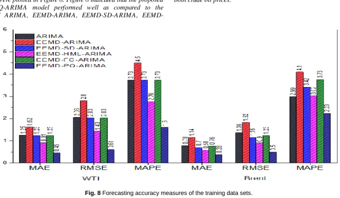
Table 8 Fitted model accuracy measurements for training datasets. Model

WTI Brent

MAE RMSE MAPE MAE RMSE MAPE

ARIMA 1.25 2.06 3.73 0.78 1.36 2.99 EEMD-ARIMA 1.62 2.80 4.50 1.14 1.82 4.10 EEMD-SD-ARIMA 1.23 2.03 3.73 0.70 1.16 3.42 EEMD-HML-ARIMA 0.91 1.43 2.76 0.58 0.90 3.02 EEMD-FC-ARIMA 1.23 2.03 3.73 0.76 1.23 3.76 EEMD-PQ-ARIMA 0.45 0.61 1.60 0.38 0.50 2.23

The forecasting accuracy measures for all the six fitted models for both data sets were plotted in Figure 8. Figure 8 indicated that the proposed EEMD-PQ-ARIMA model performed well as compared to the individual ARIMA, ARIMA, SD-ARIMA,

EEMD-HML-ARIMA and EEMD-FC-ARIMA model for training data sets of both crude oil prices.

Fig. 8 Forecasting accuracy measures of the training data sets.

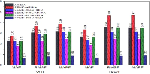
The next is the most important comparison of the six competing models with respect to the forecasting accuracy for testing data sets. Table 9 presenting the forecasting accuracy of all models for WTI and Brent data. From Table 9 it is observed that the forecasting accuracy of the EEMD-ARIMA model was very low as compared to the ARIMA, EEMD-SD-ARIMA, EEMD-HML-ARIMA and EEMD-FC-ARIMA and EEMD-PQ-ARIMA model for all three descriptive measures. As

compared to the ARIMA, EEMD-ARIMA, EEMD-SD-ARIMA,

EEMD-HML-ARIMA and EEMD-FC-ARIMA models the

performance of the EEMD-PQ-ARIMA model has improved more than two hundred per cent for all the evaluation measures. Which shows that the proposed model improves the forecasting accuracy of both data sets significantly.

Table 9 Forecasting accuracy measurements for testing data sets.

Model WTI Brent

MAE RMSE MAPE MAE RMSE MAPE

ARIMA 2.30 3.07 3.18 2.68 3.59 3.53 EEMD-ARIMA 2.76 3.69 3.89 3.34 4.68 4.70 EEMD-SD-ARIMA 2.25 2.94 3.14 2.37 3.14 3.15 EEMD-HML-ARIMA 1.80 2.29 2.47 1.90 2.47 2.47 EEMD-FC-ARIMA 2.26 2.95 3.15 2.64 3.53 3.49 EEMD-PQ-ARIMA 0.65 0.81 0.89 0.69 0.88 0.92

Aamir et al. / Malaysian Journal of Fundamental and Applied Sciences Vol. 14, No. 4 (2018) 471-483

Fig. 9 Forecasting accuracy measures of testing data sets.

Subsequently, the comparison of the forecasted values of the testing data sets of ARIMA and proposed model EEMD-PQ-ARIMA with the original data are presenting in Figure 10 for both data sets. Figure 10 (a) presenting the WTI data and exhibited biannually on the plot. From the figure, the EEMD-PQ-ARIMA model forecasted values are very much close to the original data and adjust quickly to follow the pattern of the data, next is the ARIMA model whose graph also showed some good forecasts but it values not adjusted that much quicker as compared to EEMD-PQ-ARIMA model to follow the pattern. For a clearer picture, the last 6 months original and forecasted values were more focused and present in the new graph. In the new graph, the last 6 months data exhibited on two weekly bases. The new graph showed a clearer picture of the fitted model forecasted values with the original testing series of WTI. It is observed from the new graph that the proposed model EEMD-PQ-ARIMA forecasted values were closer to the original data and moving in the same direction of the original series.

In other words, the proposed model has the ability of quick recovery of the pattern of the data and adjust the values and produce a more accurate forecast for the future as compared to single ARIMA model.

Figure 10 (b) presenting the Brent crude oil price original testing series and the forecasted values of the fitted models. From the figure, it is observed that the proposed EEMD-PQ-ARIMA model forecasted values are very much close to original data. The weekly original data was exhibited bi-annually on the graph. For the clearer relationship between the original data and the forecasted values of all the models the last 10 months data were more focused and plotted in the new graph distinguishing it with a different colour. In the new graph, the relationship is clearer, and the data exhibited on three weekly bases. The forecasted values of the proposed EEMD-PQ-ARIMA model are closer to the original data as compared to the ARIMA model. Thus, figure 10 (a) and (b) showed that the proposed model EEMD-PQ-ARIMA performed well and produced more accurate forecasts for the future.

(a) WTI

(b) Brent

CONCLUSION

A new method of reconstruction of IMFs was proposed in this study to improve the forecasting accuracy of the crude oil prices. Two different crude oil prices datasets were used to check the performance of the proposed procedure. The empirical results showed that the decomposition ensemble methodology was effective. However, the MAE, RMSE and MAPE results indicated that the reconstruction of IMFs was the more effective approach for improving the forecasting accuracy of crude oil prices based on order of the ARIMA model. There are several advantages of the proposed approach: Firstly, the essential rule of the EEMD is extremely straightforward which can give a better understanding of the inner factors in crude oil prices. Secondly, the reconstruction of IMFs avoids the problem of non-zero mean in IMFs which is helpful to carry out ARIMA modelling. Thirdly, ARIMA prediction requires just data of the crude oil prices being referred to. Fourthly, the proposed model needs less computational time. Finally, the proposed EEMD-PQ-ARIMA model does not require complex decision-making about the unequivocal form of models for each case. In this way, building up a reconstructed mixture model may prompt more precise and stable estimating comes about, and might be useful for determining the crude oil prices time series for an extensive variety of issues identified with the successful value administration.

In addition to crude oil price data, the proposed methodology should be applied to a more complex task of forecasting to test its generalizability and robustness and especially to nonlinear data. Furthermore, based on the reconstruction of the IMFs idea, other more powerful decomposition ensemble models should be developed accordingly, for individual model prediction as well as for ensemble model predictions. An attempt will be carried out soon.

REFERENCES

Aamir, M., Shabri, A. (2016). Modelling and forecasting monthly crude oil price of Pakistan: A comparative study of ARIMA, GARCH and ARIMA Kalman

model. Paper presented at the Advances in Industrial and Applied

Mathematics: Proceedings of 23rd Malaysian National Symposium of Mathematical Sciences (SKSM23). 24-26 November. Johor Bahru: AIP Publishing.

Aamir, M., Shabri, A. (2018). improving crude oil price forecasting accuracy via decomposition and ensemble model by reconstructing the stochastic and

deterministic influences. Advanced Science Letters, 24(6), 4337- 4342.

Box, G. E., Jenkins, G. M. (1976). Time Series Analysis: Forecasting and Control, revised ed. San Francisco: Holden-Day.

Box, G. E., Jenkins, G. M., Reinsel, G. C., Ljung, G. M. (2015). Time Series Analysis: Forecasting and Control. Hoboken: John Wiley Sons.

Chiroma, H., Abdulkareem, S., Herawan, T. (2015). Evolutionary neural network model for West Texas intermediate crude oil price prediction.

Applied Energy, 142, 266-273.

Debert, S., Pachebat, M., Valeau, V., Gervais, Y. (2011).

Ensemble-empirical-mode-decomposition method for instantaneous spatial-multi-scale

decomposition of wall-pressure fluctuations under a turbulent flow.

Experiments in Fluids, 50(2), 339-350.

Elliott, G., Rothenberg, T. J., Stock, J. H. (1996). Efficient tests for an

autoregressive unit root. Econometrica, 64(4), 813-836.

Flandrin, P., Goncalves, P. (2004). Empirical mode decompositions as

data-driven wavelet-like expansions. International Journal of Wavelets,

Multiresolution and Information Processing, 2(04), 477-496.

Flandrin, P., Rilling, G., Goncalves, P. (2004). Empirical mode decomposition as a filter bank. IEEE Signal Processing Letters, 11(2), 112-114. Huang, N. E., Shen, Z., Long, S. R. (1999). A new view of nonlinear water

waves: The Hilbert Spectrum 1. Annual Review Of Fluid Mechanics, 31(1),

417-457.

Khashman, A., Nwulu, N. I. (2011). Intelligent prediction of crude oil price

using support vector machines. Paper presented at the IEEE 9th

International Symposium on Applied Machine Intelligence and Informatics

Liu, H., Tian, H.-q., Pan, D.-f., Li, Y.-f. (2013). Forecasting models for wind speed using wavelet, wavelet packet, time series and Artificial Neural

Networks. Applied Energy, 107, 191-208.

Ljung, G. M., Box, G. E. (1978). On a measure of lack of fit in time series models. Biometrika, 65(2), 297-303.

Mirmirani, S., Cheng Li, H. (2004). A comparison of VAR and neural networks with genetic algorithm in forecasting price of oil Applications of Artificial Intelligence in Finance and Economics (pp. 203-223): Emerald Group Publishing Limited.

Montgomery, D. C., Jennings, C. L., Kulahci, M. (2015). Introduction to Time

Series Analysis and Forecasting: John Wiley Sons.

Movagharnejad, K., Mehdizadeh, B., Banihashemi, M., Kordkheili, M. S. (2011). Forecasting the differences between various commercial oil prices

in the Persian Gulf region by neural network. Energy, 36(7), 3979-3984.

Nomikos, N., Andriosopoulos, K. (2012). Modelling energy spot prices:

Empirical evidence from NYMEX. Energy Economics, 34(4), 1153-1169.

Rios, R. A., De Mello, R. F. (2013). Improving time series modeling by

decomposing and analyzing stochastic and deterministic influences. Signal

Processing, 93(11), 3001-3013.

Schwarz, G. (1978). Estimating the dimension of a model. The Annals of

Statistics, 6(2), 461-464.

Shibata, R. (1976). Selection of the order of an autoregressive model by Akaike's information criterion. Biometrika, 117-126.

Shu-ping, W., Ai-mei, H., Zhen-xin, W., Ya-qing, L., Xiao-wei, B. (2014). Multiscale combined model based on run-length-judgment method and its

application in oil price forecasting. Mathematical Problems in Engineering,

2014, 1-9.

Tang, L., Dai, W., Yu, L., Wang, S. (2015). A novel CEEMD-based EELM ensemble learning paradigm for crude oil price forecasting. International Journal of Information Technology Decision Making, 14(01), 141-169. Tang, L., Yu, L., Wang, S., Li, J., Wang, S. (2012). A novel hybrid ensemble

learning paradigm for nuclear energy consumption forecasting. Applied

Energy, 93, 432-443.

Valipour, M., Banihabib, M. E., Behbahani, S. M. R. (2013). Comparison of the ARMA, ARIMA, and the autoregressive artificial neural network models in

forecasting the monthly inflow of Dez dam reservoir. Journal of Hydrology,

476, 433-441.

Wang, S. Y., L.A. Yu and K.K. Lai,. (2005). Crude oil price forecasting with

TEI@ I methodology. Journal of Systems Science and Complexity, 18(2),

145-166.

Wang, W.-c., Chau, K.-w., Xu, D.-m., Chen, X.-Y. (2015). Improving forecasting accuracy of annual runoff time series using ARIMA based on

EEMD decomposition. Water Resources Management, 29(8), 2655-2675.

Wu, Z., Feng, J., Qiao, F., Tan, Z.-M. (2016). Fast multidimensional ensemble empirical mode decomposition for the analysis of big spatio-temporal datasets. Philosophical Transactions of the Royal Society A, 374(2065), 20150197.

Wu, Z., Huang, N. E. (2004). A study of the characteristics of white noise using

the empirical mode decomposition method. Proceedings of the Royal

Society of London A: Mathematical, Physical and Engineering Sciences.

Wu, Z., Huang, N. E. (2009). Ensemble empirical mode decomposition: a

noise-assisted data analysis method. Advances in Adaptive Data Analysis, 1(01),

1-41.

Wu, Z., Huang, N. E. (2010). On the filtering properties of the empirical mode

decomposition. Advances in Adaptive Data Analysis, 2(04), 397-414.

Xiang, Y., Zhuang, X. H. (2013). Application of ARIMA model in short-term prediction of international crude oil price.Advanced Materials Research, 798-799, 979-982.

Xie, W., Yu, L., Xu, S., Wang, S. (2006). A new method for crude oil price

forecasting based on support vector machines Computational Science–ICCS

2006 (pp. 444-451): Springer.

Yan, Q., Wang, S., Li, B. (2014). Forecasting uranium resource price prediction by extreme learning machine with empirical mode decomposition and phase

space reconstruction. Discrete Dynamics in Nature and Society, 2014, 1-10.

Yu, L., Dai, W., Tang, L. (2016). A novel decomposition ensemble model with extended extreme learning machine for crude oil price forecasting.

Engineering Applications of Artificial Intelligence, 47, 110-121. Yu, L., Wang, S., Lai, K. K. (2008). Forecasting crude oil price with an

EMD-based neural network ensemble learning paradigm. Energy Economics,