Crude oil price forecasting based on hybridizing wavelet multiple linear regression model, particle swarm optimization techniques, and principal component analysis

(1)

Research Article

Crude Oil Price Forecasting Based on Hybridizing Wavelet

Multiple Linear Regression Model, Particle Swarm Optimization

Techniques, and Principal Component Analysis

Ani Shabri

1

and Ruhaidah Samsudin

2

1_{Department of Science Mathematic, Faculty of Science, Universiti Teknologi Malaysia, 81310 Johor, Malaysia}

2_{Department of Software Engineering, Faculty of Computing, Universiti Teknologi Malaysia (UTM), 81310 Johor, Malaysia} Correspondence should be addressed to Ani Shabri; ani [email protected]

Received 31 December 2013; Accepted 18 March 2014; Published 8 May 2014 Academic Editors: S. Balochian, V. Bhatnagar, and Y. Zhang

Copyright © 2014 A. Shabri and R. Samsudin. This is an open access article distributed under the Creative Commons Attribution License, which permits unrestricted use, distribution, and reproduction in any medium, provided the original work is properly cited.

Crude oil prices do play significant role in the global economy and are a key input into option pricing formulas, portfolio allocation, and risk measurement. In this paper, a hybrid model integrating wavelet and multiple linear regressions (MLR) is proposed for crude oil price forecasting. In this model, Mallat wavelet transform is first selected to decompose an original time series into several subseries with different scale. Then, the principal component analysis (PCA) is used in processing subseries data in MLR for crude oil price forecasting. The particle swarm optimization (PSO) is used to adopt the optimal parameters of the MLR model. To assess the effectiveness of this model, daily crude oil market, West Texas Intermediate (WTI), has been used as the case study. Time series prediction capability performance of the WMLR model is compared with the MLR, ARIMA, and GARCH models using various statistics measures. The experimental results show that the proposed model outperforms the individual models in forecasting of the crude oil prices series.

1. Introduction

Crude oil prices do play significant role in the global economy and constitute an important factor affecting government’s plans and commercial sectors. Forecasting crude oil price is among the most important issues facing energy economists. Therefore, proactive knowledge of its future fluctuations can lead to better decisions in several managerial levels.

The literature dealing with forecasting crude oil is sub-stantial. The application of the classical time series models

such as autoregressive moving average (ARMA) (Yu et al. [1],

Mohammadi and Su [2], and Ahmad [3]) and econometric

model such as generalized autoregressive conditional

het-eroscedasticity (GARCH) type models (Agnolucci [4], Wei et

al. [5], Liu and Wan [6]) for crude oil forecasting has received

much attention in the last decade. But because the crude oil price has the volatility, nonlinearity, and irregularity, the classical and econometric model can lead to the decrease of the accuracy.

Due to the limitations of the classical and econometric models, soft-computing models, such as neural fuzzy

(Ghaf-fari and Zare [7]), artificial neural networks (Kaboudan [8],

Mirmirani and Li [9], Shambora and Rossiter [10], and Yu et

al. [11]), support vector machines (Xie et al. [12]), and genetic

programming (GP), provide powerful solutions to nonlinear crude oil price prediction. Many experiments found that the soft-computing models often had some advantages over statistical-based models. However, these AI models also have their own shortcomings and disadvantages. For example, ANN often suffers from local minima and over-fitting, while other soft-computing models, such as SVM and GP, including

ANN, are sensitive to parameter selection [1].

To remedy the above shortcomings, some hybrid meth-ods have been used recently to predict crude oil price and obtain the best performances. In last year, wavelet transform has become a useful method for analyzing such as variations, periodicities, and trends in time series. The hybrid models with wavelet transform processes have been improved for

Volume 2014, Article ID 854520, 8 pages http://dx.doi.org/10.1155/2014/854520

(2)

forecasting. For example wavelet-neural network (Jammazi

and Aloui [13], Qunli et al. [14], and Yousefi et al. [15]),

wavelet-least square support vector machines (LSVM) (Bao

et al. [16]), and wavelet-fuzzy neural network (Liu et al. [17])

have been employed recently on some studies in crude oil forecasting. They observed that the wavelet transform fairly improves forecasting accuracy.

A major drawback of wavelet transform for direction prediction is that the input variables lie in a high-dimensional feature space depends on the number of sub-time series components. Because the number of sub-time series compo-nents for wavelet is inadvisable to be too many, in this study principal component analysis (PCA) is proposed to reduce the dimensions of sub-time series components.

The multiple linear regressions (MLR) model that is much easier to interpret is considered as an alternative to ANN model. In this paper, a hybrid wavelet multiple linear regression (WMLR) model integrating wavelet and MLR is proposed for short-term daily crude oil price forecasting. The study applies particle swarm optimization (PSO) to adopt the optimal parameters to construct the MLR model. For verification purpose, the West Texas Intermediate (WTI) crude oil sport price is used to test the effectiveness of the proposed WMLR ensemble learning methodology. Finally to evaluate the model ability, the proposed model was compared with individual ARIMA and GARCH models.

2. Methodology

2.1. The ARIMA Model. The most comprehensive of all popu-lar and widely known statistical methods used for time series

forecasting are Box-Jenkins models (Box and Jenkins [18]).

It has achieved great success in both academic research and industrial applications during the last three decades. The general form of ARIMA models can be expressed as

𝑦_𝑡=∑𝑝

𝑖=1

𝜙_𝑖𝑦_𝑡−𝑖+∑𝑞

𝑖=1

𝜃_𝑖𝑒_𝑡−𝑖+ 𝑒_𝑡, (1)

where𝑝is the order of the autoregressive,𝑞is the order of the

moving average, and𝑒_𝑡is the random error. The Box-Jenkins

methodology is basically divided into four steps: identifica-tion, estimaidentifica-tion, diagnostic checking, and forecasting.

2.2. The GARCH Model. GARCH models have found exten-sive application in the literature and the most popular

volatil-ity model is GARCH (1, 1) model proposed by Bollerslev [19].

The standard GARCH (1, 1) can be described as follows:

𝑟_𝑡= 𝜇_𝑡+ 𝜀_𝑡= 𝜇_𝑡+ ℎ1/2_𝑡 𝜂_𝑡 𝜂_𝑡∼ 𝑁 (0, 1) ,

ℎ_𝑡= 𝜔 + 𝛼𝜀2_𝑡−1+ 𝛽ℎ_𝑡−1, (2)

where 𝜇_𝑡 denote the conditional mean andℎ_𝑡 is the

con-ditional variances and𝜂_𝑡 is a standardized error and 𝑟_𝑡 =

ln(𝑥_𝑡/𝑥_𝑡−1)is log return.

2.3. Multiple Linear Regressions. Multiple linear regressions (MLR) model is one of the modelling techniques to investi-gate the relationship between a dependent variable and

sev-eral independent variables. Let the MLR have𝑝independent

variables with𝑛observations. Thus the MLR can be written

as

𝑌 = 𝑤₀+ 𝑤₁𝑥_𝑖+ 𝑤₂𝑥₂+ ⋅ ⋅ ⋅ + 𝑤_𝑝𝑥_𝑝+ 𝜀_𝑡, (3)

where𝑤are regression coefficients,𝑌is dependent variable,

𝑥_𝑖 are independent varaiables and 𝜀_𝑡 is fitting errors. The

method of least squares is generally used to estimate the coefficients model. In many applications, the results of a least squares fit are often unacceptable when the model is wrong or

when the model is misspecified (Bozdogan and Howe [20]).

In this study, particle swarm optimization (PSO) method is presented to determine the optimal parameters of the MLR model. The PSO methods have proven to be very effective in solving a variety of difficult global optimization problems

in forecasting (Chen and Kao [21] and Alwee et al. [22]),

heat problem (Ma et al. [23] and Tyagi and Pandit [24]), and

dynamic environments (Liu et al. [25]).

The classic solution of MLR model involves the mini-mization of the sum of the square errors between the model-predicted value and the corresponding data value:

min𝑓 (𝑤) =

𝑛

∑

𝑖=1

(𝑌_𝑖− ̂𝑌_𝑖)2, (4)

where 𝑛is the number of training data samples, 𝑌_𝑖 is the

actual value, and ̂𝑌_𝑖 is the forecasted value of train data.

The same methodology was used to solve this problem using

PSO algorithms. The solution with a smaller fitness𝑓(𝑤)of

the training data set has a better chance of surviving in the successive generations.

2.4. Particle Swarm Optimization. Particle swarm optimiza-tion (PSO) is a populaoptimiza-tion-based heuristic method inspired by the collective motion of biological organisms, such as bird flocking and fish schooling, to simulate the seeking

behavior to a food source (Bratton and Kennedy [26]). The

population of PSO is called a swarm and each individual in the population of PSO is called a particle. The PSO begins with a random population and searchers for fitness optimum just like genetic algorithm (GA). To find the optimum solution, each particle adjusts the direction through the best

experience which it has found (𝑝best) and the best experience

that has been found by all other members (𝑔best). Therefore,

the particles fly around in a multidimensional space towards the better area over the search process.

Each particle consists of three vectors: the position

for 𝑖th individual particle can be denoted as 𝑋_𝑖 =

(𝑥(1)

𝑖 , 𝑥(2)𝑖 , . . . , 𝑥(𝐷)𝑖 ), the best previous position𝑝bestthat the

𝑖th particle has searched is 𝑃_𝑖 = (𝑝(1)_𝑖 , 𝑝(2)_𝑖 , . . . , 𝑝(𝐷)_𝑖 ), and

the fly velocity of the 𝑖th is 𝑉_𝑖 = (V(1)_𝑖 ,V(2)_𝑖 , . . . ,V(𝐷)_𝑖 ). The

(3)

function varying from problem in hand. During the iterative

procedure, the𝑖th particle at iteration𝑡is updated by

V𝑑_𝑖 (𝑡 + 1) = 𝜔󸀠×V𝑑_𝑖 (𝑡) + 𝑐1× 𝜑1× [𝑝𝑖𝑑(𝑡) − 𝑥𝑑𝑖 (𝑡)]

+ 𝑐₂× 𝜑₂× [𝑝𝑑_𝑔(𝑡) − 𝑥𝑑_𝑖 (𝑡)] , 𝑥_𝑖𝑑(𝑡 + 1) = 𝑥𝑑_𝑖 (𝑡) +V𝑑_𝑖 (𝑡 + 1) ,

(5)

where𝜔is called inertia weight,𝑐₁and𝑐₂are acceleration

con-stants, and𝜑₁and𝜑₂are stochastic value of[0, 1]. In a PSO

system, particles change their positions at each time step until a relatively unchanging position has been encountered or a maximum number of iterations have been met. In general, the performance of each particle is measured according to a fitness function, which is problem dependent. In MLR model,

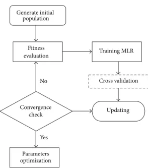
(4) is the fitness function under consideration.Figure 1shows

the flowchart of the developed PSO algorithm. For further details regarding PSO, please refer to Kennedy and Eberhart

[27] and Bratton and Kennedy [26].

2.5. Wavelet Analysis. Wavelet transformations provide ful decomposition of original time series by capturing use-ful information on various decomposition levels. Discrete wavelet transformation (DWT) is preferred in most of the forecasting problems because of its simplicity and ability to compute with less time. The DWT can be defined as

𝜓_𝑚,𝑛(𝑡 − 𝜏 𝑠 ) = 1 √𝑠𝑚/2 0 𝜓 (𝑡 − 𝑛𝜏0𝑠𝑚0 𝑠𝑚 0 ) , (6)

where𝑚and𝑛are integers that control the scale and time. The

most common choices for the parameters𝑠₀= 2and𝜏₀ = 1.

𝜓(𝑡)called the mother wavelet can be defined as∫_−∞∞ 𝜓(𝑡)𝑑𝑡 =

0.

For a discrete time series𝑥(𝑡)where𝑥(𝑡)occurs at discrete

time𝑡, the DWT becomes

𝑊_𝑚,𝑛= 2−𝑚/2𝑁−1∑

𝑡=0

𝜓 (2−𝑚𝑡 − 𝑛) 𝑥 (𝑡) , (7)

where𝑊_𝑚,𝑛is the wavelet coefficient for the discrete wavelet

at scale𝑠 = 2𝑚and𝜏 = 2𝑚𝑛. According to Mallat’s theory,

the original discrete time series𝑥(𝑡)can be decomposed into

a series of linearity independent approximation and detail signals by using the inverse DWT. The inverse DWT is given

by (Mallat [28]) 𝑥 (𝑡) = 𝑇 + ∑𝑀 𝑚=1 2𝑀−𝑚−1 ∑ 𝑡=0 𝑊𝑚,𝑛2 −𝑚/2_{𝜓 (2}−𝑚_{𝑡 − 𝑛)} ₍₈₎ or in a simple format as 𝑥 (𝑡) = 𝐴𝑀(𝑡) + 𝑀 ∑ 𝑚=1 𝐷_𝑚(𝑡) , (9)

where 𝐴_𝑀(𝑡) is called approximation subseries or residual

term at levels 𝑀 and 𝐷_𝑚(𝑡) (𝑚 = 1, 2, . . . , 𝑀) are detail

subseries which can capture small features of interpretational value in the data.

Generate initial population Fitness evaluation Convergence check Updating Parameters optimization Yes Training MLR Cross validation No

Figure 1: Flowchart of PSO algorithm.

2.6. Principal Component Analysis. In an MLR, one of main tasks is to determine the model input variables that affect the output variables significantly. The choice of input variables is generally based on a priori knowledge of causal variables, inspections of time series plots, and statistical analysis of potential inputs and outputs. PCA is a technique widely used for reducing the number of input variables when we have huge volume of information and we want to have a better

interpretation of variables (C¸ amdev´yren et al. [29]).

The PCA approach introduces a few combinations for model input in comparison with the trial and error process.

Given a set of centred input vectors 𝑥₁, 𝑥₂, . . . , 𝑥_𝑚 and

∑𝑚_𝑡=1𝑥_𝑡 = 0, usually𝑛 < 𝑚. Then the covariance matrix of

vector is given by 𝐶 = 1 𝑙 𝑙 ∑ 𝑡=1 𝑥_𝑡𝑥𝑇_𝑡. (10)

The principal components (PCs) are computed by solving the

eigenvalue problem of covariance matrix𝐶,

𝜆𝑖𝑢𝑖= 𝐶𝑢𝑖, 𝑖 = 1, 2, . . . , 𝑚, (11)

where 𝜆_𝑖 is one of the eigenvalues of 𝐶 and 𝑢_𝑖 is the

corresponding eigenvector. Based on the estimated𝑢_𝑖, the

components of 𝑧_𝑡(𝑖) are then calculated as the orthogonal

transforms of𝑥_𝑡:

𝑧_𝑡(𝑖) = 𝑢𝑇_𝑖𝑥_𝑡, 𝑖 = 1, 2, . . . , 𝑚. (12)

The new components,𝑧_𝑖(𝑡), are called principal components.

By using only the first several eigenvectors sorted in descend-ing order of the eigenvalues, the number of principal

com-ponents in𝑧_𝑡can be reduced. So PCA has the dimensional

reduction characteristic. The principal components of PCA

have the following properties:𝑧_𝑡(𝑖) are linear combinations

(4)

maximum variances (Jolliffe [30]). The calculation variance contribution rate is

𝑉_𝑖= 𝜆𝑖

∑𝑚_𝑖=1𝜆_𝑖 × 100%. (13)

The cumulative variance contribution rate is

𝑉(𝑝) =∑𝑝

𝑖=1

𝑉_𝑖. (14)

The number of the selected principal components is based on the cumulative variance contribution rate, which as a rule is

over 85∼90.

3. Computer Simulation

3.1. An Application. In this study, the West Texas Intermedi-ate (WTI) crude oil price series was chosen as experimental sample. The main reason of selecting the WTI crude oil is that these crude oil prices are the most famous benchmark prices, which are widely used as the basis of many crude oil price formulae. The daily data from January 1, 1986, to September 30, 2006, excluding public holidays, with a total of 5237 was employed as experimental data. For convenience of WMLR modeling, the data from January 1, 1986, to December 31, 2000, is used for the training set (3800 observations), and the remainder is used as the testing set (1437 observations).

Figure 2shows the daily crude oil prices from January 1, 1986, to September 30.

In practice, short-term forecasting results are more useful as they provide timely information for the correction of forecasting value. In this study, three main performance criteria are used to evaluate the accuracy of the models. These criteria are mean absolute error (MAE), root mean squared

error (RMSE), and𝐷stat. The MAE and RMSE can be defined

by RMSE= √1 𝑛 𝑛 ∑ 𝑡=1 (𝑦_𝑡− ̂𝑦_𝑡)2, MAE= 1 𝑛 𝑛 ∑ 𝑡=1󵄨󵄨󵄨󵄨𝑦𝑡− ̂𝑦𝑡󵄨󵄨󵄨󵄨. (15)

In crude oil price forecasting, improved decisions usually depend on correct forecasting of directions, of actual price,

𝑦_𝑡and forecasted price, ̂𝑦_𝑡. The ability to predict movement

direction can be measured by a directional statistic (𝐷stat) (Yu

et al., [1]), which can be expressed as

𝐷stat= 1 𝑁 𝑛 ∑ 𝑡=1𝑎𝑡× 100 %, 𝑎_𝑡= {1, if (𝑦𝑡+1− 𝑦𝑡) ( ̂𝑦𝑡+1− ̂𝑦𝑡) ≥ 0 0, otherwise. (16)

3.2. Application and Result. At first, the MLR model without data preprocessing was used to model daily oil prices. In

0 10 20 30 40 50 60 70 80 90 0 1000 2000 3000 4000 5000 Cr ude o il p rices (US do lla r)

Daily (January1,1986–September30,2006)

Figure 2: Daily crude oil prices from January 1, 198, to September 30, 2006.

the next step, the preprocessed data which uses subtime series components obtained using discrete wavelet transform (DWT) on original data were entered to the MLR model in order to improve the model accuracy. For the MLR model, the original log return time series are decomposed into a certain number of subtime series components. Deciding the optimal decomposition level of the time series data in wavelet analysis plays an important role in preserving the information and reducing the distortion of the datasets. However, there is no existing theory to tell how many decomposition levels are needed for any time series.

In the present study, the previous log return of daily oil price time series is decomposed into various subtime series (DWs) at different decomposition levels by using DWT to estimate current price value. Three decomposition levels (2, 4, and 8 months) were considered for this study. For the WTI series data, time series of 2-day mode (DW1), 4-day mode (DW2) and 8-day mode (DW3), and approximate mode are

presented inFigure 3.

For the WTI series, six input combinations based on previous log return of daily oil prices are evaluated to esti-mate current prices value. The input combinations evaluated

in the study are (i) 𝑟_𝑡−1, (ii) 𝑟_𝑡−1, 𝑟_𝑡−2, (iii) 𝑟_𝑡−1, 𝑟_𝑡−2, 𝑟_𝑡−3,

(iv) 𝑟_𝑡−1, 𝑟_𝑡−2, 𝑟_𝑡−3, 𝑟_𝑡−4, (v) 𝑟_𝑡−1, 𝑟_𝑡−2, 𝑟_𝑡−3, 𝑟_𝑡−4, 𝑟_𝑡−5, and (vi)

𝑟_𝑡−1, 𝑟_𝑡−2, 𝑟_𝑡−3, 𝑟_𝑡−4, 𝑟_𝑡−5, 𝑟_𝑡−6. In all cases, the output is the log

return of current oil prices,𝑟_𝑡.

Each of DWs series plays distinct role in original time series and has different effects on the original prices oil series. The selection of dominant DWs as inputs of MLR model becomes important and effective on the output data and has positive effect excessively on model’s ability. The model becomes exponentially more complex as the number of subtime series as input variables increases. Using a large number of input variables should be avoided to save time and calculation effort. Therefore, the effectiveness of new series obtained by PCA is used as input to the MLR model. The PCA approach helps us to reduce the number of original variables to a set of new variables. Generally, the objective of PCA is to identify a new set of variables such that each variable, called a principal component, is a linear combination of the original

(5)

0 10 20 30 40 50 60 70 80 0 1000 2000 3000 4000 5000 A3 -a p p ro xima tio n

(a) 0 1 2 3 0 1000 2000 3000 4000 5000 −4 −3 −2 −1 D1

(b) 0 2 4 0 1000 2000 3000 4000 5000 −8 −6 −4 −2 D2

Daily (January₁,₁₉₈₆–September₃₀,₂₀₀₆)

(c) 0 1 2 3 4 0 1000 2000 3000 4000 5000 −4 −3 −2 −1 D3

(d)

Figure 3: Decomposed wavelet subtime series components (Ds) of WTI crude oil price data.

Decompose input using DWT Running PCA the effective of PCs as input for MLR Data collection (y_t)

Preprocessing for data

rt=ln_yyt t−1 AM · · · DM Postprocess results (MLR) yt= yt−1exp(̂r_t) D1 D2

Figure 4: The structure of the WMLR model.

Table 1: Eigen value and cumulative variance contribution rate of the 8 principal components.

PC 1 2 3 4 5 6 7 8

Eigen value 1.97 1.79 1.59 1.33 0.67 0.41 0.21 0.03 Cumulative

Variance Rate 0.25 0.47 0.67 0.84 0.92 0.97 1.00 1.00

the total variation were considered as the number of new variables.

For example, taking two previous daily oil prices as a random variable. Every previous daily oil price time series are decomposed using DWT into three decomposition levels, respectively. Thus there were 8 subseries considered for the PCA analysis. The result of PCA analysis is shown in

Table 1.Table 1shows that the first four principle components can explain 84% variation of the data variation with the eigenvalues greater than 1 to be retained, in which all the 4 PCs were included in the MLR model. Thus the 8 original variables can be replaced by 4 new irrelevant variables. For training MLR, the PSO algorithm solving the recognition problem is implemented and the program code including wavelet toolbox was written in MATLAB language. The WMLR model structure developed in present study is shown inFigure 4.

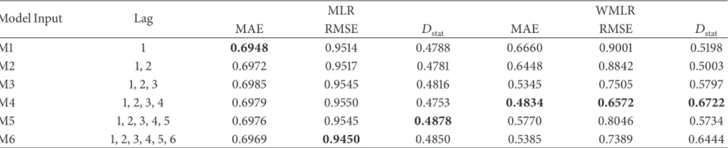
The forecasting performances of the MLR and WMLR

models in terms of the MAE, RMSE, and𝐷stattesting phase

are compared and shown in Table 2. Table 2 shows MLR

model; the M1 with 1 lag obtained the best MAE statistics of 0.6948 and the M6 with 6 lags obtained the best RMSE statistics of 0.9450, while the M1 with 5 lags obtained the best

(6)

GARCH ARIMA WMLR MLR 5 0 Er ro r −5 −10

Figure 5: The errors of MLR, WMLR, ARIMA, and GARCH models for crude oil price forecasting.

Table 2: Forecasting performance indices of MLR and WLR.

Model Input Lag MLR WMLR

MAE RMSE 𝐷stat MAE RMSE 𝐷stat

M1 1 0.6948 0.9514 0.4788 0.6660 0.9001 0.5198 M2 1, 2 0.6972 0.9517 0.4781 0.6448 0.8842 0.5003 M3 1, 2, 3 0.6985 0.9545 0.4816 0.5345 0.7505 0.5797 M4 1, 2, 3, 4 0.6979 0.9550 0.4753 0.4834 0.6572 0.6722 M5 1, 2, 3, 4, 5 0.6976 0.9545 0.4878 0.5770 0.8046 0.5734 M6 1, 2, 3, 4, 5, 6 0.6969 0.9450 0.4850 0.5385 0.7389 0.6444

𝐷statstatistics of 0.4878. For WMLR, model M4 with 4 lags

obtained the best MAE, RMSE, and𝐷statstatistics of 0.4834,

0.6572, and 0.6722, respectively. The equations of MLR with six input variables and WMLR with four input variables, respectively, are ̂𝑦𝑡= − 0.025𝑦𝑡−1− 0.047𝑦𝑡−2+ 0.22𝑦𝑡−3 − 0.082𝑦_𝑡−4− 0.060𝑦_𝑡−5+ 0.0004𝑦_𝑡−6, 𝑟_𝑡= 0.076𝑧₁(𝑡) − 0.221𝑧₂(𝑡) − 0.213𝑧₃(𝑡) − 0.510𝑧₄(𝑡) + 0.416𝑧₅(𝑡) − 0.930𝑧₆(𝑡) , (17)

where 𝑧_𝑖(𝑡) are called principal components and ̂𝑦_𝑡 =

𝑦_𝑡−1exp(𝑟_𝑡).

For further analysis, the best performance of the LR, WMLR, ARIMA, and ARIMA-GARCH models was com-pared with the best results of ARIMA and forward neural

network (FNN) studied by Yu et al. [1]. In Table 3, it

shows that WMLR outperform MLR, ARIMA, GARCH, Yu’ ARIMA and Yu’ FNN models in terms of RMSE statistics. This results show that the new series (DWT) have significant extremely positive effect on MLR model results.

Figure 5 shows the Box-plot for the ARIMA, ARIMA-GARCH, MLR, and WMLR models for testing period. It can be seen that the errors of WMLR model are quite close to the zero. Overall, it can be concluded that the WMLR model provided more accurate forecasting results than the other models for crude oil forecasting.

Table 3: The RMSE and MAE comparisons for different models.

Model RMSE MAE

ARIMA (2, 1, 5) 1.3835 1.0207

GARCH (1, 1) 0.9513 0.6947

MLR 0.9450 0.6969

WMLR 0.6572 0.4834

Yu’ ARIMA (Yu et al., [1]) 2.0350 —

Yu’ FNN (Yu et al., [1]) 0.8410 —

4. Conclusions

The accuracy of the wavelet multiple linear regression (WMLR) technique in the forecasting daily crude oil has been investigated in this study. The PCA is used to choose the principle component scores of the selected inputs which were used as independent variables in the MLR model and the par-ticle swarm optimization (PSO) is used to adopt the optimal parameters of the MLR model. The performance of the pro-posed WMLR model was compared to regular LR, ARIMA, and GARCH model for crude oil forecasting. Comparison results indicated that the WMLR model was substantially more accurate than the other models. The study concludes that the forecasting abilities of the MLR model are found to be improved when the wavelet transformation technique is adopted for the data preprocessing. The decomposed periodic components obtained from the DWT technique are found to be most effective in yielding accurate forecast when used as inputs in the MLR model. The accurate forecasting results

(7)

indicate that WMLR model provides a superior alternative to other models and a potentially very useful new method for crude oil forecasting. The WMLR model presented in this study is a simple explicit mathematical formulation. The WMLR model is much simpler in contrast to ANN model and can be successfully used in modeling short-term crude oil price. In the present study, three resolution levels were employed for decomposing crude oil time series. If more resolution levels were used, the results from WMLR model may turn out better. This may be a subject of another study.

Conflict of Interests

The authors declare that there is no conflict of interests regarding the publication of this paper.

Acknowledgments

The authors thankfully acknowledged the financial support that was afforded by Universiti Teknologi Malaysia under GUP Grant (VOT 06J13). Besides that, the authors would like to thank the Department of Irrigation and Drainage, Ministry of natural Resources and Environment, Malaysia, in helping us to provide the data.

References

[1] L. Yu, S. Wang, and K. K. Lai, “Forecasting crude oil price with an EMD-based neural network ensemble learning paradigm,”

Energy Economics, vol. 30, no. 5, pp. 2623–2635, 2008. [2] H. Mohammadi and L. Su, “International evidence on crude

oil price dynamics: applications of ARIMA-GARCH models,”

Energy Economics, vol. 32, no. 5, pp. 1001–1008, 2010.

[3] M. I. Ahmad, “Modelling and forecasting Oman Crude Oil Prices using Box-Jenkins techniques,”International Journal of Trade and Global Markets, vol. 5, pp. 24–30, 2012.

[4] P. Agnolucci, “Volatility in crude oil futures: a comparison of the predictive ability of GARCH and implied volatility models,”

Energy Economics, vol. 31, no. 2, pp. 316–321, 2009.

[5] Y. Wei, Y. Wang, and D. Huang, “Forecasting crude oil market volatility: further evidence using GARCH-class models,”Energy Economics, vol. 32, no. 6, pp. 1477–1484, 2010.

[6] L. Liu and J. Wan, “A Study of Shangai fuel oil futures price volatility based on high frequency data: long-range dependence, modeling and forecasting,” Economic Modelling, vol. 29, pp. 2245–2253, 2012.

[7] A. Ghaffari and S. Zare, “A novel algorithm for prediction of crude oil price variation based on soft computing,”Energy Economics, vol. 31, no. 4, pp. 531–536, 2009.

[8] M. A. Kaboudan, “Compumetric forecasting of crude oil prices,” inThe Proceedings of IEEE Congress on Evolutionary Computa-tion, pp. 283–287.

[9] S. Mirmirani and H. C. Li, “A comparison of VAR and neural networks with genetic algorithm in forecasting price of oil,”

Advances in Econometrics, vol. 19, pp. 203–223, 2004.

[10] W. E. Shambora and R. Rossiter, “Are there exploitable ineffi-ciencies in the futures market for oil?”Energy Economics, vol. 29, no. 1, pp. 18–27, 2007.

[11] L. Yu, S. Wang, and K. K. Lai, “A novel nonlinear ensemble forecasting model incorporating GLAR and ANN for foreign

exchange rates,”Computers and Operations Research, vol. 32, no. 10, pp. 2523–2541, 2005.

[12] W. Xie, L. Yu, S. Y. Xu, and S. Y. Wang, “A new method for crude oil price forecasting based on support vector machines,”Lecture Notes in Computer Science, vol. 3994, pp. 441–451, 2006. [13] R. Jammazi and C. Aloui, “Crude oil price forecasting:

exper-imental evidence from wavelet decomposition and neural network modeling,”Energy Economics, vol. 34, no. 3, pp. 828– 841, 2012.

[14] W. Qunli, H. Ge, and C. Xiaodong, “Crude oil price forecasting with an improved model based on wavelet transform and RBF neural network,” inProceedings of the International Forum on Information Technology and Applications (IFITA ’09), pp. 231– 234, May 2009.

[15] S. Yousefi, I. Weinreich, and D. Reinarz, “Wavelet-based predic-tion of oil prices,”Chaos, Solitons and Fractals, vol. 25, no. 2, pp. 265–275, 2005.

[16] Y. Bao, X. Zhang, L. Yu, K. K. Lai, and S. Wang, “Hybridizing wavelet and least squares support vector machines for crude oil price forecasting,” inProceedings of the 2nd International Workshop on Intelligent Finance, Chengdu, China, 2007. [17] J. Liu, Y. Bai, and B. Li, “A new approach to forecast crude

oil price based on fuzzy neural network,” inProceedings of the 4th International Conference on Fuzzy Systems and Knowledge Discovery (FSKD ’07), pp. 273–277, August 2007.

[18] G. E. P. Box and G. M. Jenkins,Time Series Analysis: Forecasting and Control, Holden-Day, San Francisco, Calif, USA, 1976. [19] T. Bollerslev, “Generalized autoregressive conditional

het-eroskedasticity,”Journal of Econometrics, vol. 31, no. 3, pp. 307– 327, 1986.

[20] H. Bozdogan and J. A. Howe, “Misspecified multivariate regres-sion models using the genetic algorithm and information complexity as the fitness function,”European Journal of Pure and Applied Mathematics, vol. 5, no. 2, pp. 211–249, 2012. [21] S. M. Chen and P. Y. Kao, “TAEIX forecasting based on

fuzzy time series, partical swarm optimization techniques and support vector machines,”Information Sciences, vol. 247, pp. 62– 71, 2013.

[22] R. Alwee, S. M. Shamsuddin, and R. Sallehuddin, “Hybrid support vector regression and autoregressive integrated moving average models improved by particle swarm optimization for property crime rates forecasting with economic indicators,”The Scientific World Journal, vol. 2013, Article ID 951475, 11 pages, 2013.

[23] R. J. Ma, N. Y. Yu, and J. Y. Hu, “Application of particle swarm optimization algorithm in the heating system planning problem,” The Scientific World Journal, vol. 2013, Article ID 718345, 11 pages, 2013.

[24] G. Tyagi and M. Pandit, “Combined heat and power dispatch using time varying acceleration coefficient particle swarm opti-mazation,”International Journal of Engineering and Innovative Technology, vol. 1, no. 4, pp. 234–240, 2012.

[25] L. Liu, S. Yang, and D. Wang, “Particle swarm optimization with composite particles in dynamic environments,” IEEE Transactions on Systems, Man, and Cybernetics B: Cybernetics, vol. 40, no. 6, pp. 1634–1648, 2010.

[26] D. Bratton and J. Kennedy, “Defining a standard for particle swarm optimization,” inProceedings of the IEEE Swarm Intel-ligence Symposium (SIS ’07), pp. 120–127, IEEE Service Center, Piscataway, NJ, USA, April 2007.

(8)

[27] J. Kennedy and R. Eberhart, “Particle swarm optimization,” inProceedings of the IEEE International Conference on Neural Networks, pp. 1942–1948, December 1995.

[28] S. G. Mallat, “Theory for multiresolution signal decomposition: the wavelet representation,”IEEE Transactions on Pattern Anal-ysis and Machine Intelligence, vol. 11, no. 7, pp. 674–693, 1989. [29] H. Ç amdevýren, N. Demýr, A. Kanik, and S. Keskýn, “Use

of principal component scores in multiple linear regression models for prediction of Chlorophyll-a in reservoirs,”Ecological Modelling, vol. 181, no. 4, pp. 581–589, 2005.

[30] I. T. Jolliffe,Principal Component Analysis, Springer, New York, NY, USA, 1986.

(9)

Submit your manuscripts at

http://www.hindawi.com

Computer Games Technology International Journal of

Hindawi Publishing Corporation

http://www.hindawi.com Volume 2014

http://www.hindawi.com Volume 2014 Distributed Sensor Networks International Journal of Advances in

Fuzzy

Systems

International Journal of

Reconfigurable Computing

Applied

Computational

Intelligence and Soft

Computing

Advances in

Artificial

Intelligence

Hindawi Publishing Corporation http://www.hindawi.com Volume 2014 Advances in Software Engineering

Electrical and Computer Engineering

Journal of

Computer Networks and Communications

http://www.hindawi.com Volume 2014 Hindawi Publishing Corporation

http://www.hindawi.com Volume 2014

Multimedia

International Journal of

Biomedical Imaging

Artificial

Neural Systems

Advances in

Robotics

Journal of

http://www.hindawi.com Volume 2014 Hindawi Publishing Corporationhttp://www.hindawi.com Volume 2014 Computational Intelligence and Neuroscience

Modelling & Simulation in Engineering Hindawi Publishing Corporation

The Scientific

World Journal

Human-Computer Interaction

Advances in

Computer EngineeringAdvances in