1
Limited Random Walk Algorithm for Big Graph
Data Clustering
Honglei Zhang,
Member, IEEE,
Jenni Raitoharju,
Member, IEEE,
Serkan Kiranyaz,
Senior Member, IEEE,
and Moncef Gabbouj,
Fellow, IEEE
Abstract—Graph clustering is an important technique to understand the relationships between the vertices in a big graph. In this paper, we propose a novel random-walk-based graph clustering method. The proposed method restricts the reach of the walking agent using an inflation function and a normalization function. We analyze the behavior of the limited random walk procedure and propose a novel algorithm for both global and local graph clustering problems. Previous random-walk-based algorithms depend on the chosen fitness function to find the clusters around a seed vertex. The proposed algorithm tackles the problem in an entirely different manner. We use the limited random walk procedure to find attracting vertices in a graph and use them as features to cluster the vertices. According to the experimental results on the simulated graph data and the real-world big graph data, the proposed method is superior to the state-of-the-art methods in solving graph clustering problems. Since the proposed method uses the embarrassingly parallel paradigm, it can be efficiently implemented and embedded in any parallel computing environment such as a MapReduce framework. Given enough computing resources, we are capable of clustering graphs with millions of vertices and hundreds millions of edges in a reasonable time.
Index Terms—Graph Clustering, Random Walk, Big Data, Community Finding, Parallel Computing
F
1
INTRODUCTION
G
RAPHdata are important data types in many scientific areas, such as social network analysis, bioinformatics, and computer and information network analysis. Big graphs are normally heterogeneous. They have such non-uniform structures that edges between vertices in a group are much denser than edges connecting vertices in different groups. Graph clustering (also named as “community detection” in the literature) algorithms aim to reveal the heterogeneity and find the underlying relations between vertices. This technique is critical for understanding the properties, pre-dicting dynamic behavior and improving visualization of big graph data.Graph clustering is a computationally challenging and difficult task, especially for big graph data. Many algorithms have been proposed over the last decades [1]. The criteria-based approaches try to optimize clustering fitness functions using different optimization techniques. Newman defined a modularity measurement based on the probability of the link between any two vertices. He applied a greedy search method to minimize this modularity fitness function in order to partition a graph into clusters [2]. Blondel and Clauset used the same fitness function but combined it with other optimization techniques [3], [4], [5]. Spielman and Teng opted the graph conductance measurement as the
• Honglei Zhang, Jenni Raitoharju, and Moncef Gabbouj are with the Department of Signal Processing, Tampere University of Technology, Tampere, Finland
E-mail: honglei.zhang, jenni.raitoharju, [email protected].
• Serkan Kiranyaz is with the Electrical Engineering Department, College of Engineering, Qatar University, Qatar
E-mail: [email protected]
fitness function [6]. Other than criteria-based methods, spec-tral analysis has also been widely adapted in this area [7], [8]. Random-walk-based methods tackle the problem from a different angle [9], [10]. These methods use the Markov chain model to analyze the graph. Each vertex represents a state and the links indicate transitions between the states. The probability values that are distributed among the states (vertices) reveal the graph structure.
In recent years, the size of graph data has grown dra-matically. Furthermore, most graphs are highly dynamic. It is very challenging or even intractable to partition the whole graph in real-time. Very often, people are only in-terested in finding the cluster that contains a seed vertex. This problem is called local clustering problem [6], [11], [12]. For example, from an end user’s perspective, finding the closely connected friends around him or her is more important than revealing the global user clusters of a large social network. It is unnecessary to explore the whole graph structure for this problem. Recently, random walk methods have gained great attention on this local graph clustering problem, since a walk started from the seed vertex is more likely to stay in the cluster where the seed vertex belongs. Comparing to the criteria-based methods, the random-walk-based methods are capable of extracting local information from a big graph without the knowledge of the whole graph data. In [13], [14], [15], a random walk is first applied to find important vertices around the seed vertex. Then a sweep stage is involved to select the vertices that minimize the conductance of the candidate clusters.
The accuracy of any criteria-based clustering method (or those combined with the random walk procedures) is greatly affected by the chosen clustering fitness function. Furthermore, most local clustering algorithms use the crite-ria that are more suitable for the global graph clustering
problem. These choices greatly degrade the performance of these algorithms when the graph is big and highly un-even. Also the majority of the graph clustering algorithms are designed in sequential computing paradigm. Therefore, they do not take advantage of modern high-performance computing systems.
In this paper, we propose a novel random-walk-based graph clustering algorithm—the Limited Random Walk (LRW) algorithm. First of all, the LRW algorithm does not rely on any clustering fitness function. Furthermore, the proposed method can efficiently tackle the computational complexity using a parallel programming paradigm. Finally, as a unique property among many graph clustering meth-ods, the LRW can be adapted to both global and local graph clustering in an efficient way.
The rest of the paper is organized as follows: basics of the graph structure and the random walk procedure are explained in Section 2; the LRW procedure is explained and analyzed in Section 3; the proposed LRW algorithm for the global and local graph clustering problems are introduced in Section 4; an extensive set of experiments on the simulated and real graph data, along with both numerical and visual evaluations are given in Section 5; finally, the conclusions and future work are in Section 6.
2
BASIC
DEFINITIONS AND THE
RANDOM
WALK
PROCEDURE
Let G(V, E) denote a graph of n vertices and m edges, where V = {vi|i= 1, . . . n} is the set of vertices and
E = {ei|i= 1, . . . m} is the set of edges. LetA ∈ Rn×n be the adjacency matrix of the graph G and Aij are the elements in the matrix A. Let D ∈ Rn×n
be the degree matrix, which is a diagonal matrix whose elements on the diagonal are the degrees of each vertex. In this paper, we assume the graph is undirected, unweighted and does not contain self-loops.
Clustering phenomenon is very common in big graph data. A cluster in a graph is a vertex set where the density of the edges inside the cluster is much higher than the density of edges that link the inside vertices and the outside vertices. Random walk on a graph is a simple stochastic proce-dure. At the initial state, we let an agent stay on a chosen vertex (seed vertex). At each step, the agent randomly picks a neighboring vertex and moves to it. We repeat this movement and study the probability that the agent lands on each vertex.
Letx(it)denote the probability that the agent is on vertex
viafter stept, wherei= 1,2, . . . n.x
(0)
i is the probability of the initial state. Letsbe the seed vertex. We havex(0)s = 1, andx(0)i = 0fori6=s. Letx(t)= hx(1t), x(2t), . . . , x(nt)
iT be the probability vector, where the superscriptT denotes the transpose of a matrix or a vector. By the definition of the probability, it is easy to see thatPni=1x
(t) i = 1or x(t) 1= 1.
The random walk procedure is equivalent to a discrete-time stationary Markov chain process. Each vertex is cor-responding to a state in the Markov chain and each edge indicates a possible transition between the two states. The
Markov transition matrixP can be obtained by normalizing the adjacency matrix to have each column sum up to 1, e.g.
Pij = Aij Pn k=1Akj (1) or P =AD−1. (2)
Other forms of the transition matrixP can also be used, for example the lazy random walk transition matrix in which
P = 1
2(I+AD
−1)
. Given the transition matrixP, we can calculatex(t+1)fromx(t)using the equation:
x(t+1)=P x(t). (3) A closed walk is a walk on a graph where the ending vertex is same as the seed vertex. The period of a vertex is defined as the greatest common divisor of the lengths of all closed walks that start from this vertex. We say a graph is aperiodic if all of its vertices have periods of 1.
For an undirected, connected and aperiodic graph, there exists an equilibrium stateπ, such thatπ=P π. This state is unique and irrelevant to the starting point. By iterating Eq. 3,x(t)
converges toπ. More details about the Markov chain process and the equilibrium state can be found from [16].
3
LIMITED
RANDOM
WALK
PROCEDURE
3.1 Definitions
We first define the transition matrixP. We assign the same probability to the transition that the walking agent stays in the current vertex and the transition that it moves to any neighboring vertex. We add an identity matrix to the adjacency matrix and then normalize the result to have each column sum to1. The transition matrix can be written as
P = (I+A) (I+D)−1. (4) Comparing to the transition matrix in Eq. 2, this is similar to adding self-loops to the graph. But we increase the degree of each vertex by 1 instead of 2. This modification fixes the periodicity problem that the graph may have. It greatly improves the algorithm’s stability and accuracy in graph clustering.
At each walking step the probability vectorx(t)is
com-puted using Eq. 3. Note that, in general, elements in x(t)
that are around the seed vertex are non-zeros and the rest are zeros. So we do not need the full transition matrix to calculate the probability vector for the next step.
Starting from the seed vertex, a normal random walk procedure will eventually explore the whole graph. To re-veal a local graph structure, different techniques can be used to limit the scope of the walks. In [10] and [13], the random walk function is defined as
x(t+1)=αx(0)+ (1−α)P x(t), (5) where αis called the teleport probability. The idea is that there is a certain probability that the walking agent will teleport back to the seed vertex and continue walking.
Inspired by the Markov Clustering Algorithm (MCL) algorithm [9], we adapt the inflation and normalization operation after each step of the transition. The inflation op-eration is an element-wise super-linear function—a function
3 that grows faster than a linear function. Here we use the
power function
f(x) = [xr1, xr2, . . . , xrn]T, (6) where the exponentr >1.
Sincexindicates the probability that the agent hits each vertex,xmust be normalized to have a sum of 1 after the inflation operation. The normalization function is defined as
g(x) = x
kxk1, (7)
wherekxk1=Pni=1|xi|is theL1norm of the vectorx. Since
xi≥0and Pn
i=1xi= 1, Eq. 7 can also be written in a vector form as
g(x) = x
xT·1, (8)
where 1 = [1,1, . . .1]T. The inflation and normalization operation enhance large values and depress small values in the vectorx.
We call this procedure the Limited Random Walk (LRW) procedure. The procedure limits the agent to walk around the neighborhood of the seed vertex, especially if there is a clear graph cluster boundary.
The MCL algorithm simulates flow within a graph. It uses the inflation and normalization operation to enhance the flow within a cluster and reduce the flow between clus-ters. The MCL procedure is a time-inhomogeneous Markov Chain in which the transition matrix varies over time. The MCL algorithm starts the random walk from all vertices simultaneously—there are n agents walking on the graph at the same time. The walking can only continue after all agents have completed a walking step and the result proba-bility matrix has been inflated and normalized. Unlike in the MCL algorithm, the LRW procedure is a time-homogeneous Markov Chain. We initiate random walk from a single seed vertex, and do the inflation on the probability values of this walking agent. This design has many advantages. First, it avoids unnecessary walks since the graph structure around the seed vertex may be exposed by a single walk. Second, the procedure is suitable for the local clustering problems because it does not require the whole graph data. Third, if multiple walks are required, each walk procedure can be executed independently. Thus the algorithm is fully parallelizable.
The LRW procedure involves a nonlinear operation, thus it is difficult to analyze its properties on a general graph model. Next we study the equilibrium of the LRW procedure. Later, we will use these properties to analyze the LRW procedure on general graphs.
3.2 Equilibrium of the LRW procedure
We first prove the existence of equilibrium of the LRW procedure. Let X be the set of values of the probability vectorx. We have
X = {(x1, x2,· · ·, xn)|0≤x1, x2,· · ·, xn ≤1 andx1+x2+· · ·xn= 1}. (9) The LRW procedure defined by Eqs. 3, 6 and 7 is a function that mapsX to itself. LetL: X →X, such that
L(x) =g(f(P x)). (10)
Theorem 1. There exists a fixed-pointx∗such thatL(x∗) =x∗. Proof: We use the Brouwer fixed-point theorem to prove this statement.
Given 0 ≤ x1, x2,· · ·, xn ≤ 1, the set X is clearly bounded and closed. ThusXis a compact set.
Let u, v ∈ X and w = λu+ (1−λ)v, where λ ∈ R
and0≤λ≤1. So wi =λui+ (1−λ)vifori = 1,2,· · ·n. Obviously0≤wi≤1. Further, n X i=1 wi = n X i=1 (λui+ (1−λ)vi) = λ n X i=1 ui+ (1−λ) n X i=1 vi = 1
Thusw∈X. This indicates that the setXis convex. Since function f(x) is continuous over the set X and functiong(x)is continuous over the codomain of function
f(x), functionLis continuous over the setX.
According to the Brouwer fixed-point theorem, there is a pointx∗such thatL(x∗) =x∗.
Theorem 1 shows the existence of fixed-point of the LRW procedure, i.e., the LRW procedure will not escape from a fixed-point whenever the point is reached. Since the LRW procedure is a non-linear discrete dynamic system, it is difficult to analytically investigate the system behavior. However, when r = 1, the LRW procedure is simply a Markov chain process, in which the fixed-point x∗ is the unique equilibrium state π and the global attractor. In another extreme case when r → ∞, a fixed-point can be an unstable equilibrium and the LRW procedure may have limit cycles that oscillate around a star structure in the graph. In one state of the oscillation, the probability value of the center of a star structure is close to one. In practice, we chose r from(1,2], where the LRW procedure is close to a linear system and oscillations are extremely rare. In this case, the fixed-points of the LRW procedure are stable equilibriums.
Next we show how to use the LRW procedure to find clusters in a graph.
3.3 Limited Random Walk on General Graphs
Without any prior knowledge of the cluster formation, we normally start the LRW procedure from an initial state where xs = 1,xi = 0for i 6= s and sis the seed vertex. During the LRW procedure, there are two simultaneous processes—the spreading process and the contracting pro-cess. When the two processes can balance each other, the stationary state is reached.
During the spreading process, the probability values spread as the walking agent visits new vertices. The num-ber of visited vertices increases exponentially at first. The growth rate depends on the average degree of the graph. The newly visited vertices will always receive the smallest probability values. If the graph has an average degree ofd, it is not difficult to see that the expected probability value of a newly visited vertex at stept is(1/d)t. As the walking
continues, the probability values tend to be distributed more evenly among all visited vertices.
The other ongoing process during the LRW procedure is the contracting process. During this process, the probability values of the visited vertices contract to some vertices. Since the graph is usually heterogeneous, some vertices (and groups of vertices) will receive higher probability values as the procedure continues. The inflation operation further enhances this contracting effect. The degrees of a vertex and its surrounding vertices determine whether the probability values concentrate to or diffuse from these vertices. Some vertices, normally the center of a star structure, receive larger probability values than others. We call these vertices feature vertices since they can be used to represent the structure of a graph.
Because the density of edge inside a cluster is higher than that of linking the nodes inside and outside the cluster, the probability that a walking agent visits nodes outside the cluster is small. Thus, the LRW procedure will find feature vertices that the seed vertex belongs to. We can use these vertices as features to cluster the vertices.
The larger the inflation exponentris, the faster the algo-rithm converges to the feature vertices. The LRW procedure tries to find the feature vertices that are near the seed vertex. However, ifris too large, the probability values concentrate to the nearest feature vertex (or the seed vertex itself) before the graph is sufficiently explored. Ifris too small, the prob-ability values will concentrate to the feature vertices that may belong to other clusters. The performance of the LRW algorithm depends on choosing a proper inflation exponent
r. From this aspect, it is similar to the MCL algorithm. In practice,ris normally chosen between1and2and the value 2was found to be suitable for most graphs.
4
LIMITED
RANDOM
WALK FOR
GRAPH
CLUSTER-ING
PROBLEMS
4.1 Global Graph Clustering Problems
In this section we use the proposed LRW procedure in global graph clustering problems. Our algorithm is divided into two phases—graph exploring phase and cluster merging phase. To improve the performance on big graph data, we also introduce a multi-stage strategy.
4.1.1 Graph Exploring Phase
In the graph exploring phase, the LRW procedure is started from several seed vertices. At each iteration, the agent moves one step as defined in Eq. 3. Then the probability vectorxis inflated by Eq. 6 and normalized by Eq. 7. The iteration stops when the probability vectorxconverges or the predefined maximum number of iterations is reached. Let x(∗,i) denote the final probability vector of a random
walk that was started from the seed vertexvi. As described in the previous section, the LRW procedure explores the vertices that are close to the seed vertex. Thus, the vector
x(∗,i)
has non-zero elements only on these neighboring vertices.
Algorithm 1 illustrates the graph exploring from a seed vertex setQ. Note that for small graph data, we can set the seed vertex setQ=V (i.e. the whole graph). In such case, the LRW procedure is executed on every vertex of the graph and the multi-stage strategy is not used.
Algorithm 1Limited random walk graph exploring from a vertex set
given adjacency matrix A of the graph G(V, E), the seed vertex set Q, the exponent r of the inflation function 6, maximum number of iterations Tmax, a small value to limit the number of visited vertices, and a small valueξfor the termination condition
initializethe transition matrixPby Eq. 4
for eachvertexiin the vertex setQ
1) initialize x(0,i) such that x(0k,i) = ( 1 k=i 0 otherwise andt= 1 2) repeat ift < Tmax a) x(t,i)=P x(t−1,i)
b) ifx(kt,i)< , setx(kt,i)to 0 c) x(kt,i)=f(xk(t,i)) =x(kt,i)
r d) x(kt,i)= x (t,i) k kx(t,i)k 1 e) ifx(t,i)−x(t−1,i)
2< ξ, exit the loop 3) outputx(t,i)as the feature vectorx(∗,i)for vertexi
Note that the threshold limit the number of nonzero elements in the probability vectorx. It is easy to prove that the number of nonzero elements in x(t,i) is less than 1/.
A largereliminates very small values inx(t,i)and prevent unnecessary computing efforts. However,does not impose a limit on the largest cluster we can find. Further, the choice ofhas little impact on the final clustering results because either the LRW procedure finds the most dominant feature vertices in a cluster or the small clusters are merged in the cluster merging phase.
4.1.2 Cluster Merging Phase
After the graph has been explored, we will find the clusters in the cluster merging phase. We treat each x(∗,i) as the
feature vector for the vertex vi. Vertices belonging to the same cluster have feature vectors that are close to each other. Any unsupervised clustering algorithm, such as k-means or single linkage clustering method, can be applied to find the desired number of (k) clusters. Because of the computational complexity of these clustering algorithms, we design a fast merging algorithm that can efficiently cluster vertices according to their feature vectors.
Each element x(j∗,i) in x(∗,i) is the probability value of the stationary state that the walking agent hits the vertex
vj when the seed vertex isvi. The feature vectorx(∗,i) is determined by the graph structure of the cluster that the initial vertexvibelongs to. Thus, vertices in the same cluster should have very similar feature vectors. We first find the vertex that has the largest value in the vectorx(∗,i)
. Suppose
m = arg maxjx(j∗,i), we call vm the attractor vertex of vertexvi. Grouping vertices by their attractor vertex can be done in a fast way (complexity ofO(1)) using a dictionary data structure. After the grouping, each vertex is assigned to a cluster that is identified by the attractor vertex. However, it is possible that some vertices in one cluster do not belong
5 to the same attractor vertex. This may happen when the
cluster is large and the edge density in the cluster is low. We then apply the following cluster merging algorithm to handle this overclustering problem.
The vertices that have large values, which determined by a threshold relative tox(m∗,i), inx(∗,i) are called significant vertices for vertex vi. If two vertices have large enough overlaps of their significant vertices, they should be grouped into the same cluster. From this observation, we first collect significant vertices for the found clusters. Then we merge clusters if their significant vertices overlap more than a half. Details of determining the significant vertices and merging clusters are given in
Note that the attractor vertex and the significant vertices are always in the same cluster as the seed vertex. This is very useful when we use the multi-stage graph strategy.
Algorithm 2 shows the details of the merging phase of the LRW algorithm. Note that, for small graph data, we set the seed vertex set Q=V and the initial clustering dictionary
Dto be empty.
Algorithm 2LRW cluster merging phase
givenfeature vectorsx(i∗,i)of the seed vertex setQ, where
i∈Q, thresholdτsuch that0< τ <1, and initial clustering dictionaryD
for eachfeature vectorx(i∗,i)wherei∈Q
1) find m = arg maxj(x(j∗,i))and add i to an empty vertex setS
2) find alljsuch thatxj(∗,i) > τ·x(m∗,i) and add them to an empty vertex setF
3) ifDdoes not contain the keym
add the pair hS,F i as the value that associated with the keymto dictionaryD
else
find the value hSm,Fmi that is associated with the keym
addi to set Sm and mergeF to Fm by Fm =
Fm∪ F
update the valuehSm,Fmi of the key m in the dictionaryD.
end
for eachpair of keysm1andm2in the dictionaryD
1) get the value pairs of hSm1,Fm1i and hSm2,Fm2i
that are associated with the keym1andm2
2) get the union of the significant vertex set of the two clusters byU =Fm1∩ Fm2
3) if|U |>12min (|Fm1|,|Fm2|)
a) mergeSm2toSm1 ,Sm1 =Sm1∪ Sm2
b) mergeFm2 toFm1,Fm1 =Fm1∪ Fm2
c) updatehSm1,Fm1ito the keym1
d) delete the keym2and its associated value
for eachkeyminD, outputSmas the clustering result
4.1.3 Multi-stage Strategy
For small graph data, we can do LRW procedure on every vertex of the graph. So the seed vertex setQ=V. The graph
clustering is completed after a graph exploring phase and a cluster merging phase. However, when the graph data is large, it is time-consuming to perform the LRW procedure from every vertex of the graph. A multi-stage strategy can be used to greatly reduce the number of required walkings. First, we start the LRW procedure from a randomly selected vertex set. After the first round of the graph exploring, some clusters can be found after the cluster merging phase. Next we generate a new seed vertex set by randomly selecting vertices from those vertices that have not been clustered. Then we do the graph exploration from the new seed vertex set. We repeat this procedure until all vertices are clustered. Algorithm 3 shows the global graph clustering algorithm using the multi-stage strategy.
Algorithm 3Global graph clustering algorithm using multi-stage strategy
given adjacency matrix A of the graph G(V, E), the ex-ponent r for the inflation function 6, threshold value η, maximum number of iterations Tmax and a small enough value
initializethe transition matrixPby Eq. 4, vertex setB=V
and clustering dictionaryD=∅
whileB is not empty
1) generate a vertex set Q ⊂ B by randomly select vertices fromB
2) do the graph exploring from the vertex setQusing algorithm 1 to get feature vectorsx(∗,i)fori∈Q
3) givenx(∗,i)andD, do the graph cluster merging
us-ing algorithm 2 to update the clusterus-ing dictionary
D
4) for each keymin D, merge the feature vertex set
Fmto the cluster vertex setSm,Sm=Sm∪ Fm 5) get clustered vertex setR=S
m∈DSm 6) letB=B\R
for eachkeyminD, outputSmas the clustering result
4.2 Local Graph Clustering Problems
For the local graph clustering problems, the LRW procedure can efficiently find the cluster from a given seed vertex. To achieve this, we first perform graph exploring from the seed vertex in the same way as described in Section 4.1.1. Letx(∗)
be the probability vector after the graph exploration. If a probability value inx(∗)is large enough, the corresponding
vertex is assigned the local cluster without further computa-tion. Similar to the global graph clustering algorithm, we use a relative thresholdηthat is related to the maximum value in x(∗)
. Vertices whose probability values are greater than
η·maxx(j∗)are called significant vertices. The significant vertices are assigned to the local cluster directly. A small value of η will reduce the computational complexity, but may decrease the accuracy of the algorithm. Suitable values ofηwere experimentally found to be between0.3and0.5.
The vertices with low probability values can either be outside of the cluster or inside the cluster but with rela-tively low significance. Unlike [6], [11], [12], which involve a sweep operation and a cluster fitness function, we do another round of graph exploring from these insignificant
vertices. After the second graph exploring is completed, we apply the cluster merging algorithm described in Section 4.1.2.
Algorithm 4 presents the LRW local clustering algorithm.
Algorithm 4LRW local graph clustering algorithm
givengraphG(V, E), seed vertexvand a threshold valueη,
where0< η <1
1) do graph exploration starting from the seed vertex
v as described in algorithm 1 and get the feature vectorx(∗,v)
2) find vertices in x(∗,v) for which x(∗,v)
i > 0 and collect the vertices in to setS
3) findm= arg maxj(x(j∗,v))
4) split the setSinto two setsS1andS2such thatS1=
n j|x(j∗,v)≥ηx(m∗,v) o andS2= n j|x(j∗,v)< ηx(m∗,v) o
5) for each vertex in S2 do graph exploration to get
feature vectorsx(∗,i)
, wherei∈S2
6) do clustering merging according to the feature vec-tors of the vertex v and the vertices in S2 as
de-scribed in algorithm 2 and find the cluster S3 that
contains the seed vertexv
7) returnS1∪S3
4.3 Computational Complexity
We first analyze the computational complexity of the LRW algorithm for the global graph clustering problem. We as-sume the graphG(V, E)has clusters. Letn¯cbe the average cluster size—the number of vertices in the cluster, andCis the number of clusters. We haven¯c·C =n. NoteC n. The most time-consuming part of the algorithm is the graph exploring phase. For each vertex, every iteration involves a multiplication of the transition matrixPand the probability vector x. The LRW procedure visits not only the vertices in the cluster but also a certain amount of vertices close to the cluster. Let γ be the coefficient that indicates how far the LRW procedure explores the graph before it con-verges. Notice the maximum number of nonzero elements in a probability vector is 1/. Let J denote the number of
vertices that the LRW procedure visits in each iteration, thus
J = min (γn¯c,1/). Thus the transition step at each iteration has complexity ofO(Jn¯c). The inflation and normalization steps, which operate on the probability vector x, have the complexity of O(J). Let K be the number of iterations for the LRW procedure to converge. So, the computational complexity for a complete LRW procedure on each vertex is
O(KJn¯c). For a global clustering problem when performing the LRW procedure on every vertex, the graph exploration phase has a complexity ofO(KJn¯cn). In the worst case, the algorithm has a complexity ofO n3. This is an extremely rare case and it only happens when the graph is small; does not have a cluster structure; and the edge density is high. This worst case scenario is identical to the MCL algorithm [9]. Notice that the variablesJ andK have upper bounds and ¯nc is determine by the graph structure, the algorithm has a complexity ofO(n)for big graph data.
The computational complexity of the cluster merging phase involves merging clusters that were found using the
attractor vertices. This merging requires C2
sets compar-ison operations, where C is the number of clusters found by the attractor vertices. The complexity of this phase is roughlyO(C2). This does not impose a significant impact
to the overall complexity of the algorithm, since C n. The time spent in this phase is often negligible. Experiments show that the clusters found using the attractor vertices are close to the final results. For applications where speed is more important than accuracy, the cluster merging phase can be left out.
When the LRW algorithm is used in local graph cluster-ing problem, the first graph exploration (started from the seed vertex) has a complexity of O(KJn¯c). After the first graph exploration, there are LJ vertices to be further ex-plored, whereLis related to the thresholdηandL <1. The overall complexity of the LRW local clustering algorithm is thusO(LKJ2¯nc).
The LRW algorithm is a typical example of embarrass-ingly parallel paradigm. In the graph exploring phase, each random walk can be executed independently. Therefore it can be entirely implemented in a parallel computing en-vironment such as a high-performance computing system. The time spent for graph exploring phase decreases roughly linearly with respect to the number of available computing resources. The two-phase design also fits the MapReduce programming model and can easily be adapted into any MapReduce framework [17].
5
EXPERIMENTS
The LRW algorithm uses the following parameters: inflation exponent r, maximum number of iterations Tmax, small value, merging thresholdτ and local clustering threshold
η. In practice, except the inflation exponent r, the values of the other parameters have little impact to the final re-sults. The inflation power r should be chosen according to the density of the graph. A sparse graph should use a smaller value of r, thoughr = 2is suitable for most real world graphs. In our experiments, we chose r = 2 unless otherwise specified. The other parameters have been set as:
Tmax= 100, = 10−5andτ =η = 0.3. We will show the impact of some parameters in Section 5.4.
5.1 Simulated Data for Global Graph Clustering Prob-lem
We first show the performance of the LRW algorithm using simulated graph data. The simulated graph is generated using the Erdos-Renyi model [18] with some modifications to generate clusters. Using the ground truth of the cluster structure, we can evaluate the performance of graph clus-tering algorithms. This kind of simulated data are widely used in the literature [2], [19], [20], [21].
The graphs are generated by the model G(n, p, c, q) where c is the number of clusters, n is the number of vertices,pis the probability of the link between two vertices, andq=din/doutis the parameter that indicates the strength of the cluster structure, wheredinis the expected number of edges linking one vertex to other vertices inside the same cluster, and dout is the expected number of edges linking a given vertex to other vertices in other clusters. Larger
7
q indicates stronger cluster structure. When q = 1, each vertex has equal probability that it links to vertices that are inside and outside of the cluster—the graph has a very weak cluster structure. Letdbe the expected of degree of a vertex. So,d = din+dout = p(n−1). We use this model to generate graphs that consist ofcclusters and each cluster has the same number of vertices. For each pair of vertices, we link them with the probability (qqpc+1)((nn−−1)c) if they belong to the same cluster, and the probability ofn(pcq+1)((n−c1)−1)if they belong to different clusters.
We use the normalized mutual information (NMI) to evaluate the clustering result against the ground truth [22], [23]. We first calculate the confusion matrix where each row is a cluster found by the clustering algorithm and each column is a cluster in the ground truth. The entries in the confusion matrix are the cardinality of the intersect set of the row cluster and the column cluster. LetNijbe the value of the i-th row and j-th column, Ni− the sum of thei-th row,N−j the sum of thej-th column,N the total number of vertices, CA the number of clusters that the clustering algorithm found (number of rows), andCG the number of clusters in the ground truth (number of columns). The NMI is calculated as follows: N M I = −2 PCA i=1 PCG j=1Nijlog (NijN/Ni−N−j) PCA i=1Ni−log (Ni−/N) + PCG j=1N−jlog (N−j/N) , (11) where0≤N M I≤1.
If the clustering algorithm returns the exact same cluster structure as the ground truth, N M I = 1. Notice, NMI is not a symmetric evaluation metric. If an algorithm assigns all vertices into one cluster (CA = 1), then NMI value is0. On the other hand if an algorithm assigns each vertex to its own cluster (CA=N), thenN M I >0.
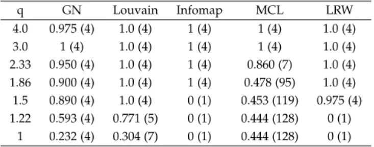
We generated graphs by choosingn= 128andd= 16. The number of the generated clusters is 4 and each cluster contains 32 vertices. We varied the ratio q and evaluated the performance of the LRW algorithm against Girvan-Newman (GN) [21], Louvain [3], Infomap [24] and MCL [9] algorithms. Two simulated graphs are shown in Fig. 1, where the clusters are colored differently and the graphs are visualized by force-directed algorithms.
(a) (b)
Fig. 1. Simulated graphs. (a)q= 4, (b)q= 1.22
The comparative results are given in Table 1, where the number of clusters found by the algorithms are placed between parentheses.
TABLE 1
The NMI Values and the Numbers of Clusters of the Clustering Results on Simulated Graph Data
q GN Louvain Infomap MCL LRW 4.0 0.975 (4) 1.0 (4) 1 (4) 1 (4) 1.0 (4) 3.0 1 (4) 1.0 (4) 1 (4) 1 (4) 1.0 (4) 2.33 0.950 (4) 1.0 (4) 1 (4) 0.860 (7) 1.0 (4) 1.86 0.900 (4) 1.0 (4) 1 (4) 0.478 (95) 1.0 (4) 1.5 0.890 (4) 1.0 (4) 0 (1) 0.453 (119) 0.975 (4) 1.22 0.593 (4) 0.771 (5) 0 (1) 0.444 (128) 0 (1) 1 0.232 (4) 0.304 (7) 0 (1) 0.444 (128) 0 (1)
From the results, Louvain the best performing algorithm and LRW algorithm comes as the second. It can be seen that the LRW algorithm can find the correct structure if the graph has a strong clustering structure. When the clustering structure diminishes as q decreases, the LRW algorithm returns the whole graph as one cluster. This behavior is beneficial when we need to find the true clusters in a big graph. The GN and Louvain algorithms are more like graph partition algorithms. They optimize certain cluster fitness functions using the whole graph data. They tend to partition the graph into clusters even though the cluster structure is weak.
We use real graph data to evaluate the performance of the LRW global clustering algorithm on heterogeneous graphs. Details of the experiments and the results are in Section 5.3.
5.2 Simulated Data for Local Graph Clustering Prob-lems
In this section, we compare the LRW algorithm with other local clustering algorithms. The test graphs are generated using the protocol defined in [20]. To simulate the data that are close to real world graphs, the vertex degree and the cluster size are chosen to follow the power law. Each test graph contains 2048 nodes. The vertex degree has the minimum value of 16 and the maximum value of 128. The minimum and maximum cluster size are 16 and 256, respectively. Similar to the previous section, the inbound-outbound ratioqdefines the strength of the cluster structure. The competing algorithms are criteria-based algorithms that optimize a fitness function using either the greedy search or the simulated annealing optimization method. Let
C be the cluster that contains the seed vertex. C¯= V\C is the complement vertex set ofC. Let functiona(·)be the total degree of a vertex set, that is
a(S) = X i∈S,j∈V
Aij, (12)
whereAijare the entries of the adjacency matrix. The cut of the clusterCis defined as
c(C) = X i∈C,j∈C¯
Aij. (13)
The following are the definitions of the fitness functions. Cheeger constant (conductance):
f(C) = c(C)
Normalized cut:
f(C) = c(C)
a(C)+
c(C)
a C¯ (15)
Inverse relative density:
f(C) =|E| −a(C) +c(C)
a(C)−c(C) (16) Different local clustering algorithms are used to find the cluster that contains the seed vertex. The Jaccard index is used to evaluate the performance of each algorithm. Let
C be the set of vertices that an algorithm finds andT be the ground truth cluster that contains the seed vertex. The Jaccard index is defined as
J= |C ∩ T |
|C ∪ T | (17)
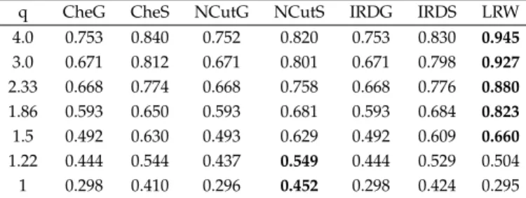
We generated 10 test graphs for each inbound-outbound ratio q. From each generated graph, we randomly picked 20 vertices as seeds. For each algorithm and each inbound-outbound ratioq, we computed the Jaccard index for each seed and took the average of the 200 Jaccard indices. The results are shown in Table 2, where “Che” stands for the Cheeger constant (conductance) fitness function; “NCut” stands for the normalized cut fitness function; “IRD” stands for the inverse relative density; the ending letter “G” stands for the greedy search method; and the ending letter “S” stands for the simulated annealing method.
TABLE 2
Jaccard Index of Local Graph Clustering Results on the Simulated Graphs
q CheG CheS NCutG NCutS IRDG IRDS LRW 4.0 0.753 0.840 0.752 0.820 0.753 0.830 0.945 3.0 0.671 0.812 0.671 0.801 0.671 0.798 0.927 2.33 0.668 0.774 0.668 0.758 0.668 0.776 0.880 1.86 0.593 0.650 0.593 0.681 0.593 0.684 0.823 1.5 0.492 0.630 0.493 0.629 0.492 0.609 0.660 1.22 0.444 0.544 0.437 0.549 0.444 0.529 0.504 1 0.298 0.410 0.296 0.452 0.298 0.424 0.295
From the results, the LRW algorithm greatly outperforms other methods when the graph has a clear cluster structure.
5.3 Real World Data
In this section, we evaluate the performance of the LRW algorithm on some real world graph data.
5.3.1 Zachary’s Karate Club
We first do clustering analysis on the Zachary’s karate club graph data [25]. This graph is a social network of friendship in a karate club in 1970. Each vertex represents a club mem-ber and each edge represents the social interaction between the two members. During the study, the club split into two smaller ones due to the conflicts between the administrator and the coach. The graph data have been regularly used to evaluate the performance of the graph clustering algorithms [21], [24], [26]. The graph contains 34 vertices and 78 edges. We applied the LRW algorithm on this graph and the result
shows two clusters that are naturally formed. Fig. 2 shows the clustering result, where clusters are illustrated using different colors.
Fig. 2. Clustering result of the karate club graph data
As the figure shows, the LRW algorithm finds the two clusters of the Zachary’s karate club. Actually the two clusters perfectly match the ground truth—how the club was split in 1970.
Clustering results of GN, Louvain, Infomap and MCL algorithms are given in supplementary material.
5.3.2 Ego-Facebook Graph Data
The second data we used is the ego-Facebook graph data [27]. The social network website Facebook allows users to organize their friends into “circles” or “friends lists” (for example, friends who share common interests). This data was collected from volunteer Facebook users for researchers to develop automatic circle finding algorithms. Ego-network is the network of an end user’s friends. The ego-Facebook graph is a combination of ego-networks from 10 volunteer Facebook users. There are 4039 vertices and 88234 edges in the graph.
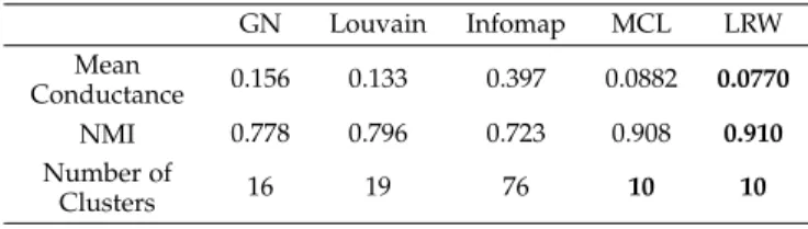
We applied the LRW, GN [21], Louvain [3], Infomap [24] and MCL [9] graph clustering algorithms to this data. To compare the results, we generated the ground truth clustering by combining the vertices in the “circles” of each volunteer user. So, the ground truth contains 10 clusters. If a vertex appears in the circles of more than one volunteer, we assign the vertex to all of these ground truth clusters. We evaluated the number of clusters and the NMI values of the results that each competing algorithm generates.
We also calculated the mean conductance (MC) value of the clustering results. The conductance value of a cluster is calculated using Eq. 14. We then take the mean of all the conductance values of the clusters that an algorithm finds. The smaller MC value shows better clustering results. Note that MC tends to favor smaller number of clusters in general. If the number of clusters are roughly same, MC values give good evaluation of the clustering results. It is also worth noting that MC value is capable of evaluating clustering algorithms without the ground truth. We shall use this metric in later experiments where the ground truth is not available.
The MC scores, NMI scores and the number of clusters found by each algorithm are reported in Table 3. A bold font indicates the best score among all competing algorithms.
9 TABLE 3
Global Graph Clustering Results on the Ego-Facebook Graph
GN Louvain Infomap MCL LRW Mean Conductance 0.156 0.133 0.397 0.0882 0.0770 NMI 0.778 0.796 0.723 0.908 0.910 Number of Clusters 16 19 76 10 10
The results show that the random-walk-based algorithms—LRW and MCL—are able to find the correct cluster structure of the data. Other criteria-based algorithms are sensitive to trivial disparities of the graph structure and are likely to overcluster the data.
The clustering result of the LRW algorithms is shown in Fig. 3.
Fig. 3. Clustering result on the ego-Facebook graph data
Clustering results of other algorithms are shown in the supplementary material.
5.3.3 Heterogeneous Graph Data
To evaluate the performance of the LRW algorithm on real heterogeneous graph data, we selected 5 graph data from the collection of the KONECT project [28]. The graph data are selected from different categories and the size of the graph data varies from small to medium. The properties and the references of the test graphs are shown in Table 4.
TABLE 4
Properties of the Testing Heterogeneous Graphs
Vertices Edges Category Reference dolphins 62 156 Animal [29] arenes-jazz 198 2742 Human Social [30] infectious 410 2765 Human Contact [31] polblogs 1490 19090 Hyperlink [32] reactome 6229 146160 Metabolic [33]
Since there is no ground truth available for these test data, we evaluated each clustering algorithm by the mean conductance (MC) values. The results are in Table 5. The best MC score are shown in a bold font. The numbers of clusters found by each algorithm are placed between parentheses. We also plot the clustered graphs in which the vertices are located using a force-directed algorithm
and colored according to their associated clusters. These clustered graphs are given in the supplementary material for subjective evaluation.
The reactome and the infectious graphs have low den-sity. We chose the inflation exponent r = 1.2 to prevent overclustering the data. For other graph data, the default valuer= 2is used.
TABLE 5
Global Graph Clustering Results on the Real Heterogeneous Graph Data GN Louvain Infomap MCL LRW dolphins 0.425 (4) 0.440 (5) 0.487 (6) 0.675 (12) 0.347 (4) arenes-jazz 0.485 (4) 0.455 (4) 0.577 (7) 0.529 (5) 0.364 (4) infectious 0.162 (5) 0.214 (6) 0.465 (17) 0.673 (40) 0.175 (5) polblogs 0.524 (12) 0.501 (11) 0.727 (36) 0.777 (45) 0.427 (11) reactome 0.108 (110) 0.099 (114) 0.315 (248) 0.478 (352) 0.221 (191)
Based on the MC scores and the visualized clustering results, the LRW algorithm achieves a superior clustering performance in most of the cases. Note that the reactome data has a weak cluster structure, thus the LRW algorithm has difficulty to find a good partition for it.
5.4 The Sensitivity Analysis of the Parameters
The proposed LRW algorithm depends on a number of parameters to perform global and local graph clustering. In this section, we perform the sensitivity analysis on the parameters.
We use both simulated and real-world graphs in our experiments. Test graph G1, G2 and G3 are similar to those used in Section 5.1 except that we vary the density of each graph. The expected degree d, which is a measure of the graph density, of graph G1, G2 and G3 are 12, 16 and 20 respectively andq is set to be 1.86 for all test graphs. Test graph G4 is generated in the same way as described in Section 5.2. The ego-Facebook graph data in Section 5.3.2 is used as an example of real-world graphs. We performed global graph clustering on these test graphs using the LRW algorithm with different parameters. NMI scores are used to evaluate the performance of the algorithm. The experiments using simulated graph data were repeated 10 times and the average NMI scores and the average number of clusters are reported.
As described in Section 3.3, the most important parame-ter of the LRW algorithm is the inflation exponentr. We first setTmax = 100, = 10−5,τ = 0.3 and vary the inflation exponent r. Table 6 shows NMI scores and the number of clusters reported by the LRW algorithm with different values ofr.
The test results show that the performance the LRW al-gorithm is sensitive to the density of the test graphs. A large inflation exponentrmay overcluster the data as the results on graph G1 and G2 shows. It can be easily noticed that the LRW algorithm is not sensitive to the choice of r for test graph G4 and the ego-Facebook graph. These graphs, and
TABLE 6
NMI Scores and the Number of Clusters by the Different Inflation Exponent Values r G1 G2 G3 G4 Facebook 1.2 (1)0 (1)0 (1)0 0.155(5) 0.902(10) 1.4 (1)0 (1)0 (1)0 (22.7)0.927 0.906(10) 1.6 (1)0 (1)0 (1)0 (23)1.0 0.908(11) 1.8 1 (4) 1 (4) 1 (4) 1.0 (20.8) 0.910 (10) 2 0.971 (4.6) 1 (4) 1 (4) 1.0 (25) 0.910 (10) 2.4 0.868 (7.0) 0.990 (4.2) 1 (4) 1.0 (21.8) 0.910 (10) 3 0.822 (6.3) 0.962 (4.8) 0.988 (4.2) 1.0 (24.3) 0.910 (10)
almost all real-world graphs, are more heterogeneous than the simulated graphs G1, G2 and G3. The LRW algorithm performs better on this type of graph since the attractor vertices and significant vertices are more stable on these graphs.
The parameter Tmax sets a limit on the number of iterations for the LRW procedure to converge. According to our experiments, value 100 is large enough to ensure the convergence of almost all cases. For example, only 3 out of 88,234 LRW procedures do not converge within 100 iterations on the ego-Facebook graph. A few exceptional cases has no impact on the final clustering results. The parameteris used to remove small values in the probability vector thus decrease the computational complexity. It has no impact on the final clustering result as long as the value is small enough, for example <10−4.
We also conducted the experiments by varying the threshold value τ from 0.1 to 0.5. The NMI scores and the number of clusters found by the LRW algorithm with different τ values are almost identical to those in Table 6. This indicates that the choice ofτ has very little impact on the clustering performance.
According to these results, one only needs to choose a proper inflation exponent rto use the LRW algorithms. Other parameters can be chosen freely from a wide range of reasonable values.r= 2is suitable for most of graphs and is preferable because of the computational advantage.
5.5 Big graph data
In this section, we apply the LRW algorithm on real-world big graph data and show the computational advantage of its parallel implementation. The test graphs were received from the SNAP graph data collection [34], [35]. These graphs are from major social network services and E-commerce companies. We use the high quality communities that either created by users or the system as ground truth clusters. The details of the high quality communities are described in [35]. The Rand Index is used to evaluate the results of the proposed clustering algorithm. To generate positive samples, we randomly picked 1000 pairs of vertices, where the vertices in each pair come from the same cluster in
the ground truth. Negative samples consist of 1000 pairs of vertices, where the vertices from each pair come from different clusters in the ground truth. The Rand Index is defined as
RI =T P +T N
N , (18)
whereT P is the number of true positive samples,T Nis the number of true negative samples, andNis the total number of samples.
Table 7 shows the size of the test graphs, the time spent on the graph exploration phase, the number of CPU cores and the amount of memory used for graph exploration, the time spent on cluster merging phase, the number of clusters that the LRW algorithm finds and the Rand Index of the clustering results. In this experiment, multiple CPU cores were used for graph exploration and one CPU core was used for clustering merging. Note that the competing algorithms used in previous sections cannot complete this task due to the large size of the data.
Table 7 shows that the LRW algorithm is able to find clusters from large graph data with a reasonable computing time and memory resource. The Rand Index values indicate that the clusters returned by the LRW algorithm match well the ground truth. The time spent on the graph exploration phase is inversely proportional to the number of CPU cores. Computational time can be further reduced if more computing resources are available. The proposed algorithm can efficiently handle graphs with millions of nodes and hundreds of millions of edges. For even larger graphs that exceed the memory limit for each computing process, a mechanism that retrieves part of the graph from a central storage can be used. Since the LRW procedure is capable of exploring a limited number of vertices that are near a seed vertex, the algorithm can cluster much larger graphs if such a mechanism is implemented.
6
CONCLUSIONS
In this paper, we proposed a novel random-walk-based graph clustering algorithm, the so-called LRW. We studied the behavior of the LRW procedure and developed the LRW algorithms for both global and local graph clustering prob-lems. The proposed algorithm is fundamentally different from previous random-walk-based algorithms. We use the LRW procedure to find attracting vertices and use them as features to cluster vertices in a graph. The performance of the LRW algorithm was evaluated using simulated graphs and real-world big graph data. According to the results, the proposed algorithm is superior to other well-known methods.
The LRW algorithm can be efficiently used in both global and local graph clustering problems. It finds clusters from a big graph data by only locally exploring the graph. This is important for extreme large data that may not even fit in a single computer memory. The algorithm contains two phases—the graph exploring phase and the cluster merging phase. The graph exploring phase is the most critical part and also the most time-consuming part of the algorithm. This phase can be implemented in embarrassingly parallel paradigm. The algorithm can easily be adapted to any MapReduce framework.
11 TABLE 7
Clustering Performance of Real-world Big Graph Data
com-Amazon com-Youtube com-LiveJournal com-Orkut nodes 334,863 1,134,890 3,997,962 3,072,441 edges 925,872 2,987,624 34,681,189 117,185,083 CPU cores for graph exploration 12 96 96 96
memory per CPU core 4G 4G 8G 8G graph exploration (in hours) 0.83 3.08 17.4 24.0
cluster merging (in hours) 0.20 1.34 9.44 2.53 clusters 37,473 170,569 381,246 165,624 Rand Index 0.908 0.755 0.951 0.751
From our experiments, we also noticed the limitation of the LRW algorithm. First, when used as a global clustering algorithm, the computational complexity can be high, espe-cially when the graph cluster structure is weak. This is due to the fact that the graph may be analyzed multiple times during the graph exploration phase, if we perform the LRW procedure from every vertex of the graph. However, using the multi-stage strategy can dramatically reduce the compu-tation time. Second, if the cluster structure is obscured, the LRW algorithm may return the whole graph as one cluster— though this behavior is desired in many cases.
The experiments show that the performance of the pro-posed LRW graph clustering algorithm is not sensitive to any parameter except the inflation exponent r, especially when the graph is not heterogeneous. For future research, we will further improve the LRW algorithm so that it can optimally select the inflation function that best suits the problem at hand.
REFERENCES
[1] S. E. Schaeffer, “Graph clustering,”Computer Science Review, vol. 1, no. 1, pp. 27–64, 2007.
[2] M. E. Newman, “Fast algorithm for detecting community structure in networks,”Physical review E, vol. 69, no. 6, p. 066133, 2004. [3] V. D. Blondel, J.-L. Guillaume, R. Lambiotte, and E. Lefebvre, “Fast
unfolding of communities in large networks,”Journal of Statistical Mechanics: Theory and Experiment, vol. 2008, no. 10, p. P10008, 2008. [4] A. Clauset, M. E. Newman, and C. Moore, “Finding community structure in very large networks,”Physical review E, vol. 70, no. 6, p. 066111, 2004.
[5] L. Waltman and N. J. v. Eck, “A smart local moving algorithm for large-scale modularity-based community detection,”The European Physical Journal B, vol. 86, no. 11, pp. 1–14, Nov. 2013.
[6] D. A. Spielman and S.-H. Teng, “A local clustering algorithm for massive graphs and its application to nearly-linear time graph partitioning,”arXiv preprint arXiv:0809.3232, 2008.
[7] H. Qiu and E. R. Hancock, “Graph matching and clustering using spectral partitions,”Pattern Recognition, vol. 39, no. 1, pp. 22–34, 2006.
[8] D. Spielman and S. Teng, “Spectral Sparsification of Graphs,”
SIAM Journal on Computing, vol. 40, no. 4, pp. 981–1025, Jan. 2011. [9] S. Dongen, “Graph clustering by flow simulation,” Ph.D.
disserta-tion, Universiteit Utrecht, Utrecht, The Netherlands, May 2000. [10] K. Macropol, T. Can, and A. K. Singh, “RRW: repeated random
walks on genome-scale protein networks for local cluster discov-ery,”BMC bioinformatics, vol. 10, no. 1, p. 283, 2009.
[11] F. Chung and M. Kempton, “A Local Clustering Algorithm for Connection Graphs,” inAlgorithms and Models for the Web Graph. Springer, 2013, pp. 26–43.
[12] P. Macko, D. Margo, and M. Seltzer, “Local clustering in prove-nance graphs,” inProceedings of the 22nd ACM international confer-ence on Conferconfer-ence on information & knowledge management. ACM, 2013, pp. 835–840.
[13] R. Andersen, F. Chung, and K. Lang, “Using pagerank to locally partition a graph,”Internet Mathematics, vol. 4, no. 1, pp. 35–64, 2007.
[14] T. Bühler, S. S. Rangapuram, S. Setzer, and M. Hein, “Constrained fractional set programs and their application in local clustering and community detection,”arXiv:1306.3409 [cs, math, stat], Jun. 2013.
[15] Z. A. Zhu, S. Lattanzi, and V. Mirrokni, “A local algorithm for find-ing well-connected clusters,” inProceedings of the 30th International Conference on Machine Learning (ICML-13), 2013, pp. 396–404. [16] J. Norris, “Markov Chains | Applied probability and stochastic
networks,” 1998.
[17] J. Dean and S. Ghemawat, “MapReduce: Simplified Data Process-ing on Large Clusters,”Commun. ACM, vol. 51, no. 1, pp. 107–113, Jan. 2008.
[18] M. Newman,Networks: An Introduction, 1st ed. Oxford ; New York: Oxford University Press, May 2010.
[19] L. Danon, A. Díaz-Guilera, and A. Arenas, “The effect of size heterogeneity on community identification in complex networks,”
Journal of Statistical Mechanics: Theory and Experiment, vol. 2006, no. 11, p. P11010, Nov. 2006.
[20] A. Lancichinetti, S. Fortunato, and F. Radicchi, “Benchmark graphs for testing community detection algorithms,”Physical Review E, vol. 78, no. 4, Oct. 2008.
[21] M. E. Newman and M. Girvan, “Finding and evaluating commu-nity structure in networks,” Physical review E, vol. 69, no. 2, p. 026113, 2004.
[22] L. Ana and A. Jain, “Robust data clustering,” in2003 IEEE Com-puter Society Conference on ComCom-puter Vision and Pattern Recognition, 2003. Proceedings, vol. 2, Jun. 2003, pp. II–128–II–133 vol.2. [23] L. Danon, A. Diaz-Guilera, J. Duch, and A. Arenas, “Comparing
community structure identification,”Journal of Statistical Mechan-ics: Theory and Experiment, vol. 2005, no. 09, p. P09008, 2005. [24] M. Rosvall and C. T. Bergstrom, “Maps of random walks on
complex networks reveal community structure,”Proceedings of the National Academy of Sciences, vol. 105, no. 4, pp. 1118–1123, Jan. 2008.
[25] W. W. Zachary, “An information flow model for conflict and fission in small groups,”Journal of anthropological research, pp. 452–473, 1977.
[26] T. Sahai, A. Speranzon, and A. Banaszuk, “Hearing the clusters of a graph: A distributed algorithm,”Automatica, vol. 48, no. 1, pp. 15–24, Jan. 2012.
[27] J. Leskovec and J. J. Mcauley, “Learning to Discover Social Circles in Ego Networks,” in Advances in Neural Information Processing Systems 25, F. Pereira, C. J. C. Burges, L. Bottou, and K. Q. Weinberger, Eds. Curran Associates, Inc., 2012, pp. 539–547. [28] J. Kunegis, “KONECT – The Koblenz Network Collection,” inProc.
Int. Conf. on World Wide Web Companion, 2013, pp. 1343–1350. [29] D. Lusseau, K. Schneider, O. J. Boisseau, P. Haase, E. Slooten, and
S. M. Dawson, “The bottlenose dolphin community of Doubtful Sound features a large proportion of long-lasting associations,”
Behavioral Ecology and Sociobiology, vol. 54, no. 4, pp. 396–405, Jun. 2003.
[30] P. Gleiser and L. Danon, “Community Structure in Jazz,”Advances in Complex Systems, vol. 06, no. 04, pp. 565–573, Dec. 2003. [31] L. Isella, J. Stehlé, A. Barrat, C. Cattuto, J.-F. Pinton, and
Behavioral Networks,”Journal of Theoretical Biology, vol. 271, no. 1, pp. 166–180, 2011.
[32] L. A. Adamic and N. Glance, “The Political Blogosphere and the 2004 U.S. Election: Divided They Blog,” inProceedings of the 3rd International Workshop on Link Discovery, ser. LinkKDD ’05. New York, NY, USA: ACM, 2005, pp. 36–43.
[33] D. Croft, A. F. Mundo, R. Haw, M. Milacic, J. Weiser, G. Wu, M. Caudy, P. Garapati, M. Gillespie, M. R. Kamdar, B. Jas-sal, S. Jupe, L. Matthews, B. May, S. Palatnik, K. Rothfels, V. Shamovsky, H. Song, M. Williams, E. Birney, H. Hermjakob, L. Stein, and P. D’Eustachio, “The Reactome pathway knowledge-base,”Nucleic Acids Research, p. gkt1102, Nov. 2013.
[34] J. Leskovec, “Stanford Large Network Dataset Collection.” [35] J. Yang and J. Leskovec, “Defining and Evaluating Network
Com-munities based on Ground-truth,”arXiv:1205.6233 [physics], May 2012.
Honglei Zhang is a PhD student and a re-searcher in the Department of Signal Process-ing at Tampere University of Technology. He re-ceived his Bachelor and Master degree in Elec-trical Engineering from Harbin Institute of Tech-nology in 1994 and 1996 in China, respectively. He worked as a software engineer in Founder Co. in China from 1996 to 1999. He had been working as a software engineer and a software system architect in Nokia Oy Finland for 14 years. He has 6 scientific publications and 2 patents. His current research interests include computer vision, pattern recognition, data mining and graph algorithms. More about of his re-search can be found from http://www.cs.tut.fi/~zhangh.
Jenni Raitoharju received her MS degree in information technology in 2009 from Tampere University of Technology and she’s now pursu-ing a PhD degree. She is currently workpursu-ing as a researcher at the Department of Signal Pro-cessing, Tampere University of Technology. Her research interests include content-based image analysis, indexing and retrieval, machine learn-ing, neural networks, stochastic optimization and divide and conquer algorithms.
Serkan Kiranyazwas born in Turkey, 1972. He received his BS degree in Electrical and Elec-tronics Department at Bilkent University, Ankara, Turkey, in 1994 and MS degree in Signal and Video Processing from the same University, in 1996. He worked as a Senior Researcher in Nokia Research Center and later in Nokia Mobile Phones, Tampere, Finland. He received his PhD degree in 2005 and his Docency at 2007 from Tampere University of Technology, respectively. He is currently a Professor in the Department of Electrical Engineering at Qatar University. Prof. Kiranyaz published 2 books, more than 30 journal papers in several IEEE Transactions and some other high impact journals and 70+ papers in international conferences. His recent publication has been nominated for the Best Paper Award in IEEE ICIP’13 conference. Another publication won the IBM Best Paper Award in ICPR’14.
Moncef Gabbouj received his BS degree in electrical engineering in 1985 from Oklahoma State University, and his MS and PhD degrees in electrical engineering from Purdue University, in 1986 and 1989, respectively. Dr. Gabbouj is cur-rently Academy of Finland Professor and holds a permanent position of Professor of Signal Pro-cessing at the Department of Signal ProPro-cessing, Tampere University of Technology. His research interests include multimedia content-based anal-ysis, indexing and retrieval, machine learning, nonlinear signal and image processing and analysis, voice conversion, and video processing and coding. Dr. Gabbouj is a Fellow of the IEEE and member of the Finnish Academy of Science and Letters. He is the past Chairman of the IEEE CAS TC on DSP and committee member of the IEEE Fourier Award for Signal Processing. He served as Distin-guished Lecturer for the IEEE CASS. He served as associate editor and guest editor of many IEEE, and international journals.