SENTIMENT ANALYSIS ON TWITTER DATA USING DIFFERENT ALGORITHMS
A Paper
Submitted to the Graduate Faculty of the
North Dakota State University of Agriculture and Applied Science
By
Monzuma Nazma
In Partial Fulfillment of the Requirements for the Degree of
MASTER OF SCIENCE
Major Program: Software Engineering
October 2018
North Dakota State University
Graduate School
TitleSENTIMENT ANALYSIS ON TWITTER DATA USING DIFFERENT ALGORITHMS By Monzuma Nazma
The Supervisory Committee certifies that this disquisition complies with North Dakota State University’s regulations and meets the accepted standards for the degree of
MASTER OF SCIENCE SUPERVISORY COMMITTEE: Dr. Simone Ludwig Chair Dr. Pratap Kotala
Dr. Maria de los Angeles Alfonseca-Cubero
Approved:
November 6, 2018 Dr. Kendall Nygard
ABSTRACT
Sentiment analysis is the process of determining opinion expressed in a text, or an
estimation of emotion related to the certain topic if it is negative, positive or neutral. The massive growth of social media, Twitter has played an important role since it allows people to express their feelings about a subject. Classification algorithms are necessary in the process of sentiment analysis. In this paper, we build a model to acquire people’s opinion on any concerning subject and evaluate the classification algorithms on the dataset. To accomplish the goal, we use a large set of Tweets which refer to a particular topic and execute the analytics on the Twitter feeds to classify them by using Naïve Bayes, Support Vector Machine, Maximum Entropy and Boosting algorithms. Then, to obtain the result we measure the accuracy among the four algorithms and compare them to identify the best algorithm based on our experiment.
ACKNOWLEDGEMENTS
I would like to express an immerse respect and sincere gratitude to my adviser, Dr. Simone Ludwig for her continued guidance, valuable suggestions, support, patience, and encouragement through the research process and giving me an opportunity to work under her guidance. I would also like to thank to my graduate committee member Dr. Pratap Kotala and Dr. Maria for their valuable time.
I would also like to thank my friend Susmit Sarkar for his inspiration, encouragement at every stage of my school and my work. Finally, I would like to thank my husband Md Arifin, my daughter & son Anika Arifin & Areeb Arifin, my parents and my other family members for their support, encouragement, inspiration, understanding and enduring blessing and love for me through the entire process.
DEDICATION
TABLE OF CONTENTS
ABSTRACT ... iii
ACKNOWLEDGEMENTS ... iv
DEDICATION ... v
LIST OF TABLES ... viii
LIST OF FIGURES ... ix
1. INTRODUCTION ... 1
2. RELATED WORK ... 3
3. METHODOLOGY ... 6
3.1. Overview of the Implementation ... 6
3.2. Creating a New Twitter App ... 8
3.3. Authorization to Access Twitter in “R” ... 10
3.4. Processing Text Twitter Feed in “R” ... 10
3.5. Sentiment Analysis with Classifiers ... 13
3.5.1. Naïve Bayes Classifier ... 13
3.5.1.1. Performance Evaluation ... 15
3.5.2. Support Vector Machine Classifier ... 17
3.5.3. Maximum Entropy Classifier ... 18
3.5.4. Boosting Classifier ... 19
4. EXPERIMENTS AND RESULTS ... 22
4.1. Dataset ... 22
4.2. Experiment with Naïve Bayes Classifier ... 22
4.2.1. Naïve Bayes Performance Evaluation ... 22
4.3.2. MaxEnt Performance Evaluation ... 24
4.3.3. Boosting Performance Evaluation ... 24
4.3.4. K-Fold Cross Validation... 25
4.3.4.1. 10-Fold Cross Validation for Naïve Bayes ... 25
4.3.4.2. 10-Fold Cross Validation for SVM... 27
4.3.4.3. 10-Fold Cross Validation for MaxEnt ... 28
4.3.4.4. 10-Fold Cross Validation for Boosting ... 29
4.3.5. Comparison... 29
4.3.5.1. Precision and Recall Comparison ... 30
4.3.5.2. Accuracy Comparison ... 30
4.3.5.3. F Measure Comparison for Four Classifiers ... 31
5. CONCLUSION AND FUTURE WORK ... 34
LIST OF TABLES
Table Page
1. Positive and Negative Words from Subjectivity Lexicon... 12
2. Four State Shows in the Table 2 ... 15
3. Result for Naïve Bayes Classifier ... 23
4. Result from Support Vector Machine ... 24
5. Result from MaxEnt Classifier ... 24
LIST OF FIGURES
Figure Page
1. Steps to Perform Sentiment Analysis ... 7
2. Create a New Twitter App ... 8
3. Consumer Key ... 9
4. Access Token ... 9
5. Example of Tweet before Cleaning for Facebook ... 11
6. Example of Tweet after Cleaning for Facebook ... 11
7. Support Vector Machine for Classification [19] ... 18
8. Boosting Classifier [23] ... 21
9. 10-Fold Cross Validation for Naïve Bayes Classifier ... 26
10. 10-Fold Cross Validation for SVM Classifier ... 27
11. 10-Fold Cross Validation for MaxEnt classifier ... 28
12. 10-Fold Cross Validation for Boosting Classifier ... 29
13. Precision and Recall Comparison for Four Classifiers ... 30
14. Sentiment Analysis Accuracy Comparison ... 31
1. INTRODUCTION
The increasing use of the internet and digital communication technology has opened the door for analyzing human emotions at a level of detail which had not been done before. Thus, social networking plays an important role [1]. People can communicate with friends, family, classmates, customers, and clients using Social networking which is an internet based social media platform [2]. Companies use social networking to establish a brand as well as loyalty [2]. The reason behind it is, that it is easier for a company to recognize their new and existing customer, collect peoples’ compliments about a product or a service to establish a brand and to make it trustworthy. At the same time, a company can collect customers complaints about a product or a service, report the issue instantly, and then they can take an action to make it right [2]. Twitter plays an important role to express peoples’ emotions or opinion.
Sentiment analysis or opinion mining helps an organization or business to understand peoples’ views or opinions whether it is negative, positive or neutral about a product or services and this opinion can be used for marketing purpose. Before the world wide web, organizations collected opinions or sentiments from consumers to do marketing research by using opinion polls, survey, focus group, e-mails, and personal interviews [3]. Because of the enormous impact and value, researchers are focusing more interest on a very specific level of opinion mining of a product which is feature based sentiment analysis. This type of sentiment analysis focuses on opinion about the components, features or attributes of the product instead of the entire product and classify the sentiments for each feature which was expressed as an emotion or opinion [4]. When people express their opinion about a product, it is most likely their opinion about a particular feature or component of the product such as picture quality, size or different types of apps of a cellular phone.
Sentiment analysis is an activity to analyze peoples’ opinions, attitude, sentiments, emotions, appraisals, and evaluations towards products, services, organizations, issues, topics and events [5]. Among all other social networking sites, Twitter provides a solid platform to express and share peoples’ feelings, emotions, and opinions about products, brands, movies, or any other interesting topics. Basically, Twitter is a form of texting and is also a micro-blogging site. It limits the users to post their messages to 140 characters, which contain their opinion or feelings towards a specific topic that relates to their sentiment. These sentiments from Twitter data is a great resource for organizations, companies or institutions to perform research for either customer reviews or marketing purposes.
A good resource of sentiment in the social network is Twitter; each piece of text in Twitter carries very important information on a specific trending topic or emerging issue. Sentiment analysis is important to categorizing expressed opinion as a feeling toward that topic. It is basically parses through each piece of textual review and creates output in the form of polarity; whether the expressed opinion is negative, positive or neutral. Sentiment analysis has been used across a variety of applications and for numerous purposes. The most extensively used applications for sentiment analysis are for marketing research, brand monitoring, political issues, policy changes, and campaign announcements.
In this paper, we create a model using the open-source software environment “R” to collect opinion or sentiments from Twitter feed and then analyze the Twitter data with four machine learning algorithms namely Naïve Bayes’, Support vector machine (SVM), Maximum Entropy (MaxEnt), and Boosting classifiers. Then, we compare the result to find the accuracy that performs best on our Twitter data. This model could be used for a specific business or any organization to do their market research.
2. RELATED WORK
An enormous amount of work has been done in the field of sentiment analysis. Bollen et al. [6] worked on to predict stock market using twitter data. To do research the author use two tools to measure variation in the public mood from twitter data. First tool is ‘OpinionFinder’ to analyze the text content of tweets to get positive and negative public mood. The second tool is ‘GPOMS’ to analyze the text content of tweets to generate a six-dimensional daily time series of public mood to get more detailed view of changes in public compare with different mood
dimensions. The author also mention that this research is not designed to be limited to any specific geographical location or subset of the world’s population. Their research could be suitable to the US stock market just because it is affected by the individuals worldwide.
Smailovic et al. [7] worked on stream data to predict future value of stock pricing. The SVM classifier was used for stream-based active learning to determine the best querying approach for financial Twitter data. To do this research, the Twitter feed was categorized into positive, negative and neutral.
Ding et al. [8] worked on linguistic rules to understand the opinions that are context dependent where lexicon words are used to improve the accuracy of sentiment analysis. In their research the authors proposed a holistic lexicon-based approach to solve problems related to context dependent opinion. In this approach, instead of looking at the current sentence itself, it utilized other reviews and sentences as external evidence and information to determine the current feature instances. No prior domain knowledge is needed. In the past, many methods related to sentiment analysis did not have a technique to deal with semantic orientation; where opinion could be negative, positive or neutral. For example, the word “long” can indicate two completely different sentiment orientations depending on the product feature one is positive and
other one is negative. The context it could be used in is the following: “It takes a long time to start” would specify negative orientation, on the other hand, “the battery of the phone lasts long”
would specify positive orientation. In their paper, the researchers also proposed a number of linguistic conventions in natural language expression to infer the orientation of opinion words, which can be applied later on for a specific product feature to get the orientation of opinion words in other reviews and sentences.
In [8], the authors also propose a solution to the situation where there are multiple conflicting opinion words in the same sentences. The opinion words in the same sentences are supposed to have the association with the product feature. The prior lexicon-based methods were unable to adequately determine the sentiment orientation of opinion words added by the
reviewers related to the product, in particular if there are multiple conflicting opinion words in the same sentences. To solve this problem the researchers proposed a method to aggregate the orientation of multiple conflicting words by considering the distance between the opinion word and the product feature. In this case, the author indicates that if an opinion word is far from a product feature, the less weight is going to be given to the product feature for determining the semantic orientation.
Kouloumpis et al. [9] worked on the utility of linguistic features to find sentiment in Twitter feeds. For training purposes, the author used the Hashtagged data set, Emoticon data set and iSieve data set. The author evaluated whether the hashtags and emoticon are suitable for training sentiment analysis, where the training data set with labels was derived from hashtags and emoticon data set. The author did not get satisfactory results from the experiment because part of the speech is less useful for feature extraction during sentiment analysis.
Pang et. al [10] researched on the movie review domain, using three machine learning methods; Naïve Bayes, Maximum entropy classifier, and support vector machines to determine the efficiency of applying machine learning methods to sentiment classification, where the movie reviews were classified into negative and positive sentiments. To do this research, the author used the Internet Movie database, a library of this database is the rec.arts.movies.reviews
newgroup.
In the field of sentiment analysis, sentiment lexicon is the most vital source for most sentiment analysis algorithms [11]. Yuan [12] worked on applied methodologies for sentiment classification on twitter data using lexicon-based, rule-based and machine learning based methods. The data set contained 20,000 twitter feeds over ten popular topics.
Turney [13] worked on classifying reviews as recommended or not recommended using an unsupervised method called semantic orientation. The author used this algorithm in a phrase to calculate the difference from the mutual information and its “good association” (excellent) and also the difference between the mutual information and its “bad associations” (poor).
3. METHODOLOGY
In this chapter, we are going to provide more details about the process of research done; in particular reporting on how we captured the tweets, identified polarity from tweets, parsed the dictionary, counted the negative and positive words in a tweet, and performed the analysis. Developers and researchers can collect tweets in many ways; using the Streaming API is one option. The Streaming API provides access to real-time data with an input query. Real-time or streaming data is generated persistently that is why it gives insight into trends for a certain time frame. In our research, we have decided to go with the Streaming API because it gives
developers the option to view twitter posting as soon as it happens with low latency access to the twitter feed. We are using the keyword filter to get the tweet because with the keyword the system can only get public tweet globally for a specific company or product. In this paper, we are using the “R” environment to capture the twitter feeds.
3.1. Overview of the Implementation
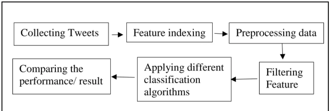
In this paper, we follow some steps to perform sentiment analysis such as collecting Twitter feed, preprocessing tweets, feature indexing, filtering feature, applying different
classification algorithms, and comparing the performance / results. Figure 1 shows the overview of the implementation diagram for the sentiment analysis.
Figure 1. Steps to Perform Sentiment Analysis
The first step includes collecting data from Twitter which can be in different format such as pdf, doc, html, csv, etc. For our paper, we collected data in the .csv format and only collected positive and negative tweets.
The second step includes indexing features. In this process the full text is converted into a vector of words which gives us the conversion results in matrix form.
The third step includes the cleaning of the collected Twitter data, which goes through a series of steps: removing punctuations, HTML, extra space, people name, number and symbol etc. that are not necessary for sentiment analysis.
The fourth step is to filter the features by removing irrelevant features for the
classification task and the vector of words is constructed to improve accuracy, scalability and efficiency for the text classifier.
The fifth step applies different machine learning classifiers to do the sentiment analysis such as such as Naïve Bayes, Support Vector Machine, Maximum Entropy, and Boosting classifier.
The final step is comparing the performances or results. The performance evaluation is done for sentiment analysis by calculating precision, recall, accuracy, and F measure for all classifiers.
Collecting Tweets Feature indexing Preprocessing data
Filtering Feature Applying different classification algorithms Comparing the performance/ result
Since we are using the Streaming API, we have to follow certain steps as listed in the following subsection.
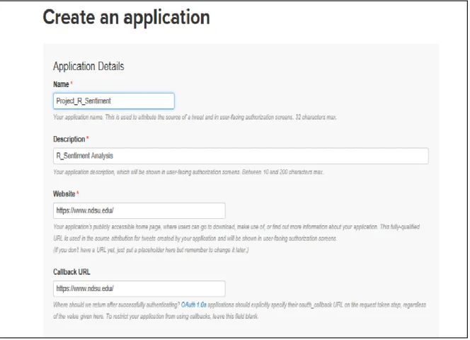
3.2. Creating a New Twitter App
At the beginning, we had to create a Twitter account. Then, we were able to create a new app through Twitter Application Management. Then, we had to fill out the following form (Figure 2):
Figure 2. Create a New Twitter App
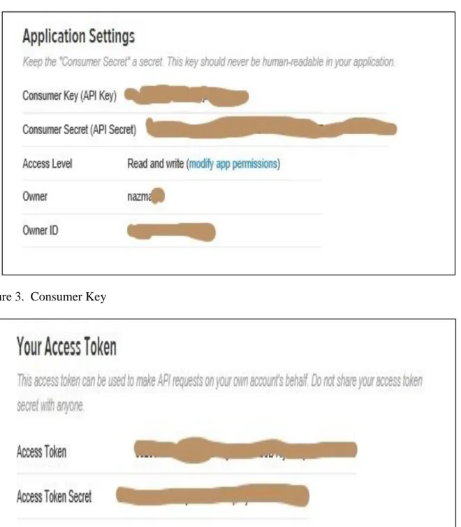
While we are using the Streaming API it allows continuous connection between client and server as long as possible. After creating a new app, when we request a connection from the server it will ask for a key (Figure 3) and access token (Figure 4) that was provided to us from
the Twitter Application manager. After verifying the key and access token through the server we were able to access the streaming connection of Twitter feeds as it occurs.
Figure 3. Consumer Key
3.3. Authorization to Access Twitter in “R”
After getting the key and access token we had to load the Twitter authorization library ‘pacman’ as well as other packages such as ‘twitterR’, ‘ROAuth’, ‘RCurl’. The ‘twitteR’ packages provide a way to interact with the Twitter web API. After providing the login
credentials to the end user, the ‘ROAuth’ package provides a range of client functions to the web servers. The ‘RCurl’ package provides an easier method for general HTTP requests as well as processing those returned results from the requests. We use this command ‘options
(httr_oauth_cache = T)’ to get user browser base authentication.This authorized ‘R’ to access and search Twitter, and this is only necessary to be done once. After the script was authorized, we were able to obtain the text of the tweets.
3.4. Processing Text Twitter Feed in “R”
After collecting the tweets related to the Search keyword “Facebook”, we processed the Twitter feed text before analysis. Because each tweet may contain additional information that is not necessary to perform sentiment analysis such as punctuation, HTML, extra space, people name, number and symbol and thus need to be removed. We need to clean the tweets to get more accurate sentiments from these twitter feeds. In this case, first we use the ‘sapply’ function to create a list or a vector of words in the data which return the result as a matrix, then we use R code to remove the irrelevant content from the tweet. In the cleaning process we remove retweet, people name, punctuation, numbers, HTML, extra spaces and symbols.
Figure 5. Example of Tweet before Cleaning for Facebook
In Figure 5 we can see the retweet, HTML, people name, extra space, numbers, punctuations, symbols.
Figure 6. Example of Tweet after Cleaning for Facebook
From Figure 6 we can see that there is no symbol, punctuations, numbers, HTML, or extra space.
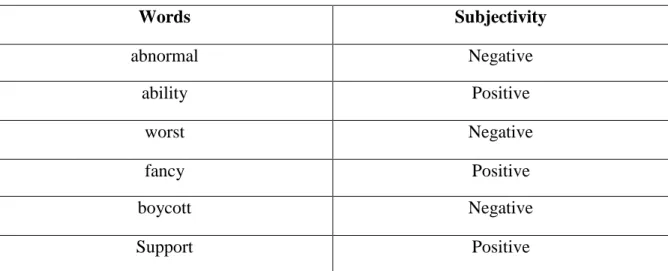
The 'sentiment' package in R has a 'classify_emotion( )' method and we used the method with three arguments. The first argument is the data set to analyze, the second is the
classification algorithm, and the third is a number that specifies to set the prior probability to equal (for Naïve Bayes classifier). The second method we used from the 'sentiment' package was 'classify_polarity( )' trained on Janyce Wiebe’s subjectivity lexicon. This function was provided with two arguments. The first argument was the data set we wanted analyzed, and the second argument is the classification algorithm. There were two options for the classification algorithm for both methods, either the Naïve Bayes classifier or a simple voter procedure. For the
'classify_emotion( )' method, the Naïve Bayes classifier was trained on Carlo Strapparava and Alessandro Valitutti's emotions lexicon. There are six types of emotions widely used in the literature; anger, sadness, joy, disgust, surprise, and fear [14]. For the 'classify_polarity( )' method, the Naïve Bayes classifier was trained on Theresa Wilson, Janyce Wiebe, and Paul Hoffman's subjectivity lexicon. The ‘Classify_polarity( )’ method was use to classify twitter feed into two classes; positive and negative classes. In our experiment, we did not use the neutral class because adding the neutral class could reduce the classifiers’ accuracy [15].
Table 1. Positive and Negative Words from Subjectivity Lexicon
Words Subjectivity abnormal Negative ability Positive worst Negative fancy Positive boycott Negative Support Positive
3.5. Sentiment Analysis with Classifiers
In this paper, we have used four Machine learning algorithms: Naïve Bayes Algorithms, Support Vector Machine, Maximum Entropy algorithms, and Boosting to do sentiment analysis. 3.5.1. Naïve Bayes Classifier
The Naïve Bayes algorithm is a probabilistic classifier based on Bayes’ theorem, which allows to estimate a certain conditional probability for an item with known attributes categorized as a class. It is one of the most well-known supervised classification methods and can be used in text classification. The conditional probability is the probability that the event will occur based on the knowledge of another event having already occurred. The Bayes’ theorem is also related to the term prior probability and posterior probability. The prior probability of an event is the initial probability which is obtained before any additional information is considered. The posterior probability of an event reflects the background knowledge and may use additional information. The Bayes’ Theorem is as follows:
P(A|B) = (1)
In here, we can say that how often A happens given that B happens written as P(A|B), which is the posterior probability. When we know how often B happens given that A happens written P(B|A), which is the likelihood. And how likely A and B are on their own, P(A) and P(B) is the prior probability. In this case, if we consider a hypothesis X to represent A and for an event C to represent B, this can be written as:
P (Ci|X) = (2) P(B) P(B|A) P(A) P(X|Ci) P(Ci) P(X)
Where, P(Ci) is the hypothesis before getting any evidence is the prior probability, P
(Ci|X) is the probability after getting evidence which is posterior probability. And the factor
related is called likelihood ratio. We can restate the Bayes’ theorem as the posterior probability equals to the prior probability times likelihood ratio divided by the predictor
probability [16]. In the above equation, suppose we have class Ci and attributes X. In the Naïve
Bayes’ classifier, we assume that the each specific attribute X= X1, X2,….,Xn for a new item are
conditionally independent of each other given the class. In this case, we do not know to which class it belongs to and our aim is to classify the item. Let the data set be D = {(X1,C1),…, (XN,
CN)}, where N is the number of observations, and n is the number of attributes. So, we can
rewrite the Bayes’ theorem as:
P (Ci| X1, X2, X3,…, Xn) =
(3) Here, we calculate the class probability P(Ci) by counting all possible values of the class variable
C in the data set. And P (X= (X1,X2,X3,…, Xn)|Ci) defines the conditional probability which
includes the joint probability model, that means if X1, X2 and X3 happens then Xn happens. To
classify an item in the data set we calculate P (Ci| X1, X2, X3,…, Xn) for every class C and find the
class with the highest possibility where the item belongs to. If we consider this assumption then the probability of the attributes P(X|Ci) are independent of each other for the given class Ci then
we have the probability of a set of attributes for the given class with the product of the independent probability for every event. We need to maximize
P (X1, X2, X3, ..., Xn|Ci) = P(X1|Ci) × P(X2|Ci) × P(X3|Ci) × … × P(Xn|Ci)
Using this method, we can obtain the frequency in the training data set, within each class for the attribute occurrence.
P(X|Ci)
P(X)
P(X1, X2, X3,…,Xn|C1) +…, + P(X1, X2, X3,…, Xn|CN) P(CN)
In this case we get the conditional probability P(Xi|Ci) by counting:
We can apply the above to the data set as:
P (Ci| X1, X2, X3,…, Xn) =
(4)
With this equation, the probability we get can be used to classify new data without duplicating them.
In this case, we can get the Naïve Bayes classifier as:
CNB = argmax P (C) ∏ P (X|C) (5)
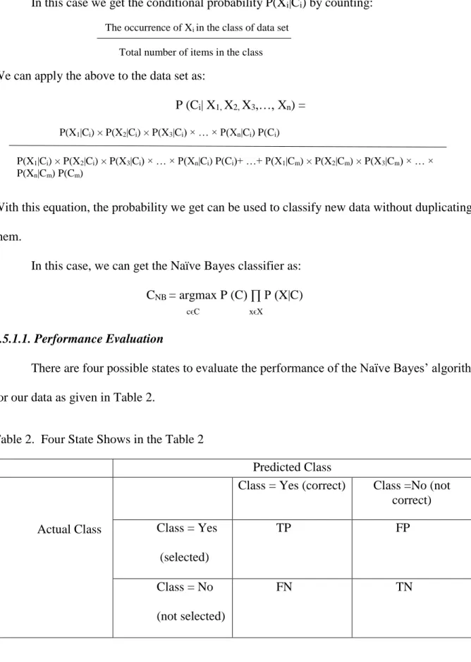
3.5.1.1. Performance Evaluation
There are four possible states to evaluate the performance of the Naïve Bayes’ algorithm for our data as given in Table 2.
Table 2. Four State Shows in the Table 2
Predicted Class
Actual Class
Class = Yes (correct) Class =No (not correct) Class = Yes (selected) TP FP Class = No (not selected) FN TN
The occurrence of Xi in the class of data set
Total number of items in the class
P(X1|Ci) × P(X2|Ci) × P(X3|Ci) × … × P(Xn|Ci) P(Ci)
P(X1|Ci) × P(X2|Ci) × P(X3|Ci) × … × P(Xn|Ci) P(Ci)+ …+ P(X1|Cm) × P(X2|Cm) × P(X3|Cm) × … ×
P(Xn|Cm) P(Cm)
On the above table TP is true positive: if our selected item belongs to the correct class and it is truth then it is called true positive. FN is false negative: in error, if the classifier
indicates that the selected item is not correct, then it is called false negative. FP is false positive: if our classifier incorrectly classifies the item to the correct class then it is called false positive. TN is true negative: if our classifier classifies the item correctly into the not correct class then it is called true negative. With the four states we evaluate each data item in our data set. On one axis the selected data correctly belongs to a class or not, in this case; we call this axis as truth. With the Naïve Bayes’ algorithm, we will identify whether the classifier identifies the correct class the data belongs to.
In our experiment, we use the basic measurement for the evaluation of the performance; which is precision and recall and F measure. We calculate precision and recall and F measure for algorithms Naïve Bayes’, SVM, MaxEnt and Boosting.
Precision: Precision is the ratio (percentage) of the selected item that are correct. Precision = TP/ (TP+FP)
Recall: Recall is the ratio (percentage) of the correct items that we select. Recall = TP/ (TP+FN)
Accuracy: Accuracy is an important measure and is calculated as follows: Accuracy = TP+TN/ (TP+FP+TN+FN)
F-measure: It is a measurement of the test’s accuracy [17]. The F measure is the
weighted average of the precision and recall and the best value for the F measure is in between 1 and 0. This is known as F measure or F score.
2* precision* recall
K-fold Cross Validation: Cross validation is a technique to estimate the predictive model by dividing the original sample data set into training and test sets to train and evaluate the dataset [18]. In the K-fold cross validation method, the original data is randomly divided into K subsets, in every K subsets, 1 subset is assigned for testing, and the remaining k-1 subset are assign for training. We obtain the accuracy from the K times iterations for each K subset, which are averaged over the classifiers.
3.5.2. Support Vector Machine Classifier
Support Vector Machine is a supervised machine learning algorithm which is highly effective for traditional text classification. The basic idea is to find the best line separator that produce a hyperplane that completely separates vectors into non-overlapping classes. The SVM performs a task by constructing a decision surface which maximizes the distance from any data point. The margin of the classifier is determined by this distance from the decision surface to the closest data point. The decision function for an SVM is fully specified by a subset of the data that defines the position of the separator; which is called support vector.
With this algorithm, we plot an individual data item as a point in an n-dimensional space where n is the number of features with its coordinates. Then, we perform classification by
creating the hyperplane which divides two different classes. Suppose we have two objects; one is a circle and other one is a triangle. The hyperplane is the boundary which is separating the two classes. If we want to classify the new object; this will be decided based on the support vector that are the coordinates for the new observation. For SVM we will pick the hyperplane which has the maximum normal distance from any data point as the best separator.
Figure 7. Support Vector Machine for Classification [19]
Support Vector Machine estimates the maximum distance from the data points instead of calculating the probabilities like with the Naïve Bayes classifier.
3.5.3. Maximum Entropy Classifier
The Maximum Entropy Classifier is well suited for text classification problems especially for sentiment analysis. MaxEnt is a probabilistic classifier and belongs to the exponential
classifier category that are based on the principle of Maximum Entropy. According to the principle of Maximum Entropy, when we are estimating the probability distribution, we need to consider the distribution which has the largest entropy. The difference between Naïve Bayes’ is that Naïve Bayes assumes that the features are independent of each other, however, MaxEnt does not assume that the features are independent.
text classification; in text classification all features are words and they are definitely not independent. This classifier uses a search-based optimization technique to find weights for the features to get the maximum likelihood of the training data [21]. At the beginning, this classifier selects a text as a parameter to a random value via search criteria then improves those parameters until it becomes very close to the optimal parameter value. The probability of a specific data point belonging to a specific class can be calculated as follows [21]:
P (c|d, λ) =
(6) In the above equation, c is the class, d is the given data point we are looking for, and the weight is λ. In our project, we want to know the maximum likelihood for each feature without overlapping. With this model, initially it will take a list of words from class c and w for each word, and f (w,c) = N defines a weight joint feature for how many times w happens in a specific class c in a data point. When we are done with calculating this, we will use this equation to estimate the maximum likelihood for the specific class c for the given data point.
3.5.4. Boosting Classifier
The boosting classifier is well suited for classification [22]. The basic idea of the Boosting classifier is to convert a set of weak learners into a strong learner. To convert a weak learner into a strong learner; it takes a family of weak learners first to integrate them and then vote. This way, a family of weak learners turns into a strong learner. Boosting is a machine learning meta algorithm for reducing variance and bias in supervised learning. In Boosting predictive classifiers are used sequentially to build weighted estimates. This classifier takes the weak learning classifier in an iterative way through distribution and adds them into the final
def
∑ exp ∑i λi ƒi (c', d)
c'ϵC
accuracy. The data is re-evaluated after a weak learner is added to the data and the new weight is estimated.
How the Boosting classifier works: To find weak learners, this classifier implements the base learning algorithm with various distributions. The weak learners are sequentially fit on different weighted training data. First, this classifier predicts the original data set and provides equal weight for every observation. For the first learner, if the prediction is not correct, it then provides a higher weighted value to the observation which was predicted incorrectly. This
classifier iteratively produces a new rule every time the base learning algorithm applies to predict a new weak learner. After so many iterations the Boosting classifier reached to the final strong classifier. In our project, by using the Boosting classifier, we want to get accurate predictions by calling weak learners iteratively on different distributions on the training data set.
In this case, it takes a random item as an input from the training data set and applies a decision point to classify that point. After classifying that item, this classifier fits the decision point to finish the training data. This is an iterative process until the complete training data set fits without any error.
4. EXPERIMENTS AND RESULTS 4.1. Dataset
For our experiment, we consider the well-known social media and social networking service company “Facebook” as a keyword to get the data. I searched for 10,000 twitter feeds, and after cleaning the collected Twitter data we had a total of 8,424 tweets for our experiment. In this case, we use the streaming API for capturing tweets, so that we get real time data. We used the same dataset for the testing of the different classifiers, namely Naïve Bayes’, SVM, MaxEnt and Boosting.
4.2. Experiment with Naïve Bayes Classifier
To perform the Naïve Bayes classifier in R, we had to install the e1071 package from the R-CRAN repository archive. David Meyer is the primary developer of this package [24]. This package specifically implements the Naïve Bayes method. Sentiment package was created with more than 6,500 polarity words to determine negative and positive words in the trained dataset. From the trained dataset using the function classify_polarity we can get both positive and negative opinions for Facebook, which is the base to get the results in our project for Naïve Bayes.
4.2.1. Naïve Bayes Performance Evaluation
In our experiment we use precision, recall and accuracy and F-measure to evaluate the Naïve Bayes classifier. From our trained data we got the following rate for precision, recall, accuracy and F measurement.
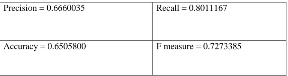
Table 3. Result for Naïve Bayes Classifier
Precision = 0.6660035 Recall = 0.8011167
Accuracy = 0.6505800 F measure = 0.7273385
For this dataset, we got an accuracy rate of 65.05%, which is not a very impressive result. The reason could be that the dataset we used for the Naïve Bayes classifier; where the number of instances might not be large enough, or the attributes that were extracted might have not been very useful. The ratio for recall and F measure is 80.11% and 72.73%, respectively. We are going to compare this result with the other classifiers.
4.3. Experiment with SVM, MaxEnt and Boosting
To do the experiment we had to install RTextTools form the R-CRAN archive. It is a machine learning package in R that allows automatic text classification using different machine learning algorithm [25]. We used the same Facebook dataset that was used for the Naïve Bayes classifier. To perform the experiment with SVM, MaxEnt, and Boosting classifiers; the original dataset was divided into training and testing dataset. 70% of the dataset was used as the training set and 30% was used as the testing set. After cleaning retweets, we had a total of 8,424 data instances left out of 10,000, and we utilized 5,896 (70%) for the training and 2,527 (30%) for the testing.
4.3.1. Support Vector Machine Performance Evaluation
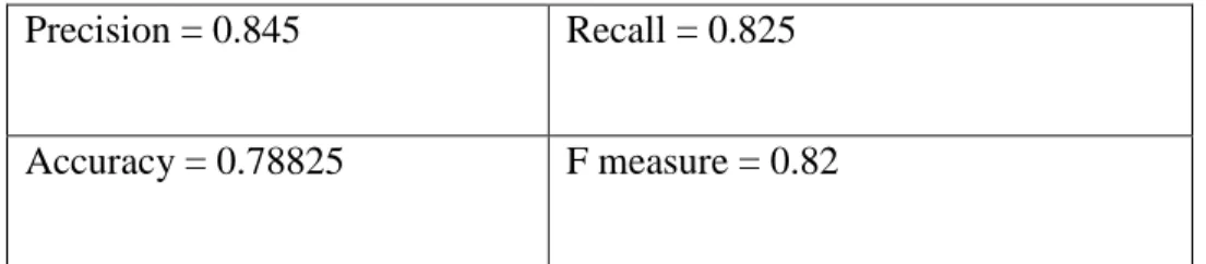
Table 4. Result from Support Vector Machine Precision = 0.845 Recall = 0.825
Accuracy = 0.78825 F measure = 0.82
From Table 4 we can see that the accuracy is 78%, which is an acceptable level and the F measure is 82% which is higher than Naïve Bayes.
4.3.2. MaxEnt Performance Evaluation
We are going to see the result from the MaxEnt Classifier in the Table 5.
Table 5. Result from MaxEnt Classifier Precision = 0.7366667 Recall = 0.88 Accuracy = 0.7649612 F measure = 0.78
We can see that the accuracy rate and F score is still higher than the Naïve Bayes classifier.
4.3.3. Boosting Performance Evaluation
The results from the Boosting algorithm are shown in Table 6.
Table 6. Result from Boosting Classifier
Precision = 0.7966667 Recall = 0.8066667
From the above table we can see that the accuracy is 82% using the Boosting algorithm which is very good for our experiment.
4.3.4. K-Fold Cross Validation
To determine the performance of the model accuracy, we performed K-fold cross validation on the Facebook dataset. It splits the dataset into training and test portions, where 9 datasets are used for training and 1 is used for testing. For the first run, the first fold was used as the first test set, for the second run the second fold was used as the test set, and so on. The result is shown in Figure 9 for Naïve Bayes, Figure 10 for SVM and Figure 11 for MaxEnt and Figure 12 for the Boosting classifier.
4.3.4.1. 10-Fold Cross Validation for Naïve Bayes
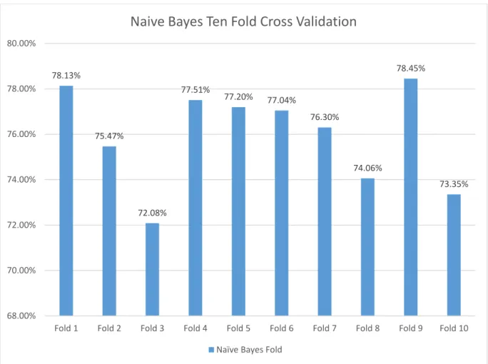
The results we got from 10-fold cross validation using the Naïve Bayes classifier using the Facebook dataset is shown in Figure 9.
Figure 9. 10-Fold Cross Validation for Naïve Bayes Classifier
From the above graph we can see that Fold 9 has the highest performance which is 78.45% for the Naïve Bayes classifier. We can also see that the accuracy varies between 72.08% to 78.45% between the iterations, there are little differences in the data points.
78.13% 75.47% 72.08% 77.51% 77.20% 77.04% 76.30% 74.06% 78.45% 73.35% 68.00% 70.00% 72.00% 74.00% 76.00% 78.00% 80.00%
Fold 1 Fold 2 Fold 3 Fold 4 Fold 5 Fold 6 Fold 7 Fold 8 Fold 9 Fold 10
Naive Bayes Ten Fold Cross Validation
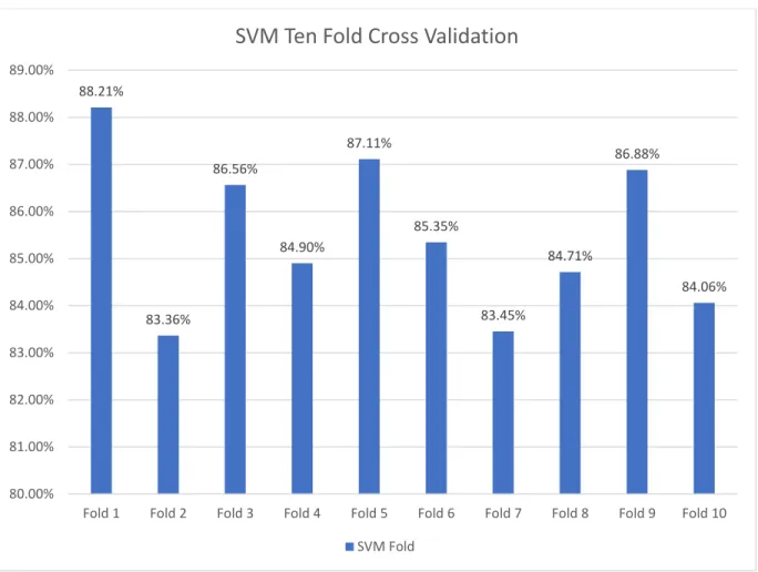
4.3.4.2. 10-Fold Cross Validation for SVM
Figure 10. 10-Fold Cross Validation for SVM Classifier
Figure 10 shows that the highest accuracy we got from the 1st fold and the lowest value we got form the 2nd fold, which is 88.21% and 83.36%.
88.21% 83.36% 86.56% 84.90% 87.11% 85.35% 83.45% 84.71% 86.88% 84.06% 80.00% 81.00% 82.00% 83.00% 84.00% 85.00% 86.00% 87.00% 88.00% 89.00%
Fold 1 Fold 2 Fold 3 Fold 4 Fold 5 Fold 6 Fold 7 Fold 8 Fold 9 Fold 10
SVM Ten Fold Cross Validation
4.3.4.3. 10-Fold Cross Validation for MaxEnt
Figure 11. 10-Fold Cross Validation for MaxEnt classifier
Figure 11 we can see that for the MaxEnt classifier, the highest accuracy rate we got during the 9th fold and the lowest accuracy we got from the 5th fold which is 88.85% and 84.66%, respectively. 87.02% 87.98% 87.08% 87.58% 84.66% 87.32% 87.38% 87.63% 88.85% 86.51% 82.00% 83.00% 84.00% 85.00% 86.00% 87.00% 88.00% 89.00% 90.00%
Fold 1 Fold 2 Fold 3 Fold 4 Fold 5 Fold 6 Fold 7 Fold 8 Fold 9 Fold 10
MaxEnt Ten Fold Cross Validation
4.3.4.4. 10-Fold Cross Validation for Boosting
Figure 12. 10-Fold Cross Validation for Boosting Classifier
Figure 12 shows that the 2nd fold has the highest accuracy, which is 94.76%, and the 9th fold has the lowest accuracy which is 91.11%.
4.3.5. Comparison
To determine the effectiveness and efficiency we need to compare the results among the four classifiers that we used for our experiment. We are going to compare precision, recall, accuracy, and F-measure using K-fold cross validation for Naïve Bayes, SVM, MaxEnt and Boosting classifiers. 91.78% 94.76% 92.87% 91.87% 92.42% 92.60% 91.73% 94.13% 91.11% 91.58% 89.00% 90.00% 91.00% 92.00% 93.00% 94.00% 95.00% 96.00%
Fold 1 Fold 2 Fold 3 Fold 4 Fold 5 Fold 6 Fold 7 Fold 8 Fold 9 Fold 10
Boosting Ten Fold Cross Validation
4.3.5.1. Precision and Recall Comparison
Figure 13. Precision and Recall Comparison for Four Classifiers
We need to calculate precision and recall for the four algorithms that were used for our experiment to get the accuracy. From Figure 13 we can see that SVM has the highest precision and recall percentage, which is 84.50% and 82.50%, respectively, compared to MaxEnt with 73.67% and 88.00%, Boosting with 79.67% and 80.67% and Naïve Bayes with 66.60% and 80.11%. We can say that with the MaxEnt classifier we got the best positive prediction ratio and positive case ratio compared to the other classifiers applied to the Facebook dataset.
4.3.5.2. Accuracy Comparison
The following chart shows the accuracy comparison among the four algorithms; Naïve
66.60% 80.11% 84.50% 82.50% 73.67% 88.00% 79.67% 80.67% 0.00% 10.00% 20.00% 30.00% 40.00% 50.00% 60.00% 70.00% 80.00% 90.00% 100.00% Precision Recall Precision Recall Precision Recall Precision Recall N A ÏV E SV M MA X EN T BO O ST IN G
can evaluate the performance of these classifiers. The value we got by applying the above four algorithms one by one on the original dataset that we obtained using the keyword Facebook.
Figure 14. Sentiment Analysis Accuracy Comparison
Figure 14 shows that Boosting has the highest accuracy value which is 82.18%,
compared to the other three classifiers. This accuracy is used as the percentage for the number of instances of correct positive predictions from all other prediction that were made. Among the four classifiers the accuracy value we obtained are 82.18%, 78.83%, 76.50%, and 65.06% for Boosting, SVM, MaxEnt and Naïve Bayes, respectively.
4.3.5.3. F Measure Comparison for Four Classifiers
Figure 15 shows that SVM has the highest F score which is 83.00% among the four
65.06% 78.83% 76.50% 82.18% 0.00% 10.00% 20.00% 30.00% 40.00% 50.00% 60.00% 70.00% 80.00% 90.00% 100.00%
NAÏVE BAYES SVM MAXENT BOOSTING
77.00%, respectively. F value measures the test’s accuracy. If we get better values for precision and recall, then we will get a better value for the F score. In our experiment, from the F score we can see that SVM, MaxEnt and the Boosting classifier is more effective to perform sentiment analysis on this relatively large dataset than the Naïve Bayes classifier. The reason for the low score for the Naïve Bayes classifier could be that the number of attributes is too little or that the dataset features that were extracted from text was not informational.
Figure 15. F Measure Comparison for Four Classifiers
Figure 13 shows the result for the precision and recall comparison; where we can see that the precision is lower than recall. The reason for this could be that the data may not contain the information that we needed. Otherwise, we can observe the highest percentage of precision and
72.73% 83.00% 78.00% 77.00% 0.00% 10.00% 20.00% 30.00% 40.00% 50.00% 60.00% 70.00% 80.00% 90.00% 100.00%
NAÏVE SVM MAXENT BOOSTING
shows the accuracy for all algorithms. For our dataset we get the highest accuracy when the Boosting classifier is applied which is 82.18%. Figure 15 shows the F measure comparison for all classifiers that was used in this project. It shows that the SVM classifier has the highest ratio which is 83.00%. The F measure is very important to measure the metric base algorithm to determine the effectiveness of the algorithm. From our total dataset we got 5,845 positive tweet which amount to 69.30%, and 2,579 negative tweet which amounts to 30.61%.
5. CONCLUSION AND FUTURE WORK
In this project, our goal was to analyze people opinion on a particular topic by extracting sentiments form Twitter data using different classifiers, i.e. Naïve Bayes, SVM, MaxEnt, and Boosting. After collecting data, we have evaluated the classifier by comparing the accuracy results on the Facebook dataset. To do this, a model was build using “R” (a free software
environment and programming language), and also this model was designed and implemented in the following steps: The first step included collecting data from Twitter which can be in different formats such as pdf, doc, html, csv etc. For our paper we collected data in csv format and only collected positive and negative tweets. The second step included indexing features. During this process the full text is converted into vectors of words which gives us results in matrix form. The third step includes cleaning of the collected Twitter data by going through a series of steps: removing punctuations, HTML, extra space, people name, number and symbol etc. that are not necessary for sentiment analysis. The fourth step filtering feature includes removing irrelevant features and vectors of words are constructed to improve accuracy, scalability and efficiency for the text classifier. The fifth step we applied different machine learning classifiers to do the sentiment analysis such as such as Naïve Bayes, Support Vector Machine, Maximum Entropy and Boosting classifier. The final step is comparing the performance or results. The performance evaluation is done for sentiment analysis by calculating precision, recall, accuracy and F measure for the classifiers. We also performed 10-fold cross validation to evaluate the model accuracy. After comparing all four algorithms we can see that the Boosting classifier has the highest accuracy with 82.18%. Even though Naïve Bayes is said to work best for sentiment analysis, but for our experiment we got better results for the Boosting, SVM and MaxEnt classifiers. Our experimental result shows that Boosting, Support Vector Machine and MaxEnt classifier are
more effective and efficient than the Naïve Bayes algorithm for our chosen real time Twitter data set. From our experiment, we can see that for “Facebook” people have more positive opinion than negative opinion.
As for future research, some research work has been done in the area of Multimodal sentiment analysis. In this research area, L. Morency and his colleagues worked on combination of acoustic, textual and video features to measure opinion polarity in 47 YouTube videos [26]. The basic idea of Multimodal sentiment analysis is not just using traditional text-based sentiment analysis, but it can also include different forms of large data such as images, audio and videos. This type of sentiment analysis holds great promise as an application because it could be really valuable when the traditional textual information is not available [26]. Furthermore, sentiment analysis with Fuzzy logic is another great area to explore in particular for feature-based
sentiment analysis to determine the degree of sentiment. It allows certain degrees of membership which consists of values between 0 and 1.
REFERENCES [1] “Cambridge Core – Twitter as Data” [online]. Available:
https://www.cambridge.org/core/elements/twitter-as-data/27B3DE20C22E12E162BFB173C5EB2592/core-reader. [Accessed 06/19/2018] [2] “Investopedia – Social Networking” [online]. Available:
https://www.investopedia.com/terms/s/social-networking.asp. [Accessed 06/19/2018] [3] B. Liu, "Sentiment Analysis and Subjectivity," in Handbook of Natural Language Processing,
Boca Raton, CRC Press, 2010.
[4] M. Hu and B. Lu, “Mining Opinion Features in Customer Reviews,” in Nineteenth National Conference on artificial Intelligence, San Jose, CA 2004..
[5] B. Liu, “Sentiment Analysis and Opinion Mining, “Morgan & Claypool Publishers, 2012. [6] J. Bollen, H. Mao and X. Zeng, “Twitter Mood Predicts the Stock Market,” in Journal of
computational Science, 2(1), March 2011, Pages 1-8.
[7] J. Smailovic, M. Grcar, N. Lavrac, and M. Znidarsic, “Stream-based Active Learning for Sentiment Analysis in the Financial Domain,” in Journal of ScienceDirect, Information Services, Volume 285, November 2014, Pages 181-203.
[8] X. Ding, B. Liu and P. S. Yu, “A Holistic Lexicon-Based Approach to Opinion Mining,” in WSDM '08, Palo Alto, 2008.
[9] E. Kouloumpis, T. Wilson, and J. Moore, “Twitter Sentiment Analysis: The Good the Bad and the OMG!”, ICWSM, 2011, Pages 538-541.
[10] B. Pang, L. Lee and S. Vaithyanathan, “Thumbs up? Sentiment Classification using Machine Learning Techniques”, EMNLP’02, Volume 10, Pages 79-86.
[11] R. Feldman, “Techniques and Applications for Sentiment Analysis”, Communication of the ACM, Volume 56 Issue 4, 2003, Pages 82-89.
[12] B. Yuan,” Sentiment Analysis of Twitter Data”, Rensselaer Polytechnic Institute, New York, 2016.
[13] P. D. Turney, “Thumbs Up Or Thumbs Down? Sentiment Orientation Applies to
Unsupervised Classification of Reviews”, in Association for Computational Linguistics (ACL), Stroudsburg, 2002, Pages 417-424.
[14] B. Yuan, “Sentiment Analysis of Twitter Data”, Rensselaer Polytechnic Institute, New York, 2016.
[15] H. Li, “Sentiment analysis and opinion mining on Twitter with GMO Keyword”, North Dakota State University, North Dakota, 2016.
[16] “Brilliant – Bayes’ Theorem and Conditional Probability” [online]. Available: https://brilliant.org/wiki/bayes-theorem/. [Accessed 7/17/2018]
[17] A. Yedidia, “Against the F-score” [Online]. Available:
https://adamyedidia.files.wordpress.com/2014/11/f_score.pdf. [Accessed 7/25/2018] WordPress, 2016.
[18] “10-fold Crossvalidation- OpenML” [Online]. Available:
https://www.openml.org/a/estimation-procedures/1. [Accessed 7/28/2018] [19] “Stanford NLP- Support Vector Machines: The linearly separable Case” [Online].
Available: https://nlp.stanford.edu/IR-book/html/htmledition/support-vector-machines-the-linearly-separable-case-1.html. [Accessed 7/20/18].
[20] “DatumBox – Machine Learning Tutorial: The Max Entropy Text Classifier” [Online]. Available: https://blog.datumbox.com/machine-learning-tutorial-the-max-entropy-text-classifier/. [Accessed 7/22/18].
[21] “Christopher Potts, Stanford Linguistics – Sentiment Symposium Tutorial: Classifiers” [Online]. Available: http://sentiment.christopherpotts.net/classifiers.html. [Accessed 7/22/18].
[22] A. Gupte et al., “Comparative Study of Classification Algorithms used in Sentiment Analysis”, in International Journal of Computer Science and Information Technologies, Volume 5 (5), 2014
[23] “Sebastianraschka – Machine Learning FAQ” [Online]. Available:
https://sebastianraschka.com/faq/docs/bagging-boosting-rf.html. [Accessed 7/24/18]. [24] “datascienceplus – Sentiment analysis with machine learning in R” [Online]. Available:
https://datascienceplus.com/sentiment-analysis-with-machine-learning-in-r/. [Accessed 10/13/2018]
[25] “CRAN- Package RTextTools” [Online]. Available:
https://cran.r-project.org/web/packages/RTextTools/index.html. [Accessed 7/28/2018]. [26] E. Cambria, B. Schuller, Y. Xia, C. Havasi, “New Avenues in Opinion Mining and
![Figure 8. Boosting Classifier [23]](https://thumb-us.123doks.com/thumbv2/123dok_us/340838.2537416/30.918.201.674.115.528/figure-boosting-classifier.webp)