Universidade de São Paulo
2015-09
Investigating fitness functions for a
hyper-heuristic evolutionary algorithm in the context
of balanced and imbalanced data classification
Genetic Programming and Evolvable Machines, New York, v. 16, n. 3, p. 241-281, Sep. 2015
http://www.producao.usp.br/handle/BDPI/50993
Downloaded from: Biblioteca Digital da Produção Intelectual - BDPI, Universidade de São Paulo
Biblioteca Digital da Produção Intelectual - BDPI
Investigating fitness functions for a hyper-heuristic
evolutionary algorithm in the context of balanced
and imbalanced data classification
Rodrigo C. Barros•Ma´rcio P. Basgalupp• Andre´ C. P. L. F. de Carvalho
Received: 20 October 2013 / Revised: 21 July 2014 / Published online: 26 October 2014
Springer Science+Business Media New York 2014
Abstract In this paper, we analyse in detail the impact of different strategies to be used as fitness function during the evolutionary cycle of a hyper-heuristic evolu-tionary algorithm that automatically designs decision-tree induction algorithms (HEAD-DT). We divide the experimental scheme into two distinct scenarios: (1) evolving a decision-tree induction algorithm from multiple balanced data sets; and (2) evolving a decision-tree induction algorithm from multiple imbalanced data sets. In each of these scenarios, we analyse the difference in performance of well-known classification performance measures such as accuracy, F-Measure, AUC, recall, and also a lesser-known criterion, namely the relative accuracy improvement. In addition, we analyse different schemes of aggregation, such as simple average, median, and harmonic mean. Finally, we verify whether the best-performing fitness functions are capable of providing HEAD-DT with algorithms more effective than traditional decision-tree induction algorithms like C4.5, CART, and REPTree.
Area Editor for Data Analytics and Knowledge Discovery: Una-May O’Reilly.
Electronic supplementary material The online version of this article (doi:10.1007/s10710-014-9235-z) contains supplementary material, which is available to authorized users.
R. C. Barros (&)
Faculdade de Informa´tica (FACIN), Pontifı´cia Universidade Cato´lica do Rio Grande do Sul (PUCRS), Porto Alegre, Brazil
e-mail: [email protected] M. P. Basgalupp
Instituto de Cieˆncia e Tecnologia (ICT), Universidade Federal de Sa˜o Paulo (UNIFESP), Sa˜o Jose´ dos Campos, Brazil
e-mail: [email protected] A. C. P. L. F. de Carvalho
Instituto de Cieˆncias Matema´ticas e de Computac¸a˜o (ICMC), Universidade de Sa˜o Paulo (USP), Sa˜o Carlos, Brazil
e-mail: [email protected] DOI 10.1007/s10710-014-9235-z
Experimental results indicate that HEAD-DT is a good option for generating algorithms tailored to (im)balanced data, since it outperforms state-of-the-art decision-tree induction algorithms with statistical significance.
Keywords Hyper-heuristicsDecision treesFitness function Imbalanced data
1 Introduction
The automatic design of complex algorithms would benefit researchers from several domains. It was envisioned in the early days of artificial intelligence research, and more recently has been addressed by machine learning and evolutionary compu-tation research groups [29, 34, 38]. The automatic design of machine learning algorithms can be seen as the task of teaching the computer how to create programs that learn from experience.
A recent research area within the combinatorial optimisation field, called hyper-heuristics, has emerged as a suitable tool for the automatic design of algorithms. Hyper-heuristics search in the heuristics space for the most suitable heuristic for a given problem. They can be defined asheuristics to choose heuristics[9].
There are quite few hyper-heuristics that automatically design machine learning algorithms. The pioneering work on that area was the genetic programming-based hyper-heuristic proposed by Pappa and Freitas [29], which evolves complete rule induction algorithms. Sa´ and Pappa [10] proposed an evolutionary algorithm (EA) based hyper-heuristic to automatically design Bayesian Network classifiers, whereas Barros et al. [3] proposed an EA-based hyper-heuristic to automatically design decision-tree induction algorithms called hyper-heuristic evolutionary algorithm for automatically designing decision-tree algorithms (HEAD-DT).
HEAD-DT, which is subject of this paper, is capable of performing quite well when generating a novel decision-tree induction algorithm for a particular problem (data set) [2], and also for a group of data sets [4–6]. Nevertheless, HEAD-DT was employed optimizing always the same objective function (F-Measure), and, moreover, no consistent investigation was performed regarding the ability of HEAD-DT for dealing with data sets that share a particular structural characteristic. Hence, the contribution of this paper is twofold. First, we perform a thorough experimental analysis to verify in detail the impact of different fitness functions during the evolutionary cycle of HEAD-DT. For such, we combine 5 classification performance measures with three aggregation schemes, resulting in 15 different versions of HEAD-DT. Since the classification performance measures are sensitive to the data sets’ level of balance, we investigate separately the 15 versions of HEAD-DT in balanced and imbalanced meta-training sets. Second, after determin-ing the best-performdetermin-ing fitness functions for the balanced and imbalanced data sets, we compare the evolved tree induction algorithm with traditional decision-tree induction algorithms, namely C4.5 [33], CART [7], and REPTree [39].
Our hypothesis is that HEAD-DT is capable of automatically designing decision-tree induction algorithms that are effective in data sets with a particular structural
characteristic. The characteristic here is represented by the balance level of the data sets employed by HEAD-DT. Even though there are many structural characteristics that vary across data sets—noise level, type of attributes, number of classes, just to mention a few—we believe imbalanced-class problems are of crucial importance given that they are found in a large number of domains of great environmental, vital or commercial importance [22].
This paper is organized as follows. Section2 presents a background on hyper-heuristics, whereas Sect.3gives an overview on HEAD-DT. Section4presents the 5 classification performance measures as well as the three aggregation schemes used
during the experiments. Section5 details the methodology we adopted for
conducting the experiments, which are in turn presented in Sect.6. Section7
discusses related work, and Sect.8concludes the paper and points to future research directions.
2 Background on hyper-heuristics
Hyper-heuristics are related to metaheuristics, with the difference that they operate on a search space of heuristics, whereas metaheuristics operate on a search space of solutions to a specific problem. Nevertheless, hyper-heuristics usually employ typical metaheuristics (e.g., evolutionary algorithms) as the search methodology to look for suitable heuristics to a computational problem [31].
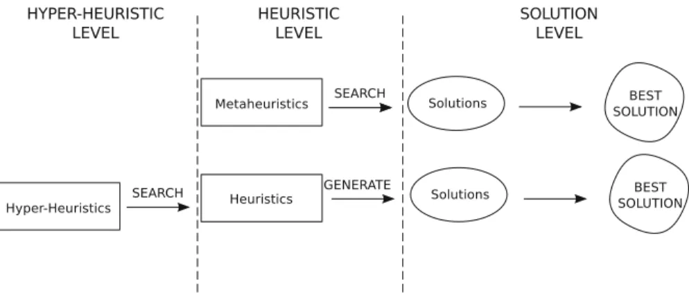
Given that an algorithm or its components can be seen as heuristics, one may see why hyper-heuristics are suitable tools to automatically design custom (tailor-made) algorithms. Figure1 depicts how metaheuristics and hyper-heuristics work at different generality levels. It is possible to see that whereas metaheuristics perform the search in the space of candidate solutions, hyper-heuristics perform the search in the space of candidate heuristics (algorithms), which in turn generate solutions for the problem at hand.
To illustrate that rationale, let us compare two different evolutionary approaches in decision-tree induction for medical data. In the first approach, an evolutionary algorithm is used to evolve the best decision tree for a data set of a particular hospital. In the second approach, an evolutionary algorithm is used to evolve the best decision-tree induction algorithm to be further applied to any given medical data sets. In the first approach, the evolutionary algorithm works as a metaheuristic, because it searches for the best decision tree to the hospital data, and the ultimate goal is to achieve an accurate decision tree for this particular problem. In the second approach, the evolutionary algorithm works as a hyper-heuristic, because it searches for the best decision-tree induction algorithm, which in turn generates decision trees from different instances of medical applications. The second approach is problem independent—instead of generating a decision tree that is only useful for classifying patients from that particular hospital data set, it generates a decision-tree induction algorithm that can be applied to several medical data sets.
Most of the hyper-heuristic research aims at solving typical optimisation problems, such as production scheduling [15,37], educational timetabling [26], 1D packing [24], 2D cutting and packing [18], constraint satisfaction [36], and vehicle
routing [19]. Applications of hyper-heuristics to machine learning are not so frequent and much more recent than optimisation applications. Examples of hyper-heuristic approaches in machine learning include the work of Stanley and Miikkulainen [34], which proposes an evolutionary system for optimising neural network topologies; the work of Oltean [27], which proposes the evolution of evolutionary algorithms through a steady-state linear genetic programming approach; the work of Pappa and Freitas [29], which proposes the evolution of complete rule induction algorithms through grammar-based genetic programming; the work of Vella et al. [38], which proposes the evolution of heuristic rules in order to select distinct split criteria in a decision-tree induction algorithm; and finally the work of Barros et al. [2–4], which propose the evolution of complete decision-tree induction algorithms through a linear-genome evolutionary algorithm, called HEAD-DT. The latter is the object of study in this paper.
3 Overview of HEAD-DT
HEAD-DT [2–4] is a hyper-heuristic evolutionary algorithm capable of automat-ically designing complete top-down decision-tree induction algorithms. Thus, it provides an alternative to the manual design of such algorithms. HEAD-DT can be seen as a regular generational evolutionary algorithm in which individuals are collections of building blocks of top-down decision-tree induction algorithms. HEAD-DT employs typical operators from evolutionary algorithms, such as tournament selection, mutually-exclusive genetic operators (reproduction, cross-over, and mutation), and a typical stopping criterion that halts evolution after a predefined number of generations.
Each individual in HEAD-DT is encoded as an integer vector (see Fig.2), and each gene can take on a value in a predefined range of values. The set of genes is divided in four categories that represent the major types of building blocks (design components) of a top-down decision-tree induction algorithm, namely: split genes, stopping criteria genes, missing value genes, and pruning genes.
3.1 Building blocks
The linear genome that encodes individuals in HEAD-DT holds two genes for the splitcomponent of decision trees. These genes represent the design component that is responsible for selecting the attribute to split the data in the current node of the decision tree. To model this design component, we make use of two different genes. The first one,criterion, is an integer that indexes one of the 15 splitting criteria that are implemented in HEAD-DT. The second gene that controls the split component of a decision-tree algorithm isbinary split. It is a binary gene that indicates whether the splits of a decision tree are going to be binary or multi-way.
The top-down induction of decision trees is recursive and it continues until a stopping criterion (also known aspre-pruning) is satisfied. The linear genome in HEAD-DT holds two genes for representing this design component:criterionand parameter. The first gene, criterion, selects among five different strategies for stopping the tree growth, whereas geneparameterdynamically adjusts a value in the range [0, 100] to the corresponding strategy.
The next design component of decision trees that is represented in the linear genome of HEAD-DT is the missing value treatment. Missing values may be an issue during tree induction and also during classification, and thus we make use of three genes to represent missing values strategies in different moments of the induction/deduction process.
HEAD-DT holds two genes for pruning strategies of top-down decision trees. The first gene, method, indexes one five well-known approaches for pruning a
Fig. 2 Linear-genome for evolving decision-tree
induction algorithms [4]
decision tree, and also the option of not pruning at all. The second gene,parameter, is in the range [0, 100] and its value is again dynamically mapped by a function according to the selected pruning method.
To illustrate one possible individual encoded by HEAD-DT’s linear genome, assume an individual that takes the following values: [4, 1, 2, 77, 3, 91, 2, 5, 1]. Such an individual accounts for Algorithm 1. For a detailed description on HEAD-DT’s building blocks, please refer to [3,4].
Algorithm 1Example of a decision-tree induction algorithm automatically designed by HEAD-DT.
1:Recursively split nodes with the G statistics criterion;
2:Create one edge for each category in a nominal split;
3:Perform step 1 until class-homogeneity or the maximum tree depth of 7 levels ((77 mod 9) + 2) is reached;
4:Perform MEP pruning withm=91; When dealing with missing values:
5:Distribute missing-valued instances to the partition with the largest number of instances;
6:Distribute missing values by assigning the instance to all partitions;
7:For classifying an instance with missing values, explore all branches and combine the results.
3.2 Search space
To compute the search space reached by HEAD-DT, consider the linear genome presented in Fig.2: [split criterion, split type, stopping criterion, stopping parameter, pruning strategy, pruning parameter, mv split, mv distribution, mv classification]. There are 15 types of split criteria, 2 possible split types, 4 types of missing-value strategies during split computation, 7 types of missing-value strategies during training data distribution, and 3 types of missing-value strategies during classification. Hence, there are 152473¼2;520 possible different algorithms.
Now, let us analyse the combination of stopping criteria and their parameters. There is the possibility of splitting until class homogeneity is achieved, and no parameter is needed (thus, 1 possible algorithm). There are 9 possible parameters when the tree is grown until a maximum depth, and 20 when reaching a minimum number of instances. Furthermore, there are 10 possible parameter values when reaching a minimum percentage of instances and 7 when reaching an accuracy threshold. Hence, there are 1þ9þ20þ10þ7¼47 possible algorithms just by varying the stopping criteria component.
Next, let us analyse the combination of pruning methods and their parameters. Reduced-error pruning parameter may take up to 5 different values, whereas pessimistic-error pruning may take up to 4. Minimum-pessimistic-error pruning can take up to 101 values, and error-based pruning up to 50. Finally, cost-complexity pruning takes up to 4 values for its first parameter and up to 5 values for its second. Therefore, there are 5þ4þ101þ ð45Þ þ50¼180 possible algorithms by just varying the pruning component.
If we combine all the previously mentioned values, HEAD-DT currently searches in the space of 2;52047180¼21;319;200 algorithms. Now, just for the sake of argument, suppose a single decision-tree induction algorithm takes about 10 s to produce a decision tree for a given (small) data set for which we want the best possible
algorithm. If we were to try all possible algorithms in a brute-force approach, we would take 59,220 h to find out the best possible configuration for that data set. That means2,467 days or 6.75 years just to find out the best decision-tree algorithm for a single (small) data set. HEAD-DT would take, in the worst case, 100,000 s—10,000 individuals (100 individuals per generation, 100 generations) times 10 s. Thus HEAD-DT would take about 1,666 min (27.7 h) to compute the (near-)optimal algorithm for that same data set, i.e., it is2,138 times faster than the brute-force approach. In practice, this number is much smaller considering that individuals are not re-evaluated if not changed, and HEAD-DT implements reproduction and elitism.
Of course there are no theoretic guarantees that the (near-)optimal algorithm found by HEAD-DT within these 27.7 h is going to be the same global optimal algorithm provided by the brute-force approach after practically 7 years of computation, but its use is justified by the time saved during the process.
3.3 Fitness function
In order to compute the fitness of each individual (candidate decision-tree induction algorithm) during the evolutionary process, HEAD-DT employs ameta-training set. Ameta-test setis used to assess the quality of the evolved algorithm, which is the best individual produced by HEAD-DT. The search for good individuals during evolution can be performed under two distinct frameworks:
• Evolution of a decision-tree algorithm tailored to one specific data set at a time (specific framework);
• Evolution of a decision-tree induction algorithm from multiple data sets (general framework).
Specifically regarding the general framework, HEAD-DT may be executed with distinct goals, namely:
1. Evolving a single decision-tree algorithm for data sets from a particular application domain;
2. Evolving a single ‘‘all-around’’ decision-tree algorithm that is robust in a variety of heterogeneous data sets;
3. Evolving a single decision-tree algorithm for data sets with a particular structural characteristic.
Previous studies showed through empirical evaluation that HEAD-DT is an effective approach for both specific [2,3] and general frameworks. The latter was applied with the goal of evolving a decision-tree algorithm tailored to a particular domain, e.g., flexible-receptor docking data [5], software effort prediction [6], and gene expression data classification [4].
In the general framework, a given individual is mapped into its corresponding decision-tree induction algorithm. Afterwards, each data set that belongs to the
meta-training set is divided into training and validation—typical values are 70 % for training and 30 % for validation [39]. The term ‘‘validation set’’ is used in here instead of ‘‘test set’’ to avoid confusion with the meta-test set, and also due to the fact that we are using the ‘‘knowledge’’ within these sets to reach for a better solution (the same cannot be done with test sets, which are exclusively used for assessing the performance of an algorithm). The fitness function previously employed by HEAD-DT in the general framework was the average F-Measure computed from the decision trees generated for each data set in the meta-training set. Figure3 illustrates the HEAD-DT’s general framework of fitness evaluation.
In this work, we investigate in detail the impact of different fitness functions during the evolutionary cycle of DT’s general framework, as well as HEAD-DT’s performance when it is employed to solve the third goal of the general framework, namely to evolve a single decision-tree induction algorithm for data sets that share a particular structural characteristic. We focus on data sets that vary widely regarding class imbalance.
In the next section, we present a list of interesting candidate fitness functions that take into account a variety of classification evaluation measures and strategies for combining their values obtained for the meta-training set into a single value.
4 Fitness functions 4.1 Performance measures
Performance measures are important tools for assessing the quality of ML algorithms and models. Notwithstanding, several different measures have been
proposed in the specialized literature with the goal of providing better choices in general or for a specific application domain [14].
In the context of HEAD-DT’s fitness function, and given that it evaluates algorithms (individuals) over data sets, it is reasonable to assume that different classification performance measures could be employed to provide a quantitative assessment of algorithmic performance. In this section we present five different performance measures that we have selected for further investigation as HEAD-DT’s fitness function.
4.1.1 Accuracy
Probably the most well-known performance evaluation measure for classification problems, the accuracy of a model is the rate of correctly classified instances:
accuracy¼ tpþtn
tpþtnþfpþfn ð1Þ
where tp (tn) stands for the true positives (true negatives)—instances correctly classified—, andfp(fn) stands for the false positives (false negatives)—instances incorrectly classified.
Even though most classification algorithms are assessed by the accuracy they obtain in a data set, it must be pointed out that accuracy may be a misleading performance measure. For example, suppose we have a data set whose class distribution is very skewed: 90 % of the instances belong to class A and 10 % to class B. A prediction model that always classifies instances as belonging to class A would achieve 90 % of accuracy, even though it never predicts a class-B instance. In this case, assuming that class B is equally important (or even more so) than class A, we would prefer a model with lower accuracy, but which could eventually correctly predict some instances as belonging to the rare class B.
4.1.2 F-Measure
F-Measure is the harmonic mean of precision and recall:
precision¼ tp
tpþfp ð2Þ recall¼ tp
tpþfn ð3Þ fmeasure¼2precisionrecall
precisionþrecall ð4Þ
Although F-Measure is advocated in the machine learning literature as a single measure capable of capturing the effectiveness of a system, it still completely ignores thetn, which can vary freely without affecting the statistic [32].
4.1.3 AUC
The area under the receiver operating characteristic (ROC) curve (AUC) has been increasingly used as a performance evaluation measure in classification problems. The ROC curve is a graphical approach for displaying the trade-off between the true positive rate (tpr =tp/(tp?fn)) and the false positive rate (fpr=fp/(fp?tn)) of a classifier. ROC graphs have properties that make them especially useful for domains with skewed class distribution and unequal classification error osts [13].
To create such a curve, one needs to build a graph in which thetpr is plotted along they axis and the fpr is shown on the x axis. Each point along the curve corresponds to one of the models induced by a given classifier, and different models are built by varying a probabilistic threshold that determines whether an instance should be classified as positive or negative. Figure4 shows the ROC curves for a pair of classifiers,M1 andM2.
A ROC curve is a two-dimensional depiction of a classifier. To compare classifiers we may want to reduce ROC performance to a single scalar value representing the expected performance, which is precisely the AUC. Since the AUC is a portion of the area of the unit square, its value will always be between 0 and 1. However, because random guessing produces the diagonal dashed line between (0, 0) and (1, 1) (see Fig.4), which has an area of 0.5, no realistic classifier should have an AUC value of less than 0.5. The AUC has an important statistical property: it is equivalent to the probability that the classifier will rank a randomly chosen positive instance higher than a randomly chosen negative instance, which makes of the AUC equivalent to the Wilcoxon test of ranks [25].
The machine learning community most often uses the AUC statistic for model comparison, even though this practice has recently been questioned based upon new research that shows that AUC is quite noisy as a performance measure for classification [20] and has some other significant problems in model compari-son [21,23].
4.1.4 Relative accuracy improvement
Originally proposed in [28], the relative accuracy improvement criterion measures the normalized improvement in accuracy of a given model over the data set’s default accuracy (i.e., the accuracy achieved when using the majority class of the training data to classify the unseen data):
RAI¼
AccDefAcc
1DefAcc ; if Acc[DefAcc AccDefAcc DefAcc ; otherwise 8 > > < > > : ð5Þ
In Eq. (5),Accis the accuracy achieved by a given classifier in the corresponding data set, whereas DefAcc is the default accuracy of the same data set. If the improvement in accuracy is positive, i.e., the classifier accuracy is larger than the default accuracy, the improvement is normalized by the maximum possible
improvement over the default accuracy (1DefAcc). Otherwise, the drop in the accuracy is normalized by the maximum possible drop, which is the value of the default accuracy itself. Hence, the relative accuracy improvement RAI returns a
value between -1 (when Acc=0) and 1 (when Acc=1). Any improvement
regarding the default accuracy results in a positive value, whereas any drop results in a negative value. In caseAcc=DefAcc(i.e., no improvement or drop in accuracy is achieved),RAI=0, as it should be.
The disadvantage of the relative accuracy improvement criterion is that it is not suitable for very imbalanced problems—data sets in which the default accuracy is close to 1—, since high accuracy does not properly translate into high performance for these kinds of problems, as previously seen.
4.1.5 Recall
Also known assensitivity(usually in the medical field) ortrue positive rate, recall measures the proportion of actual positives which are correctly identified as such. For example, it may refer to the percentage of sick people who are correctly classified as having the particular disease. In terms of the confusion matrix, recall is given by:
recall¼ tp
tpþfn ð6Þ
Recall is useful for the case of imbalanced data, in which the positive class is the rare class. However, a classifier that always predicts the positive class will achieve a perfect recall, since it does not take into consideration thefpvalues. This problem is alleviated in multi-class problems, in which each class is used in turn as the positive class, and the average of the per-class recall values is taken.
4.2 Aggregation schemes
All classification measures presented in the previous section refer to the performance of a given classifier in a given data set. When evolving an algorithm from multiple data sets, HEAD-DT’s fitness function is measured as the aggregated performance of the individual in each data set that belongs to the meta-training set. We propose the use of three simple strategies for combining the per-data-set performance into a single quantitative value: (1) simple average; (2) median; and (3) harmonic mean.
The simple average (or alternatively the arithmetic average) is computed by simply taking the average of per-data-set values, i.e.,ð1=NÞ PNi¼1pi, for a
meta-training set withNdata sets and a performance measurep. It gives equal importance to the performance achieved in each data set. Moreover, it is best used in situations where there are no extreme outliers and the values are independent of each other.
The median is computed by ordering the performance values from smallest to greatest, and then taking the middle value of the ordered list. If there is an even number of data sets, since there is no single middle value, any of the middle values
N/2 or (N/2)?1 can be used (or alternatively their average). The median is robust to outliers in the data (extremely large or extremely low values that may influence the simple average).
Finally, the harmonic mean is given byðð1=NÞ PNi¼1piÞ
1
. Unlike the simple average, the harmonic mean gives less significance to high-value outliers, providing sometimes a better picture of the average.
5 Experimental setup
In this section, we present the methodology employed for evaluating the novel fitness functions for HEAD-DT that combine the five classification performance measures presented in Sect.4.1 and the three aggregation schemes presented in Sect.4.2as fitness functions of HEAD-DT. There are a total of 15 distinct fitness functions resulting from this analysis: Accuracy?Simple Average (ACC-A),
Accuracy?Median (ACC-M), Accuracy?Harmonic Mean (ACC-H),
AUC?Simple Average (AUC-A), AUC?Median (AUC-M), AUC?Harmonic
Mean (AUC-H), F-Measure?Simple Average (FM-A), F-Measure?Median
(FM-M), F-Measure?Harmonic Mean (FM-H), Relative Accuracy
Improve-ment?Simple Average (RAI-A), Relative Accuracy Improvement?Median
(RAI-M), Relative Accuracy Improvement ? Harmonic Mean (RAI-H),
Recall?Simple Average (TPR-A), Recall?Median (TPR-M), and Recall? Har-monic Mean (TPR-H).
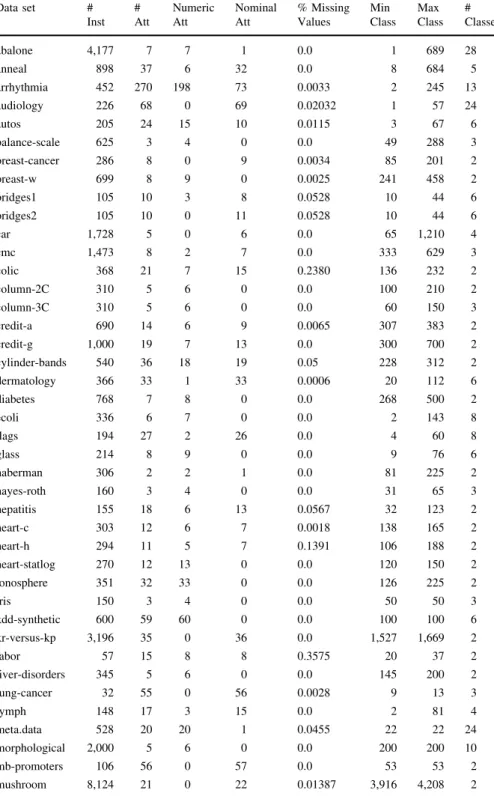
For these experiments, we employed the 67 UCI data sets described in Table1
organized into two scenarios: (1) 5 balanced data sets in the meta-training set; and (2) 5 imbalanced data sets in the meta-training set. These scenarios were created to assess the performance of the 15 distinct fitness functions in balanced and imbalanced data, considering that some of the performance measures are explicitly designed to deal with imbalanced data whereas others are not. The term ‘‘(im)balanced’’ was quantitatively measured according to the imbalance ratio (IR):
IR¼FðADSÞ
FðBDSÞ ð7Þ
whereFðÞreturns the frequency of a given class,ADSis the highest-frequency class
in data setDSandBDS the lowest-frequency class in data setDS.
Regarding the evolutionary parameters of HEAD-DT, we employed typical values found in the literature of evolutionary algorithms for decision-tree induction [1]:
• Population size: 100;
• Maximum number of generations: 100;
• Selection: tournament selection with size t=2;
• Elitism rate: 5 individuals;
• Crossover: uniform crossover with 90 % probability;
Table 1 Summary of the 67 UCI data sets
Data set # # Numeric Nominal % Missing Min Max #
Inst Att Att Att Values Class Class Classes
abalone 4,177 7 7 1 0.0 1 689 28 anneal 898 37 6 32 0.0 8 684 5 arrhythmia 452 270 198 73 0.0033 2 245 13 audiology 226 68 0 69 0.02032 1 57 24 autos 205 24 15 10 0.0115 3 67 6 balance-scale 625 3 4 0 0.0 49 288 3 breast-cancer 286 8 0 9 0.0034 85 201 2 breast-w 699 8 9 0 0.0025 241 458 2 bridges1 105 10 3 8 0.0528 10 44 6 bridges2 105 10 0 11 0.0528 10 44 6 car 1,728 5 0 6 0.0 65 1,210 4 cmc 1,473 8 2 7 0.0 333 629 3 colic 368 21 7 15 0.2380 136 232 2 column-2C 310 5 6 0 0.0 100 210 2 column-3C 310 5 6 0 0.0 60 150 3 credit-a 690 14 6 9 0.0065 307 383 2 credit-g 1,000 19 7 13 0.0 300 700 2 cylinder-bands 540 36 18 19 0.05 228 312 2 dermatology 366 33 1 33 0.0006 20 112 6 diabetes 768 7 8 0 0.0 268 500 2 ecoli 336 6 7 0 0.0 2 143 8 flags 194 27 2 26 0.0 4 60 8 glass 214 8 9 0 0.0 9 76 6 haberman 306 2 2 1 0.0 81 225 2 hayes-roth 160 3 4 0 0.0 31 65 3 hepatitis 155 18 6 13 0.0567 32 123 2 heart-c 303 12 6 7 0.0018 138 165 2 heart-h 294 11 5 7 0.1391 106 188 2 heart-statlog 270 12 13 0 0.0 120 150 2 ionosphere 351 32 33 0 0.0 126 225 2 iris 150 3 4 0 0.0 50 50 3 kdd-synthetic 600 59 60 0 0.0 100 100 6 kr-versus-kp 3,196 35 0 36 0.0 1,527 1,669 2 labor 57 15 8 8 0.3575 20 37 2 liver-disorders 345 5 6 0 0.0 145 200 2 lung-cancer 32 55 0 56 0.0028 9 13 3 lymph 148 17 3 15 0.0 2 81 4 meta.data 528 20 20 1 0.0455 22 22 24 morphological 2,000 5 6 0 0.0 200 200 10 mb-promoters 106 56 0 57 0.0 53 53 2 mushroom 8,124 21 0 22 0.01387 3,916 4,208 2
• Reproduction: cloning individuals with 5 % probability.
Since we compare HEAD-DT with baseline decision-tree induction algorithms C4.5 [33], CART [7], and REPTree [39], we adopted the following procedure for optimising their main parameters: we employed a validation set within the cross-validation procedure (for each set of 9 training folds, we divided it in 75 % for actual training and 25 % for validation), and then selected the optimised pruning parameter of each baseline algorithm for each dataset based on the validation set. For C4.5, the optimised parameter was the confidence factor (CF) that configures its error-based pruning method, varying it within its boundary values [0, 0.5], in steps of 0.05. For CART, the optimised parameter was the number of folds in the cross-validation procedure that is executed within the cost-complexity pruning method (ranging within [2, 20]). For REPTree, the optimised parameter was the size of the
Table 1 continued
Data set # # Numeric Nominal % Missing Min Max #
Inst Att Att Att Values Class Class Classes
postoperative-patient 90 7 0 8 0.0042 2 64 3 primary-tumor 339 16 0 17 0.03904 1 84 21 readings-2 5,456 1 2 0 0.0 328 2,205 4 readings-4 5,456 3 4 0 0.0 328 2,205 4 segment 2,310 17 18 0 0.0 330 330 7 semeion 1,593 264 265 0 0.0 158 1,435 2 sick 3,772 26 6 21 0.0225 231 3,541 2 solar-flare-1 323 11 0 12 0.0 8 88 6 solar-flare-2 1,066 10 0 11 0.0 43 331 6 sonar 208 59 60 0 0.0 97 111 2 soybean 683 34 0 35 0.0978 8 92 19 sponge 76 43 0 44 0.00658 3 70 3 shuttle-control 15 5 0 6 0.2889 6 9 2 tae 151 4 3 2 0.0 49 52 3 tempdiag 120 6 1 6 0.0 50 70 2 tep.fea 3,572 6 7 0 0.0 303 1,733 3 tic-tac-toe 958 8 0 9 0.0 332 626 2 trains 10 25 0 26 0.1154 5 5 2 transfusion 748 3 4 0 0.0 178 570 2 vehicle 846 17 18 0 0.0 199 218 4 vote 435 15 0 16 0.0563 168 267 2 vowel 990 12 10 3 0.0 90 90 11 wine 178 12 13 0 0.0 48 71 3 wine-red 1,599 10 11 0 0.0 10 681 6 wine-white 4,898 10 11 0 0.0 5 2,198 7 zoo 101 16 1 16 0.0 4 41 7
Tabl e 2 Accur acy valu es for the 15 versions of HEAD-DT varyin g the fitness function s ACC ACC ACC A U C A U C AUC FM FM FM RAI RAI RAI TP R T P R TP R AM HA M H A M H A M H A M H ab alone 0.48 0.55 0.50 0.38 0.44 0.34 0.50 0.56 0.50 0.54 0.57 0.53 0.59 0.56 0.50 an neal 1.00 0.99 0.99 0.99 0.99 0.99 0.99 1.00 0.99 1.00 1.00 1.00 1.00 1.00 1.00 arrhy thmi a 0.62 0.61 0.66 0.62 0.63 0.57 0.64 0.60 0.62 0.57 0.64 0.80 0.62 0.59 0.58 au diology 0.85 0.85 0.82 0.78 0.78 0.75 0.82 0.85 0.80 0.85 0.86 0.82 0.84 0.73 0.82 au tos 0.86 0.86 0.86 0.79 0.80 0.79 0.85 0.86 0.86 0.85 0.88 0.87 0.87 0.86 0.84 ba lance-scale 0.85 0.83 0.85 0.84 0.71 0.83 0.85 0.83 0.85 0.86 0.88 0.85 0.87 0.78 0.85 br east-cance r 0.78 0.76 0.77 0.77 0.75 0.76 0.78 0.81 0.77 0.81 0.81 0.78 0.78 0.79 0.77 br east-w 0.97 0.96 0.97 0.96 0.96 0.95 0.97 0.97 0.96 0.96 0.97 0.97 0.97 0.97 0.96 br idges1 0.63 0.75 0.63 0.63 0.69 0.68 0.66 0.74 0.66 0.66 0.73 0.60 0.70 0.77 0.67 br idges2 0.63 0.73 0.59 0.61 0.73 0.65 0.62 0.74 0.61 0.66 0.74 0.61 0.64 0.74 0.64 car 0.95 0.98 0.95 0.94 0.98 0.93 0.95 0.98 0.95 0.95 0.98 0.95 0.96 0.99 0.95 cmc 0.66 0.69 0.66 0.61 0.63 0.60 0.66 0.70 0.66 0.68 0.70 0.67 0.69 0.70 0.66 co lic 0.83 0.85 0.88 0.82 0.83 0.72 0.79 0.83 0.82 0.77 0.88 0.87 0.80 0.80 0.73 co lumn-2 C 0.88 0.90 0.88 0.88 0.89 0.88 0.88 0.89 0.88 0.89 0.89 0.88 0.89 0.90 0.88 co lumn-3 C 0.89 0.87 0.89 0.87 0.87 0.87 0.89 0.89 0.89 0.89 0.89 0.89 0.90 0.87 0.89 cred it-a 0.89 0.88 0.89 0.88 0.89 0.88 0.89 0.90 0.89 0.89 0.90 0.89 0.89 0.89 0.89 cred it-g 0.81 0.81 0.80 0.79 0.81 0.78 0.81 0.84 0.80 0.81 0.84 0.81 0.82 0.82 0.80 cy linder-band s 0.77 0.82 0.82 0.77 0.79 0.73 0.79 0.83 0.80 0.77 0.84 0.83 0.81 0.80 0.71 de rmatol ogy 0.96 0.96 0.96 0.95 0.95 0.95 0.96 0.96 0.96 0.96 0.96 0.96 0.96 0.96 0.96 diab etes 0.83 0.83 0.83 0.81 0.83 0.80 0.83 0.84 0.83 0.84 0.84 0.84 0.85 0.84 0.83 eco li 0.89 0.88 0.89 0.86 0.87 0.86 0.89 0.89 0.89 0.89 0.89 0.89 0.89 0.87 0.89 flags 0.78 0.79 0.76 0.75 0.76 0.74 0.76 0.79 0.76 0.78 0.79 0.78 0.78 0.81 0.76 glass 0.83 0.81 0.83 0.80 0.81 0.79 0.83 0.84 0.83 0.83 0.84 0.83 0.84 0.84 0.84 ha berman 0.79 0.77 0.79 0.78 0.78 0.77 0.80 0.80 0.80 0.80 0.81 0.79 0.81 0.79 0.80
Tabl e 2 cont inued ACC ACC A C C A U C AUC AUC FM FM FM RAI RAI RAI TP R TPR TPR A M H A M H AM HAM HA M H ha yes-roth 0.86 0.86 0.86 0.87 0.87 0.86 0.86 0.87 0.86 0.87 0.87 0.86 0.86 0.87 0.86 he art-c 0.85 0.82 0.85 0.83 0.83 0.82 0.85 0.86 0.85 0.85 0.87 0.85 0.86 0.85 0.85 he art-h 0.84 0.85 0.84 0.84 0.84 0.83 0.81 0.83 0.80 0.85 0.85 0.84 0.79 0.82 0.76 he art-statlog 0.85 0.84 0.85 0.84 0.84 0.84 0.85 0.87 0.85 0.86 0.87 0.85 0.86 0.87 0.85 he patitis 0.87 0.84 0.89 0.87 0.85 0.86 0.88 0.87 0.86 0.85 0.89 0.90 0.85 0.85 0.84 ion osph ere 0.94 0.94 0.94 0.93 0.93 0.93 0.94 0.94 0.94 0.94 0.94 0.94 0.95 0.94 0.94 kdd-sy nth etic 0.93 0.90 0.93 0.90 0.88 0.91 0.93 0.90 0.93 0.93 0.91 0.96 0.93 0.89 0.93 labo r 0.81 0.83 0.81 0.86 0.80 0.80 0.80 0.83 0.79 0.77 0.80 0.87 0.76 0.80 0.73 li ver-disorders 0.79 0.81 0.79 0.77 0.78 0.76 0.79 0.80 0.79 0.80 0.80 0.79 0.82 0.80 0.79 lun g-canc er 0.68 0.58 0.68 0.65 0.68 0.66 0.67 0.70 0.67 0.69 0.71 0.68 0.69 0.66 0.67 lymph 0.85 0.87 0.85 0.83 0.85 0.85 0.85 0.88 0.85 0.86 0.88 0.85 0.85 0.89 0.85 mb -prom oters 0.87 0.86 0.86 0.87 0.87 0.86 0.86 0.89 0.86 0.86 0.89 0.30 0.87 0.88 0.87 met a.data 0.25 0.23 0.30 0.14 0.17 0.10 0.26 0.32 0.29 0.23 0.35 0.87 0.32 0.28 0.23 mo rphologi cal 0.77 0.79 0.78 0.75 0.77 0.75 0.78 0.79 0.78 0.78 0.79 0.78 0.79 0.79 0.78 post operative -patient 0.71 0.72 0.72 0.70 0.70 0.70 0.72 0.73 0.73 0.74 0.73 0.71 0.75 0.72 0.73 pr imary-tu mor 0.51 0.56 0.50 0.47 0.50 0.48 0.47 0.55 0.49 0.53 0.52 0.51 0.54 0.55 0.47 read ings-2 1.00 1.00 1.00 1.00 1.00 1.00 1.00 1.00 1.00 1.00 1.00 1.00 1.00 1.00 1.00 read ings-4 1.00 1.00 1.00 1.00 1.00 1.00 1.00 1.00 1.00 1.00 1.00 1.00 1.00 1.00 1.00 se meion 0.94 0.94 0.94 0.93 0.94 0.93 0.94 0.94 0.94 0.94 0.94 0.97 0.94 0.94 0.94 shut tle-co ntrol 0.66 0.60 0.63 0.59 0.55 0.61 0.63 0.66 0.57 0.63 0.63 0.67 0.63 0.63 0.62 sick 0.99 0.99 0.99 0.99 0.99 0.98 0.99 0.99 0.99 0.98 0.99 0.99 0.99 0.99 0.98 sol ar-flar e-1 0.77 0.77 0.77 0.74 0.76 0.74 0.76 0.78 0.77 0.77 0.78 0.77 0.78 0.78 0.77 sol ar-flar e-2 0.77 0.77 0.77 0.76 0.77 0.76 0.77 0.79 0.77 0.78 0.79 0.77 0.78 0.79 0.77 sonar 0.88 0.84 0.88 0.85 0.84 0.85 0.88 0.87 0.88 0.88 0.87 0.88 0.88 0.83 0.88
Tabl e 2 cont inued ACC ACC ACC AUC AUC AU C F M F M F M RAI RAI RAI TPR TP R T P R AM HA M H A M H A M H A M H soyb ean 0.89 0.87 0.90 0.91 0.88 0.91 0.86 0.90 0.89 0.91 0.88 0.94 0.91 0.89 0.90 spon ge 0.95 0.94 0.95 0.94 0.93 0.93 0.95 0.96 0.95 0.96 0.96 0.95 0.95 0.95 0.95 tae 0.72 0.75 0.72 0.67 0.64 0.67 0.72 0.76 0.72 0.74 0.77 0.72 0.76 0.75 0.73 tem pdiag 1.00 1.00 1.00 1.00 1.00 1.00 1.00 1.00 1.00 1.00 1.00 1.00 1.00 1.00 1.00 tep.fe a 0.65 0.65 0.65 0.65 0.65 0.65 0.65 0.65 0.65 0.65 0.65 0.65 0.65 0.65 0.65 ti c-tac-toe 0.91 0.95 0.90 0.89 0.95 0.89 0.90 0.94 0.90 0.91 0.94 0.91 0.91 0.96 0.91 tra ins 0.87 0.55 0.88 0.78 0.63 0.79 0.77 0.80 0.75 0.88 0.79 0.85 0.67 0.58 0.71 tra nsfusion 0.80 0.79 0.80 0.79 0.79 0.79 0.80 0.81 0.80 0.80 0.81 0.80 0.81 0.80 0.80 ve hicle 0.84 0.86 0.85 0.80 0.82 0.78 0.85 0.86 0.85 0.86 0.86 0.86 0.87 0.85 0.84 vot e 0.97 0.96 0.97 0.97 0.96 0.96 0.96 0.96 0.96 0.97 0.97 0.97 0.96 0.96 0.97 w ine 0.96 0.94 0.96 0.95 0.94 0.95 0.96 0.95 0.96 0.96 0.95 0.96 0.96 0.93 0.96 w ine-red 0.75 0.79 0.77 0.70 0.73 0.67 0.77 0.80 0.77 0.79 0.80 0.78 0.81 0.80 0.76 w ine-white 0.59 0.61 0.59 0.56 0.58 0.55 0.59 0.62 0.59 0.61 0.61 0.78 0.61 0.61 0.58 zo o 0.90 0.91 0.86 0.94 0.95 0.94 0.86 0.96 0.86 0.90 0.91 0.90 0.77 0.96 0.83 A verage rank 8.00 8.93 8.35 11.68 10.7 6 12.5 7 8.25 4.75 9.10 6.41 3 . 72 6.64 4.93 6.88 9.04 Meta-t raining com prises 5 balan ced data sets Bold valu e indicat es the best aver age rank
validation set used in the reduced-error pruning method. The options of values used were: 50 % (1/2 of the training set), 33 % (1/3), 25 % (1/4), 20 % (1/5), 17 % (1/6), 14 % (1/7), 13 % (1/8), 11 % (1/9), and 10 % (1/10). Note that the pruning parameters are the critical parameters that can be set for the baseline decision-tree induction algorithms, so this is why we chose to optimise them.
In order to assess the validity and non-randomness of the obtained results, we present the results of statistical tests by following the approach proposed by Demsˇar [12]. This approach allows the comparison of multiple algorithms on multiple data sets, and it is based on the use of the Friedman test with a corresponding post-hoc test. If the null hypothesis of similar predictive performance is rejected, the Nemenyi post-hoc test for pairwise comparisons is executed. The predictive performance of two classifiers is significantly different if their corresponding average ranks differ by at least the critical difference given by the Nemenyi test.
For better presenting the results of the statistical tests, we employ the graphical representation suggested by Demsˇar [12], the so-called critical diagrams. In this diagram, a horizontal line represents the axis on which we plot the average rank values of the methods. In this axis, the lowest (best) ranks are to the right since we perceive the methods on the right side as the best. When comparing all the algorithms against each other, we connect the groups of algorithms that are not significantly different through a bold horizontal line. We also show the critical difference given by the Nemenyi test on the top of the graph.
6 Experimental results
In this section, we present the results of the two proposed scenarios, namely developing tailor-made decision-tree induction algorithms for balanced (Sect.6.1) and imbalanced data (Sect.6.2). Moreover, we perform a comparison of the best-performing HEAD-DT versions with the baseline decision-tree induction algorithms C4.5, CART, and REPTree, after optimizing their parameters through the previously-described tuning procedure.
6.1 Results for the balanced meta-training set
We randomly selected 5 balanced data sets (IR\1:1) from the 67 UCI data sets described in Table1 to be part of the meta-training set in this experiment: iris (IR=1.0), segment (IR=1.0), vowel (IR =1.0), mushroom (IR=1.07), and kr-versus-kp (IR=1.09).
Tables2and3show the results for the 62 data sets in the meta-test set regarding accuracy and F-Measure, respectively. At the bottom of each table, the average rank is presented for the 15 versions of HEAD-DT created by varying the fitness functions. We did not present standard deviation values due to space limitations within the tables.
By careful inspection of both tables, we can see that their rankings are practically the same, with the median of the relative accuracy improvement being the best-ranked method for either evaluation measure. Only a small position-switching
Tabl e 3 F-Measure values for the 15 versio ns of HEAD -DT var ying the fitness fu nctions ACC ACC ACC A U C A U C AUC FM FM FM RAI RAI RAI TP R T P R TP R AM HA M H A M H A M H A M H ab alone 0.48 0.55 0.50 0.37 0.43 0.33 0.50 0.56 0.50 0.53 0.57 0.53 0.59 0.56 0.49 an neal 0.99 0.99 0.99 0.99 0.99 0.99 0.99 1.00 0.99 1.00 1.00 0.99 1.00 1.00 1.00 arrhy thmi a 0.57 0.56 0.65 0.56 0.58 0.47 0.60 0.53 0.56 0.46 0.62 0.79 0.57 0.52 0.49 au diology 0.84 0.83 0.80 0.75 0.75 0.73 0.81 0.84 0.78 0.84 0.85 0.81 0.83 0.68 0.81 au tos 0.85 0.86 0.86 0.79 0.79 0.78 0.85 0.86 0.86 0.85 0.88 0.87 0.87 0.86 0.84 ba lance-scale 0.85 0.82 0.85 0.82 0.68 0.81 0.85 0.82 0.85 0.87 0.88 0.85 0.87 0.77 0.85 br east-cance r 0.76 0.71 0.72 0.76 0.74 0.75 0.75 0.80 0.74 0.80 0.81 0.76 0.75 0.76 0.73 br east-w 0.97 0.96 0.97 0.96 0.96 0.95 0.97 0.97 0.96 0.96 0.97 0.97 0.97 0.97 0.96 br idges1 0.60 0.74 0.60 0.61 0.69 0.67 0.65 0.73 0.65 0.65 0.73 0.56 0.70 0.77 0.66 br idges2 0.60 0.72 0.54 0.60 0.72 0.64 0.58 0.73 0.57 0.65 0.73 0.56 0.59 0.72 0.60 car 0.95 0.98 0.95 0.94 0.98 0.93 0.95 0.98 0.95 0.95 0.98 0.95 0.96 0.99 0.95 cmc 0.66 0.69 0.65 0.61 0.63 0.60 0.66 0.69 0.66 0.68 0.70 0.66 0.69 0.70 0.66 co lic 0.82 0.85 0.88 0.81 0.82 0.67 0.75 0.82 0.81 0.73 0.88 0.87 0.77 0.77 0.68 co lumn-2 C 0.88 0.90 0.88 0.88 0.89 0.88 0.88 0.89 0.88 0.89 0.89 0.88 0.89 0.90 0.88 co lumn-3 C 0.89 0.87 0.89 0.87 0.87 0.87 0.89 0.89 0.89 0.89 0.89 0.89 0.90 0.86 0.89 cred it-a 0.89 0.88 0.89 0.88 0.89 0.88 0.89 0.90 0.89 0.89 0.90 0.89 0.89 0.89 0.89 cred it-g 0.80 0.78 0.80 0.78 0.81 0.78 0.80 0.84 0.80 0.81 0.84 0.80 0.82 0.79 0.80 cy linder-band s 0.75 0.82 0.82 0.77 0.79 0.72 0.79 0.83 0.80 0.77 0.84 0.83 0.81 0.80 0.69 de rmatol ogy 0.96 0.96 0.96 0.95 0.95 0.95 0.96 0.96 0.96 0.96 0.96 0.96 0.96 0.96 0.96 diab etes 0.83 0.82 0.83 0.81 0.83 0.80 0.83 0.84 0.83 0.84 0.84 0.84 0.85 0.84 0.83 eco li 0.88 0.88 0.88 0.86 0.87 0.86 0.88 0.89 0.88 0.89 0.89 0.88 0.89 0.86 0.88 flags 0.78 0.79 0.76 0.74 0.75 0.74 0.76 0.79 0.76 0.78 0.79 0.78 0.78 0.81 0.76 glass 0.83 0.81 0.83 0.79 0.80 0.78 0.83 0.83 0.83 0.83 0.84 0.83 0.84 0.84 0.84 ha berman 0.78 0.73 0.78 0.76 0.77 0.75 0.78 0.79 0.78 0.79 0.80 0.77 0.80 0.76 0.79
Tabl e 3 cont inued ACC A C C ACC AUC AUC A U C F M F M F M RAI RAI RAI TP R TPR TPR A M H A M H AM HA M H A M H ha yes-roth 0.86 0.86 0.86 0.87 0.87 0.86 0.86 0.86 0.86 0.86 0.87 0.86 0.86 0.86 0.86 he art-c 0.85 0.82 0.85 0.83 0.83 0.82 0.85 0.86 0.85 0.85 0.87 0.85 0.86 0.85 0.85 he art-h 0.84 0.85 0.84 0.84 0.84 0.83 0.79 0.81 0.78 0.85 0.85 0.83 0.75 0.80 0.72 he art-statlog 0.85 0.84 0.85 0.84 0.84 0.84 0.85 0.87 0.85 0.86 0.87 0.85 0.86 0.87 0.85 he patitis 0.85 0.80 0.89 0.86 0.83 0.83 0.86 0.86 0.84 0.82 0.88 0.89 0.83 0.83 0.82 ion osph ere 0.94 0.94 0.94 0.93 0.93 0.93 0.94 0.94 0.94 0.94 0.94 0.94 0.95 0.94 0.94 kdd-sy nth etic 0.93 0.90 0.93 0.90 0.88 0.91 0.93 0.90 0.93 0.93 0.91 0.96 0.93 0.88 0.93 labo r 0.78 0.80 0.79 0.85 0.78 0.77 0.78 0.83 0.76 0.72 0.76 0.87 0.71 0.77 0.67 li ver-disorders 0.79 0.81 0.79 0.77 0.78 0.76 0.79 0.80 0.79 0.80 0.80 0.79 0.82 0.80 0.79 lun g-canc er 0.68 0.54 0.68 0.65 0.68 0.66 0.67 0.70 0.67 0.69 0.71 0.68 0.69 0.64 0.67 lymph 0.85 0.87 0.85 0.83 0.84 0.85 0.85 0.88 0.85 0.86 0.88 0.85 0.85 0.89 0.85 mb -prom oters 0.87 0.86 0.86 0.86 0.87 0.86 0.86 0.89 0.86 0.86 0.89 0.28 0.87 0.88 0.86 met a.data 0.24 0.21 0.28 0.12 0.16 0.08 0.25 0.32 0.28 0.24 0.35 0.86 0.32 0.28 0.23 mo rphologi cal 0.77 0.79 0.77 0.75 0.76 0.74 0.77 0.78 0.77 0.78 0.78 0.78 0.79 0.78 0.78 post operative 0.65 0.66 0.65 0.68 0.66 0.68 0.68 0.72 0.68 0.72 0.72 0.65 0.70 0.69 0.66 pr imary-tu mor 0.48 0.54 0.47 0.43 0.46 0.43 0.44 0.53 0.45 0.50 0.50 0.48 0.51 0.54 0.43 read ings-2 1.00 1.00 1.00 1.00 1.00 1.00 1.00 1.00 1.00 1.00 1.00 1.00 1.00 1.00 1.00 read ings-4 1.00 1.00 1.00 1.00 1.00 1.00 1.00 1.00 1.00 1.00 1.00 1.00 1.00 1.00 1.00 se meion 0.94 0.94 0.94 0.93 0.94 0.93 0.94 0.94 0.94 0.94 0.94 0.97 0.94 0.94 0.94 shut tle-co ntrol 0.63 0.53 0.57 0.52 0.49 0.53 0.58 0.63 0.48 0.58 0.60 0.63 0.56 0.56 0.55 sick 0.99 0.99 0.99 0.99 0.99 0.98 0.99 0.99 0.99 0.98 0.99 0.99 0.99 0.99 0.98 sol ar-flar e-1 0.77 0.76 0.76 0.73 0.75 0.73 0.76 0.77 0.76 0.77 0.77 0.76 0.77 0.77 0.76 sol ar-flar e-2 0.77 0.76 0.76 0.75 0.76 0.75 0.76 0.78 0.76 0.78 0.78 0.77 0.77 0.78 0.76 sonar 0.88 0.84 0.88 0.85 0.84 0.85 0.88 0.87 0.88 0.88 0.87 0.88 0.88 0.83 0.88
Tabl e 3 cont inued ACC ACC ACC AUC AUC AU C F M F M F M RAI RAI RAI TPR TP R T P R AM HA M H A M H A M H A M H soyb ean 0.88 0.85 0.90 0.90 0.87 0.91 0.85 0.89 0.88 0.90 0.87 0.93 0.90 0.87 0.89 spon ge 0.95 0.92 0.94 0.94 0.91 0.92 0.94 0.96 0.94 0.96 0.96 0.95 0.94 0.94 0.93 tae 0.72 0.75 0.72 0.67 0.64 0.67 0.72 0.76 0.72 0.74 0.77 0.72 0.76 0.75 0.73 tem pdiag 1.00 1.00 1.00 1.00 1.00 1.00 1.00 1.00 1.00 1.00 1.00 1.00 1.00 1.00 1.00 tep.fe a 0.61 0.61 0.61 0.61 0.61 0.61 0.61 0.61 0.61 0.61 0.61 0.61 0.61 0.61 0.61 ti c-tac-toe 0.91 0.95 0.90 0.89 0.95 0.89 0.91 0.94 0.90 0.91 0.94 0.91 0.91 0.96 0.91 tra ins 0.87 0.53 0.88 0.78 0.61 0.79 0.77 0.80 0.75 0.88 0.79 0.85 0.66 0.56 0.71 tra nsfusion 0.79 0.75 0.79 0.78 0.78 0.78 0.79 0.80 0.79 0.80 0.80 0.79 0.80 0.77 0.79 ve hicle 0.84 0.86 0.85 0.80 0.82 0.78 0.85 0.86 0.85 0.86 0.86 0.86 0.87 0.85 0.85 vot e 0.97 0.96 0.97 0.97 0.96 0.96 0.96 0.96 0.96 0.97 0.97 0.97 0.96 0.96 0.97 w ine 0.96 0.94 0.96 0.95 0.94 0.95 0.96 0.95 0.96 0.96 0.95 0.96 0.96 0.93 0.96 w ine-red 0.75 0.79 0.77 0.69 0.73 0.66 0.77 0.80 0.77 0.79 0.80 0.78 0.81 0.80 0.76 w ine-white 0.58 0.61 0.59 0.55 0.58 0.53 0.59 0.62 0.59 0.61 0.61 0.78 0.61 0.62 0.58 zo o 0.90 0.90 0.84 0.94 0.95 0.94 0.84 0.96 0.84 0.90 0.91 0.90 0.75 0.96 0.81 A verage rank 7.94 9.22 8.45 11.30 10.5 6 12.3 5 8.17 4.61 9.16 6.27 3 . 60 6.64 5.25 7.17 9.31 Meta-t raining com prises 5 balan ced data sets Bold valu e indicat es the best aver age rank
occurs between the accuracy and F-Measure rankings, with respect to the positions of ACC-M, TPR-H, and FM-H.
Table4summarizes the average rank values obtained by each version of HEAD-DT regarding accuracy and F-Measure. Values in bold indicate the best performing version according to the corresponding evaluation measure. It can be seen that version RAI-M is the best-performing method regardless of the evaluation measure. The average of the average ranks (average across evaluation measures) indicates the following final ranking positions (from best to worst): (1) RAI-M; (2) FM-M; (3) TPR-A; (4) RAI-A; (5) RAI-H; (6) TPR-M; (7) ACC-A; (8) FM-A; (9) ACC-H; (10) ACC-M; (11) FM-H; (12) TPR-H; (13) AUC-M; (14) AUC-A; and (15) AUC-H. The Friedman test provided ap value of 5:151062 for accuracy and 3:78
1058 for F-Measure, indicating that there is a significant difference among the
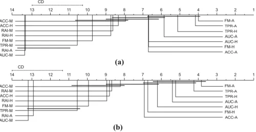
versions of HEAD-DT. For evaluating which differences between versions are statistically significant, we present the critical diagrams of the accuracy and F-Measure values in Fig.5. It is possible to observe that there are no significant differences among the top-4 versions (RAI-M, FM-M, TPR-A, and RAI-A). Nevertheless, RAI-M is the only version that outperforms TPR-M and RAI-H with statistical significance in both evaluation measures, which is not the case of FM-M, TPR-A, and RAI-A.
Some interesting conclusions can be drawn from this first set of experiments with a balanced meta-training set:
• The AUC measure was not particularly effective for evolving decision-tree algorithms in this scenario, regardless of the aggregation scheme being used. It
Table 4 Values are the average performance (rank) of each version of HEAD-DT according to either accuracy or F-Measure
Version Accuracy F-Measure Average
Rank Rank ACC-A 8.00 7.94 7.97 ACC-M 8.93 9.22 9.08 ACC-H 8.35 8.45 8.40 AUC-A 11.68 11.30 11.49 AUC-M 10.76 10.56 10.66 AUC-H 12.57 12.35 12.46 FM-A 8.25 8.17 8.21 FM-M 4.75 4.61 4.68 FM-H 9.10 9.16 9.13 RAI-A 6.41 6.27 6.34 RAI-M 3.72 3.60 3.66 RAI-H 6.64 6.64 6.64 TPR-A 4.93 5.25 5.09 TPR-M 6.88 7.17 7.03 TPR-H 9.04 9.31 9.18
can be seen that versions of HEAD-DT that employ AUC in their fitness function perform quite poorly when compared to the remaining versions—AUC-M, AUC-A, and AUC-H are in the bottom of the ranking: 13th, 14th, and 15th position, respectively;
• The use of the harmonic mean as an aggregation scheme was not successful overall. The harmonic mean was often worst aggregation scheme for the evaluation measures, occupying the lower positions of the ranking (except when combined to RAI).
• The use of the median, on the other hand, was shown to be very effective in most cases. For 3 evaluation measures the median was the best aggregation scheme (relative accuracy improvement, F-Measure, and AUC). In addition, the two best-ranked versions made use of the median as their aggregation scheme;
• The relative accuracy improvement was overall the best evaluation measure, occupying the top part of the ranking (1st, 4th, and 5th best-ranked versions);
• Finally, both F-Measure and recall were consistently among the best versions (2nd, 3rd, 6th, and 8th best-ranked versions), except, once again, when associated with the harmonic mean (11th and 12th).
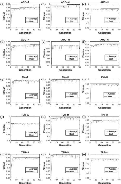
Figure6 depicts a picture of the fitness evolution throughout the evolutionary cycle. It presents both the best fitness from the population at a given generation and the average fitness from the corresponding generation.
The version AUC-M (Fig.6e) achieves the perfect fitness from the very first generation (AUC=1). We further analysed this particular case and verified that the decision-tree algorithm designed in this version does not perform any kind of pruning. Even though prune-free algorithms usually overfit the training data (if no pre-pruning is performed as well, they achieve 100 % of accuracy in the training
(a)
(b)
Fig. 5 Critical diagrams for the balanced meta-training set experiment.aAccuracy rank,bF-Measure rank
0 20 40 60 80 100 0.84 0.86 0.88 0.9 0.92 0.94 0.96 0.98 Generation Fitness ACC−A Average Best (a) 0 20 40 60 80 100 0.93 0.94 0.95 0.96 0.97 0.98 0.99 1 Generation Fitness ACC−M Average Best (b) 0 20 40 60 80 100 0.75 0.8 0.85 0.9 0.95 1 Generation Fitness ACC−H Average Best (c) 0 20 40 60 80 100 0.92 0.93 0.94 0.95 0.96 0.97 0.98 0.99 Generation Fitness AUC−A Average Best (d) 0 20 40 60 80 100 0.97 0.975 0.98 0.985 0.99 0.995 1 1.005 Generation Fitness AUC−M Average Best (e) 0 20 40 60 80 100 0.91 0.92 0.93 0.94 0.95 0.96 0.97 0.98 0.99 Generation Fitness AUC−H Average Best (f) 0 20 40 60 80 100 0.82 0.84 0.86 0.88 0.9 0.92 0.94 0.96 Generation Fitness FM−A Average Best (g) 0 20 40 60 80 100 0.92 0.93 0.94 0.95 0.96 0.97 0.98 0.99 1 Generation Fitness FM−M Average Best (h) 0 20 40 60 80 100 0.75 0.8 0.85 0.9 0.95 1 Generation Fitness FM−H Average Best (i) 0 20 40 60 80 100 0.8 0.85 0.9 0.95 1 Generation Fitness RAI−A Average Best (j) 0 20 40 60 80 100 0.88 0.9 0.92 0.94 0.96 0.98 1 Generation Fitness RAI−M Average Best (k) 0 20 40 60 80 100 0.65 0.7 0.75 0.8 0.85 0.9 0.95 1 Generation Fitness RAI−H Average Best (l) 0 20 40 60 80 100 0.84 0.86 0.88 0.9 0.92 0.94 0.96 0.98 Generation Fitness TPR−A Average Best (m) 0 20 40 60 80 100 0.93 0.94 0.95 0.96 0.97 0.98 0.99 1 Generation Fitness TPR−M Average Best (n) 0 20 40 60 80 100 0.75 0.8 0.85 0.9 0.95 1 Generation Fitness TPR−H Average Best (o)
Tabl e 5 Accur acy valu es for the 15 versions of HEAD-DT varyin g the fitness function s ACC ACC ACC A U C A U C AUC FM FM FM RAI RAI RAI TP R T P R TP R AM HA M H A M H A M H A M H au diology 0.67 0.65 0.69 0.75 0.60 0.60 0.59 0.61 0.60 0.59 0.59 0.55 0.60 0.59 0.60 au tos 0.79 0.74 0.72 0.84 0.63 0.76 0.74 0.49 0.55 0.44 0.47 0.71 0.77 0.35 0.69 ba lance-scale 0.82 0.79 0.81 0.80 0.66 0.69 0.72 0.71 0.71 0.58 0.71 0.80 0.71 0.71 0.71 br east-cance r 0.74 0.73 0.72 0.74 0.60 0.86 0.86 0.70 0.84 0.68 0.84 0.72 0.85 0.62 0.86 br idges1 0.67 0.69 0.66 0.77 0.53 0.87 0.89 0.82 0.84 0.72 0.78 0.68 0.84 0.75 0.84 br idges2 0.64 0.67 0.66 0.73 0.53 0.68 0.70 0.58 0.69 0.55 0.60 0.68 0.67 0.56 0.66 car 0.94 0.92 0.94 0.91 0.76 1.00 1.00 0.94 1.00 0.80 1.00 0.93 1.00 0.94 1.00 he art-c 0.80 0.80 0.80 0.83 0.67 0.76 0.79 0.75 0.76 0.64 0.76 0.80 0.78 0.74 0.79 cmc 0.60 0.58 0.57 0.57 0.50 0.73 0.74 0.60 0.67 0.59 0.66 0.57 0.74 0.59 0.73 co lumn-2 C 0.85 0.84 0.83 0.86 0.69 0.68 0.74 0.61 0.67 0.60 0.66 0.83 0.73 0.56 0.74 co lumn-3 C 0.84 0.84 0.82 0.87 0.70 0.66 0.71 0.50 0.57 0.54 0.59 0.83 0.68 0.47 0.65 cred it-a 0.87 0.88 0.87 0.88 0.70 0.93 0.95 0.83 0.94 0.75 0.91 0.87 0.95 0.77 0.95 cy linder-band s 0.78 0.74 0.72 0.78 0.62 0.77 0.81 0.72 0.76 0.64 0.77 0.73 0.80 0.68 0.82 de rmatol ogy 0.96 0.95 0.93 0.96 0.73 0.86 0.88 0.84 0.87 0.69 0.84 0.92 0.88 0.84 0.88 eco li 0.84 0.85 0.84 0.86 0.68 0.87 0.88 0.85 0.85 0.69 0.84 0.84 0.88 0.84 0.88 flags 0.72 0.68 0.64 0.71 0.56 0.96 0.95 0.92 0.94 0.75 0.91 0.66 0.95 0.92 0.94 cred it-g 0.76 0.75 0.75 0.77 0.63 0.74 0.79 0.70 0.78 0.62 0.73 0.75 0.78 0.70 0.77 glass 0.79 0.79 0.75 0.78 0.62 0.84 0.87 0.77 0.84 0.68 0.80 0.76 0.86 0.71 0.85 ha berman 0.77 0.75 0.75 0.76 0.62 0.85 0.86 0.82 0.86 0.69 0.85 0.76 0.87 0.83 0.87 ha yes-roth 0.85 0.84 0.78 0.85 0.60 0.73 0.77 0.73 0.73 0.61 0.74 0.81 0.76 0.72 0.75 he art-statlog 0.82 0.81 0.80 0.82 0.67 0.93 0.94 0.92 0.95 0.76 0.94 0.80 0.94 0.92 0.93 he patitis 0.81 0.81 0.81 0.89 0.68 0.89 0.86 0.81 0.82 0.66 0.80 0.80 0.86 0.81 0.85 co lic 0.87 0.85 0.85 0.86 0.67 0.79 0.84 0.79 0.84 0.67 0.80 0.86 0.82 0.79 0.82 he art-h 0.82 0.81 0.81 0.82 0.66 0.82 0.85 0.82 0.82 0.68 0.82 0.81 0.84 0.83 0.85
Tabl e 5 cont inued ACC ACC ACC AU C AUC AUC FM FM FM RAI RAI RAI TP R T P R TPR AM HA M H A M H A M H A M H ion osph ere 0.93 0.91 0.91 0.92 0.73 0.79 0.79 0.78 0.78 0.62 0.77 0.92 0.81 0.78 0.80 iris 0.95 0.95 0.95 0.96 0.77 0.82 0.84 0.81 0.82 0.67 0.81 0.95 0.83 0.80 0.84 kr -versus-kp 0.96 0.96 0.96 0.96 0.78 0.73 0.74 0.72 0.72 0.59 0.73 0.96 0.75 0.72 0.74 labo r 0.85 0.77 0.83 0.86 0.68 0.83 0.83 0.79 0.80 0.65 0.80 0.78 0.83 0.79 0.83 li ver-disorders 0.71 0.74 0.71 0.75 0.61 0.83 0.85 0.70 0.83 0.66 0.73 0.73 0.84 0.69 0.80 lun g-canc er 0.62 0.65 0.55 0.65 0.47 0.72 0.74 0.62 0.74 0.58 0.66 0.64 0.74 0.60 0.73 lymph 0.84 0.80 0.80 0.85 0.65 0.85 0.89 0.78 0.83 0.70 0.83 0.79 0.87 0.67 0.89 met a.data 0.13 0.12 0.11 0.10 0.13 0.78 0.83 0.77 0.81 0.66 0.79 0.11 0.82 0.78 0.82 mo rphologi cal 0.74 0.73 0.73 0.73 0.60 0.95 0.96 0.95 0.96 0.77 0.94 0.73 0.97 0.94 0.96 mb -prom oters 0.86 0.85 0.80 0.88 0.63 0.96 0.96 0.95 0.96 0.77 0.95 0.85 0.96 0.96 0.96 mu shroom 0.99 0.98 0.99 0.99 0.80 0.86 0.88 0.85 0.86 0.70 0.86 0.99 0.87 0.82 0.86 diab etes 0.81 0.78 0.78 0.78 0.64 0.87 0.95 0.86 0.95 0.75 0.87 0.78 0.95 0.80 0.95 post operative 0.72 0.71 0.71 0.70 0.57 0.86 0.85 0.79 0.78 0.66 0.78 0.71 0.86 0.77 0.83 se gment 0.96 0.94 0.95 0.94 0.77 0.86 0.90 0.86 0.88 0.71 0.88 0.95 0.90 0.79 0.89 se meion 0.94 0.92 0.93 0.94 0.76 0.10 0.22 0.09 0.13 0.17 0.13 0.93 0.22 0.08 0.18 read ings-2 0.94 0.98 1.00 1.00 0.80 0.92 0.94 0.90 0.93 0.75 0.92 0.95 0.94 0.88 0.94 read ings-4 0.94 0.98 1.00 1.00 0.80 0.92 0.97 0.91 0.96 0.77 0.95 0.95 0.96 0.79 0.97 shut tle-co ntrol 0.60 0.61 0.61 0.57 0.61 0.87 0.98 0.92 0.97 0.78 0.93 0.60 0.98 0.84 0.98 sick 0.97 0.95 0.98 0.98 0.79 0.75 0.79 0.69 0.70 0.58 0.59 0.97 0.81 0.59 0.78 sol ar-flar e-1 0.72 0.73 0.73 0.74 0.60 0.75 0.77 0.75 0.75 0.61 0.75 0.73 0.76 0.74 0.76 sol ar-flar e2 0.76 0.75 0.76 0.75 0.61 0.72 0.76 0.72 0.75 0.60 0.72 0.75 0.77 0.72 0.76 sonar 0.80 0.80 0.79 0.84 0.67 1.00 0.95 1.00 0.94 0.75 0.98 0.80 1.00 1.00 1.00 soyb ean 0.79 0.88 0.83 0.87 0.67 0.58 0.63 0.57 0.62 0.49 0.58 0.68 0.62 0.57 0.62 spon ge 0.93 0.93 0.92 0.95 0.74 0.77 0.83 0.75 0.81 0.65 0.74 0.92 0.83 0.75 0.82
Tabl e 5 cont inued A C C ACC ACC AUC AUC AUC FM FM FM RAI RAI RAI TP R TPR TPR AM HA M H A M H A M H A M H kdd-sy nth etic 0.92 0.92 0.91 0.95 0.74 0.62 0.74 0.62 0.71 0.57 0.64 0.91 0.75 0.60 0.74 tae 0.66 0.62 0.59 0.70 0.53 0.77 0.83 0.74 0.81 0.65 0.72 0.61 0.82 0.69 0.81 tem pdiag 1.00 1.00 0.91 1.00 0.77 0.77 0.81 0.75 0.78 0.64 0.76 0.95 0.81 0.75 0.81 tep.fe a 0.65 0.65 0.65 0.65 0.52 0.81 0.80 0.79 0.82 0.63 0.81 0.65 0.93 0.58 0.90 ti c-tac-toe 0.90 0.88 0.88 0.90 0.73 1.00 0.95 1.00 0.94 0.75 0.98 0.90 1.00 1.00 1.00 tra ins 0.59 0.48 0.37 0.75 0.39 0.65 0.65 0.65 0.65 0.52 0.65 0.51 0.65 0.65 0.65 tra nsfusion 0.77 0.77 0.79 0.79 0.64 0.95 0.94 0.90 0.93 0.74 0.92 0.78 0.95 0.90 0.94 ve hicle 0.79 0.76 0.74 0.76 0.64 0.94 0.96 0.93 0.95 0.76 0.93 0.74 0.96 0.94 0.96 vot e 0.96 0.96 0.96 0.96 0.77 0.98 0.98 0.97 0.98 0.78 0.96 0.96 0.99 0.98 0.98 vow el 0.73 0.75 0.74 0.67 0.62 0.96 0.96 0.95 0.96 0.76 0.95 0.70 0.95 0.95 0.95 w ine 0.93 0.90 0.90 0.96 0.75 0.94 0.99 0.95 0.98 0.78 0.94 0.91 0.99 0.91 0.99 w ine-red 0.69 0.65 0.63 0.62 0.55 0.99 1.00 0.99 1.00 0.80 0.98 0.63 1.00 0.98 1.00 br east-w 0.95 0.94 0.95 0.95 0.76 0.94 0.97 0.95 0.97 0.78 0.95 0.95 0.98 0.95 0.97 zo o 0.94 0.92 0.89 0.93 0.65 0.66 0.82 0.65 0.79 0.61 0.70 0.92 0.88 0.64 0.87 A verage rank 6.70 7.94 8.40 5.87 13.43 6.70 4 . 02 9.71 6.70 13.4 0 8.58 8.72 4.19 10.5 3 5.10 Meta-t raining com prises 5 imbal anced data se ts Bold valu e indicat es the best aver age rank
Tabl e 6 F-Measure values for the 15 versio ns of HEAD -DT var ying the fitness fu nctions ACC ACC ACC A U C A U C AUC FM FM FM RAI RAI RAI TP R T P R TP R AM HA M H A M H A M H A M H au diology 0.63 0.60 0.64 0.71 0.56 0.58 0.54 0.51 0.52 0.52 0.50 0.48 0.48 0.46 0.47 au tos 0.79 0.74 0.71 0.84 0.63 0.76 0.73 0.46 0.54 0.43 0.45 0.71 0.76 0.30 0.68 ba lance-scale 0.81 0.76 0.77 0.78 0.65 0.66 0.67 0.59 0.63 0.53 0.61 0.77 0.60 0.59 0.61 br east-cance r 0.68 0.67 0.68 0.73 0.59 0.86 0.86 0.67 0.84 0.68 0.84 0.65 0.85 0.62 0.86 br idges1 0.62 0.63 0.60 0.77 0.51 0.87 0.89 0.81 0.82 0.71 0.75 0.63 0.83 0.70 0.83 br idges2 0.57 0.60 0.59 0.72 0.50 0.68 0.70 0.58 0.69 0.55 0.60 0.61 0.67 0.56 0.66 car 0.93 0.92 0.94 0.91 0.76 1.00 1.00 0.94 1.00 0.80 1.00 0.93 1.00 0.94 1.00 he art-c 0.80 0.80 0.80 0.83 0.67 0.74 0.78 0.69 0.70 0.62 0.71 0.80 0.76 0.69 0.77 cmc 0.59 0.57 0.57 0.57 0.49 0.73 0.73 0.53 0.61 0.58 0.59 0.57 0.72 0.53 0.71 co lumn-2 C 0.85 0.84 0.83 0.86 0.69 0.67 0.73 0.52 0.62 0.58 0.59 0.83 0.71 0.48 0.72 co lumn-3 C 0.83 0.84 0.82 0.87 0.70 0.66 0.71 0.40 0.53 0.54 0.57 0.82 0.68 0.40 0.65 cred it-a 0.87 0.88 0.87 0.88 0.70 0.93 0.95 0.78 0.94 0.75 0.89 0.87 0.95 0.73 0.95 cy linder-band s 0.78 0.73 0.72 0.78 0.62 0.77 0.81 0.70 0.75 0.63 0.76 0.73 0.80 0.67 0.81 de rmatol ogy 0.96 0.95 0.93 0.96 0.73 0.86 0.88 0.84 0.87 0.69 0.84 0.91 0.88 0.84 0.87 eco li 0.83 0.84 0.83 0.85 0.68 0.87 0.88 0.85 0.84 0.69 0.84 0.83 0.88 0.83 0.88 flags 0.70 0.67 0.62 0.71 0.56 0.96 0.95 0.92 0.94 0.75 0.91 0.63 0.95 0.92 0.94 cred it-g 0.72 0.74 0.72 0.76 0.62 0.74 0.79 0.69 0.78 0.62 0.72 0.73 0.78 0.69 0.77 glass 0.78 0.78 0.74 0.77 0.61 0.84 0.87 0.75 0.84 0.68 0.79 0.74 0.85 0.70 0.85 ha berman 0.71 0.71 0.70 0.75 0.61 0.84 0.86 0.80 0.86 0.68 0.84 0.70 0.86 0.81 0.86 ha yes-roth 0.85 0.83 0.78 0.85 0.59 0.72 0.76 0.68 0.68 0.60 0.70 0.81 0.74 0.68 0.73 he art-statlog 0.82 0.81 0.80 0.82 0.67 0.93 0.93 0.88 0.94 0.75 0.92 0.80 0.93 0.89 0.89 he patitis 0.76 0.75 0.76 0.88 0.66 0.88 0.85 0.76 0.77 0.64 0.76 0.74 0.84 0.76 0.83 co lic 0.87 0.85 0.85 0.86 0.66 0.76 0.83 0.77 0.83 0.67 0.77 0.86 0.80 0.77 0.80 he art-h 0.82 0.80 0.80 0.82 0.66 0.82 0.85 0.82 0.82 0.68 0.82 0.81 0.84 0.83 0.84
Tabl e 6 cont inued ACC ACC ACC AU C AUC AUC FM FM FM RAI RAI RAI TP R T P R TPR AM HA M H A M H A M H A M H ion osph ere 0.93 0.91 0.91 0.92 0.73 0.77 0.78 0.73 0.74 0.62 0.73 0.92 0.78 0.76 0.78 iris 0.95 0.95 0.95 0.96 0.77 0.82 0.84 0.80 0.82 0.67 0.81 0.95 0.83 0.80 0.84 kr -versus-kp 0.96 0.96 0.96 0.96 0.78 0.72 0.73 0.69 0.70 0.58 0.70 0.96 0.73 0.70 0.72 labo r 0.83 0.72 0.83 0.85 0.68 0.83 0.83 0.79 0.80 0.65 0.79 0.74 0.83 0.79 0.83 li ver-disorders 0.69 0.73 0.70 0.75 0.61 0.83 0.85 0.69 0.83 0.66 0.73 0.72 0.84 0.68 0.80 lun g-canc er 0.60 0.64 0.48 0.65 0.42 0.71 0.74 0.59 0.73 0.57 0.64 0.63 0.73 0.56 0.72 lymph 0.83 0.80 0.78 0.85 0.65 0.85 0.89 0.77 0.83 0.70 0.83 0.78 0.87 0.67 0.89 met a.data 0.11 0.10 0.09 0.09 0.12 0.78 0.83 0.77 0.81 0.65 0.78 0.08 0.82 0.77 0.82 mo rphologi cal 0.72 0.71 0.72 0.72 0.60 0.95 0.96 0.95 0.96 0.77 0.94 0.72 0.97 0.94 0.96 mb -prom oters 0.86 0.84 0.80 0.88 0.63 0.96 0.96 0.95 0.96 0.77 0.95 0.85 0.96 0.96 0.96 mu shroom 0.99 0.98 0.99 0.99 0.80 0.86 0.88 0.85 0.86 0.70 0.86 0.99 0.87 0.82 0.86 diab etes 0.80 0.78 0.77 0.78 0.64 0.87 0.95 0.86 0.94 0.75 0.86 0.77 0.95 0.80 0.95 post operative 0.63 0.59 0.59 0.65 0.51 0.86 0.85 0.79 0.78 0.66 0.78 0.59 0.86 0.77 0.83 se gment 0.96 0.94 0.95 0.94 0.77 0.85 0.90 0.86 0.88 0.71 0.88 0.95 0.90 0.78 0.89 se meion 0.94 0.90 0.92 0.93 0.76 0.09 0.21 0.07 0.11 0.16 0.11 0.92 0.21 0.05 0.17 read ings-2 0.93 0.98 1.00 1.00 0.80 0.92 0.94 0.89 0.93 0.75 0.92 0.94 0.94 0.88 0.94 read ings-4 0.93 0.98 1.00 1.00 0.80 0.92 0.97 0.91 0.96 0.77 0.95 0.94 0.96 0.79 0.97 shut tle-co ntrol 0.52 0.49 0.47 0.55 0.52 0.87 0.98 0.92 0.97 0.78 0.92 0.47 0.98 0.83 0.98 sick 0.97 0.94 0.98 0.98 0.79 0.71 0.77 0.63 0.68 0.56 0.54 0.96 0.79 0.51 0.75 sol ar-flar e-1 0.71 0.71 0.71 0.72 0.59 0.74 0.76 0.73 0.73 0.60 0.73 0.70 0.75 0.72 0.74 sol ar-flar e2 0.74 0.73 0.73 0.74 0.60 0.72 0.76 0.70 0.74 0.60 0.72 0.73 0.77 0.69 0.76 sonar 0.80 0.80 0.79 0.84 0.67 1.00 0.93 1.00 0.93 0.74 0.97 0.80 1.00 1.00 1.00 soyb ean 0.77 0.87 0.81 0.86 0.66 0.57 0.63 0.57 0.62 0.49 0.58 0.65 0.62 0.57 0.61 spon ge 0.91 0.91 0.88 0.94 0.73 0.76 0.83 0.74 0.81 0.65 0.74 0.88 0.83 0.74 0.82
Tabl e 6 cont inued A C C ACC ACC AUC AUC AUC FM FM FM RAI RAI RAI TP R TPR TPR AM HA M H A M H A M H A M H kdd-sy nth etic 0.92 0.92 0.91 0.95 0.74 0.61 0.74 0.60 0.71 0.56 0.63 0.91 0.75 0.57 0.73 tae 0.66 0.61 0.59 0.70 0.53 0.76 0.83 0.73 0.81 0.65 0.72 0.61 0.82 0.69 0.80 tem pdiag 1.00 1.00 0.91 1.00 0.77 0.76 0.81 0.71 0.75 0.64 0.75 0.95 0.81 0.73 0.80 tep.fe a 0.61 0.61 0.60 0.61 0.49 0.79 0.78 0.77 0.80 0.61 0.78 0.61 0.93 0.51 0.89 ti c-tac-toe 0.90 0.88 0.88 0.91 0.73 1.00 0.93 1.00 0.93 0.74 0.97 0.90 1.00 1.00 1.00 tra ins 0.59 0.47 0.33 0.75 0.37 0.61 0.61 0.61 0.61 0.49 0.61 0.49 0.61 0.61 0.61 tra nsfusion 0.73 0.71 0.77 0.77 0.63 0.96 0.94 0.90 0.93 0.74 0.92 0.73 0.95 0.90 0.94 ve hicle 0.79 0.75 0.74 0.76 0.64 0.93 0.96 0.92 0.95 0.76 0.92 0.73 0.96 0.94 0.96 vot e 0.96 0.96 0.96 0.96 0.77 0.98 0.98 0.97 0.98 0.78 0.96 0.96 0.99 0.98 0.98 vow el 0.73 0.75 0.74 0.66 0.62 0.96 0.96 0.95 0.96 0.76 0.95 0.69 0.95 0.95 0.95 w ine 0.93 0.90 0.90 0.96 0.75 0.94 0.99 0.95 0.98 0.78 0.94 0.91 0.99 0.91 0.99 w ine-red 0.68 0.63 0.61 0.61 0.54 0.99 1.00 0.99 1.00 0.80 0.98 0.61 1.00 0.98 1.00 br east-w 0.95 0.94 0.95 0.95 0.76 0.94 0.97 0.95 0.97 0.78 0.95 0.95 0.98 0.95 0.97 zo o 0.94 0.91 0.86 0.93 0.62 0.65 0.82 0.65 0.79 0.61 0.69 0.91 0.88 0.64 0.87 A verage rank 6.92 8.23 8.74 5.44 13.23 6.25 3 . 83 9.97 6.79 12.9 4 8.65 8.95 4.27 10.5 6 5.25 Meta-t raining com prises 5 imbal anced data se ts Bold valu e indicat es the best aver age rank
data) and thus underperform in the test data, it seems that this was not the case for the 5 data sets in the training set. In the particular validation sets of the meta-training set, a prune-free algorithm with the stop criterion minimum number of3
instanceswas capable of achieving perfect AUC. Nevertheless, this automatically-designed algorithm probably suffered from overfitting in the meta-test set, since AUC-M was only the 13th-best out of 15 versions.
Versions FM-H (Fig.6i) and TPR-H (Fig.6o) also achieved their best fitness value in the first generation. The harmonic mean, due to its own nature (ignore higher values), seems to make the search for better individuals harder than the other aggregation schemes.
6.2 Results for the imbalanced meta-training set
We randomly selected 5 imbalanced data sets (IR[10) from the 67 UCI data sets described in Table1to be part of the meta-training set in this experiment: primary-tumor (IR=84), anneal (IR=85.5), arrhythmia (IR=122.5), winequality-white (IR=439.6), and abalone (IR=689).
Tables5and6show the results for the 62 data sets in the meta-test set regarding accuracy and F-Measure, respectively. At the bottom of each table, the average rank is presented for the 15 versions of HEAD-DT created by varying the fitness functions. We once again did not present standard deviation values due to space limitations within the tables.
By careful inspection of both tables, we can see that the rankings in them are practically the same, with the average F-Measure being the best-ranked method for either evaluation measure. Only a small position-switching occurs between the accuracy and F-Measure rankings, with respect to the positions of ACC-H and RAI-M.
(a)
(b)
Fig. 7 Critical diagrams for the imbalanced meta-training set experiment.aAccuracy rank,bF-Measure rank
0 20 40 60 80 100 0.53 0.54 0.55 0.56 0.57 0.58 0.59 0.6 0.61 Generation Fitness ACC−A Average Best (a) 0 20 40 60 80 100 0.65 0.7 0.75 0.8 Generation Fitness ACC−M Average Best (b) 0 20 40 60 80 100 0.4 0.42 0.44 0.46 0.48 0.5 Generation Fitness ACC−H Average Best (c) 0 20 40 60 80 100 0.72 0.74 0.76 0.78 0.8 0.82 Generation Fitness AUC−A Average Best (d) 0 20 40 60 80 100 0.7 0.75 0.8 0.85 0.9 0.95 Generation Fitness AUC−M Average Best (e) 0 20 40 60 80 100 0.68 0.7 0.72 0.74 0.76 0.78 0.8 0.82 Generation Fitness AUC−H Average Best (f) 0 20 40 60 80 100 0.48 0.5 0.52 0.54 0.56 0.58 Generation Fitness FM−A Average Best (g) 0 20 40 60 80 100 0.55 0.6 0.65 0.7 0.75 Generation Fitness FM−M Average Best (h) 0 20 40 60 80 100 0.34 0.36 0.38 0.4 0.42 0.44 0.46 Generation Fitness FM−H Average Best (i) 0 20 40 60 80 100 0.24 0.26 0.28 0.3 0.32 0.34 0.36 0.38 Generation Fitness RAI−A Average Best (j) 0 20 40 60 80 100 0.2 0.25 0.3 0.35 0.4 0.45 0.5 Generation Fitness RAI−M Average Best (k) 0 20 40 60 80 100 0.1 0.15 0.2 0.25 Generation Fitness RAI−H Average Best (l) 0 20 40 60 80 100 0.3 0.32 0.34 0.36 0.38 0.4 0.42 Generation Fitness TPR−A Average Best (m) 0 20 40 60 80 100 0.35 0.4 0.45 0.5 0.55 Generation Fitness TPR−M Average Best (n) 0 20 40 60 80 100 0.18 0.2 0.22 0.24 0.26 0.28 0.3 Generation Fitness TPR−H Average Best (o)
Table7summarizes the average rank values obtained by each version of HEAD-DT with respect to accuracy and F-Measure. Values in bold indicate the best performing version according to the corresponding evaluation measure. The version FM-A is the best-performing method regardless of the evaluation measure. The average of the average ranks (average across evaluation measures) indicates the following final ranking positions (from best to worst): (1) FM-A; (2) TPR-A; (3) TPR-H; (4) AUC-A; (5) AUC-H; (6) FM-H; (7) ACC-A; (8) ACC-M; (9) ACC-H; (10) RAI-M; (11) RAI-H; (12) FM-M; (13) TPR-M; (14) RAI-A; and (15) AUC-M. The Friedman test provided ap value of 1:161090 for accuracy and 2:22
1088 for F-Measure, indicating that there is a significant difference among the
versions of HEAD-DT. For evaluating which differences between versions are statistically significant, we present the critical diagrams of the accuracy and F-Measure values in Fig.7. We can see that there are no statistically significant differences among the 7 (5) best-ranked versions regarding accuracy (F-Measure). In addition, It can be observed that the 6 best-ranked versions involve performance measures that are suitable for evaluating imbalanced problems (F-Measure, recall, and AUC), which is actually expected given the composition of the meta-training set.
The following conclusions can be drawn from this second set of experiments concerning imbalanced data sets:
• The relative accuracy improvement is not suitable for dealing with imbalanced data sets and hence occupies the bottom positions of the ranking (10th, 11th, and 14th positions). This behavior is expected given that RAI measures the improvement over the majority-class accuracy, and this improvement is often damaging for imbalanced problems, in which the goal is to improve the accuracy of the less-frequent class(es);
• The median was the worst aggregation scheme overall, figuring in the bottom positions of the ranking (8th, 10th, 12th, 13th, and 15th). It is interesting to
(a)
(b)
Fig. 9 Critical diagrams for accuracy and F-Measure. Values are regarding the 20 UCI data sets in
notice that the median was very successful in the balanced meta-training experiment, and quite the opposite in the imbalanced one;
• The simple average, on the other hand, presented itself as the best aggregation scheme for the imbalanced data, figuring in the top of the ranking (1st, 2nd, 4th, 7th), except when associated with RAI (14th), which was the worst performance measure overall;
• The 6 best-ranked versions were those employing performance measures known to be suitable for imbalanced data (F-Measure, recall, and AUC);
• Finally, the harmonic mean had a solid performance throughout this experiment, differently from its performance in the balanced meta-training experiment.
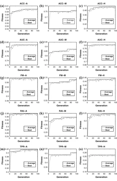
Figure8 depicts a picture of the fitness evolution throughout the evolutionary cycle. According to these results, whereas some versions find their best individual at the very end of evolution (e.g., FM-H, Fig.8i), others converge quite early (e.g., TPR-H, Fig.8o), though there seems to exist no direct relation between early (or late) convergence and predictive performance.
6.3 Experiments with the best-performing fitness functions
Considering that the median of the relative accuracy improvement (RAI-M) was the best-ranked fitness function for the balanced meta-training set, and that the average F-Measure (FM-A) was the best-ranked fitness function for the imbalanced
meta-Table 7 Values are the average performance (rank) of each version of HEAD-DT according to either accuracy or F-Measure
Version Accuracy F-Measure Average
Rank Rank ACC-A 6.70 6.92 6.81 ACC-M 7.94 8.23 8.09 ACC-H 8.40 8.74 8.57 AUC-A 5.87 5.44 5.66 AUC-M 13.43 13.23 13.33 AUC-H 6.70 6.25 6.48 FM-A 4.02 3.83 3.93 FM-M 9.71 9.97 9.84 FM-H 6.70 6.79 6.75 RAI-A 13.40 12.94 13.17 RAI-M 8.58 8.65 8.62 RAI-H 8.72 8.95 8.84 TPR-A 4.19 4.27 4.23 TPR-M 10.53 10.56 10.55 TPR-H 5.10 5.25 5.18
![Fig. 2 Linear-genome for evolving decision-tree induction algorithms [4]](https://thumb-us.123doks.com/thumbv2/123dok_us/338451.2537136/6.659.124.579.76.442/fig-linear-genome-evolving-decision-tree-induction-algorithms.webp)
![Fig. 4 ROC curves for two different classifiers [35]](https://thumb-us.123doks.com/thumbv2/123dok_us/338451.2537136/9.659.137.526.86.401/fig-roc-curves-different-classifiers.webp)