Conditional anomaly detection methods for patient management alert systems

(1)

for patient–management alert systems

Keywords: anomaly detection, alert systems, monitoring, health–care applications, metric learning

Michal Valko _{[email protected]}

Gregory Cooper _{[email protected]}

Amy Seybert _{[email protected]}

Shyam Visweswaran _{[email protected]}

Melissa Saul _{[email protected]}

Milos Hauskrecht _{[email protected]}

Computer Science Department, Department of Biomedical Informatics, University of Pittsburgh, PA, USA Department of Pharmacy and Therapeutics, University of Pittsburgh Medical Center, PA, USA

Abstract

Anomaly detection methods can be very use-ful in identifying unusual or interesting pat-terns in data. A recently proposed condi-tional anomaly detection framework extends anomaly detection to the problem of identi-fying anomalous patterns on a subset of at-tributes in the data. The anomaly always depends (is conditioned) on the value of re-maining attributes. The work presented in this paper focuses on instance–based meth-ods for detecting conditional anomalies. The methods rely on the distance metric to iden-tify examples in the dataset that are most critical for detecting the anomaly. We in-vestigate various metrics and metric learn-ing methods to optimize the performance of the instance–based anomaly detection meth-ods. We show the benefits of the instance– based methods on two real–world detection problems: detection of unusual admission decisions for patients with the community– acquired pneumonia and detection of unusual orders of an HPF4 test that is used to confirm Heparin induced thrombocytopenia — a life– threatening condition caused by the Heparin therapy.

1. Introduction

Anomaly detection methods can be very useful in identifying interesting or concerning events. Typical anomaly detection attempts to identify unusual data instances that deviate from the majority of examples in the dataset. Such instances indicate anomalous (out of ordinary) circumstances, for example, a network at-tack (Eskin, 2000) or a disease outbreak (Wong et al., 2003). In this work, we study conditional anomaly de-tection (Hauskrecht et al., 2007) framework that ex-tends standard anomaly detection by identifying par-tial patterns in data instances that are anomalous with respect to the remaining data features. Such a frame-work is particularly promising for identifying unusual patient–management decisions or patient outcomes in clinical environment (Hauskrecht et al., 2007). Our conditional anomaly detection approach is in-spired by classification model learning. Let x defines a vector of input attributes (representing the patients state) andydefines the output attribute (representing the target patient–management decision). Our goal is to decide if the example (x, y) is conditionally anoma-lous with respect to past examples (patients) in the database. In other words, we ask if the patient man-agement decisionyis unusual for the patient condition x, by taking into account records for past patients in the database. Our anomaly detection framework works by first building a discriminative measure d(·) that reflects the severity with which an example dif-fers from conditional (input–to–output) patterns ob-served in the database. All anomaly calls are then de-fined relative to this measure. To constructdwe rely on methods derived from classification model learning.

(2)

In particular, our method exploits discriminant func-tions often used to make classification model calls. We investigate and experiment with discriminative mea-sures derived from two classification models: the Na¨ıve Bayes model (Domingos & Pazzani, 1997) and the sup-port vector machines (Vapnik, 1995).

The anomaly detection call for the current instance (patient) can be made with respect to either all pa-tients in the database or their smaller subset. In this work we pursue instance–based anomaly detection ap-proach. The instance–based methods do not try to learn a universal predictive model for all possible pa-tient instances at the same time, instead the model is optimized for every data instance (patient) individu-ally. The instance–specific model Mx may provide a

better option if the predictive model is less complex and the dataset is small (Aha et al., 1991).

An instance–specific methods typically rely on a dis-tance metric to pick the examples most relevant for the comparison. However, standard distance metrics such as Euclidean or Mahalanobis metrics are not the best for the anomaly detection task since they may be biased by feature duplicates or features that are irrel-evant for predicting the outcome y. Thus, instead of choosing one of the standard distance metrics we in-vestigate and test metric–learning methods that let us adapt predictive models to specifics of the currently evaluated example x.

We investigate two metric–learning methods that were originally used for building non–parametric classifica-tion models. The first method is NCA (Goldberger et al., 2004). The method adjusts the parameters of the generalized distance metric so that the accuracy of the associated nearest neighbor classifier is optimized. The second method, RCA (Bar-Hillel et al., 2005) op-timizes mutual information between the distribution in the original and the transformed space with restric-tion that distances between same class cases do not ex-ceed a fixed threshold. We test the methods and show their benefits on two real–world problems: identifica-tion of unusual patient management decisions for (1) patients suffering from the community acquired pneu-monia, and (2) post–surgical cardiac patients on the Heparin therapy.

2. Methodology

2.1. Conditional anomaly detection

The objective of standard anomaly detection is to iden-tify a data exampleathat deviates from all other ex-amplesEin the database. Conditional anomaly detec-tion (Hauskrecht et al., 2007) is different. The goal is

to detect an unusual pattern relating input attributes xand output attributesyin the examplea, that devi-ates from patterns observed in other examples in the database. To assess the conditional anomaly ofa we propose to first build (learn) a one–dimensional pro-jectiond(·) of the data that reflects the prevailing (or expected) conditional pattern in the database for y given x. The projection model dis then used to an-alyze the deviations of a’s to determine the anomaly. We say that the case a is anomalous in the output attribute(s) y with respect to input x, if the value d(y|x) falls below certain threshold. Our conditional anomaly detection framework can be used for a num-ber of purposes. Our objective here is to use it de-tect anomalous patient–management decisions. In this case the input attributes x define the patients condi-tion and the output attribute y corresponds to the patient–management decision we want to evaluate. 2.2. Discriminative projections

In our work we consider two methods for building discriminative projections d(·). Both of these meth-ods are derived from the models used frequently in classification model learning: the Na¨ıve Bayes model (Domingos & Pazzani, 1997) and the support vector machines (SVM) (Vapnik, 1995). The fact that we use classification models is not a coincidence. Classifica-tion models attempt to learn condiClassifica-tional patterns in between inputs x and class outputs y from the past data and apply them to predict the class membership for the future inputs. In our case, we aim to model the relation between input x and output patterns y and apply it to detect pattern deviations in the new example (x, y). In both cases the model learning at-tempts to capture the prevailing conditional patterns observed in the dataset and the difference is in how the learned patterns are used in the two frameworks. 2.2.1. Na¨ıve Bayes model

A Na¨ıve Bayes classifier (Heckerman, 1995) is a gen-erative classification model used frequently in ma-chine learning literature and comes with excellent dis-criminative performance on many ML datasets. The Na¨ıve Bayes model is a special Bayesian belief network (Pearl, 1988; Lauritzen & Spiegelhalter, 1988) that de-fines the full joint probability of variables x and the class variabley as:

P(x, y) =P(y)P(x|y) =P(y) k

Y

i=1

P(xi|y)

(3)

pa-rameters: (1) prior distribution on class variable and (2) class–conditional densities for all featuresx. This decomposition reflects the major assumption behind the model: all features (attributes) of x are indepen-dent given the class variableywe would like to predict. We note that any probabilistic calculation can be per-formed once the full joint model is known. The param-eters of the Na¨ıve Bayes model can be learned using the maximum likelihood or the Bayesian approaches from the training data. We adopt the Bayesian frame-work to learn the parameters of the model and com-pute any related statistics. Let M define the Na¨ıve Bayes model. In such a case the parametersθM of the model M are treated as random variables and are de-scribed in terms of a density function P(θM|M). To simplify the calculations we assume (Heckerman, 1995) (1) parameter independence and (2) conjugate priors. In such a case, the posterior follows the same distribu-tion as the prior and updating reduces to updates of sufficient statistics. Similarly, many probabilistic cal-culations can be performed in the closed form. The Na¨ıve Bayes model predicts the classy by calculating the class posterior P(y|x). If one model is used then the class posterior is calculated as:

P(y|x) = P(y)P(x|y) P(x) ∝P(y) k Y i=1 P(xi|y)

The Na¨ıve Bayes model can be adopted for the anomaly detection purposes by defining the discrim-inative projection of an example (x, y) to be equal to the class posterior, that is: d(y|x) = P(y|x). In this case the projection has an intuitive probabilistic in-terpretation: an example (x, y) is anomalous if the probability of the decision y with respect to its in-put attributes x and past examples in the database is small. Moreover, the smaller is the probability, the more likely is the anomaly. We note that the Na¨ıve Bayes model described here can easily extend to more complex generative models based on the Bayesian be-lief networks.

2.2.2. Support vector machines

The support vector machine (SVM) (Vapnik, 1995; Burges, 1998) is a discriminative machine learning model very popular in the machine learning commu-nity primarily thanks to its ability to learn high– quality discriminative patterns in high–dimensional datasets. In our work we adopt the linear support vector machine algorithm to build the conditional pro-jectiondfor the anomaly detection purposes.

The linear support vector machine learns a linear decision boundary that separates the n–dimensional

feature space into 2 partitions corresponding to two classes of examples. The boundary is a hyperplane given by the equation

wTx+w0= 0,

where w is the normal to the hyperplane, and w0 is the distance separating the “support vectors” — a set of representative training examples from each class which are most helpful for defining the decision boundary. The parameters of the model (w and w0) can be learned from the data through quadratic opti-mization using a set of Lagrange parameters (Vapnik, 1995). These parameters allow us to redefine the de-cision boundary as wTx+w0= X i∈SV ˆ αiyi(xTix) +w0,

where only samples in the support vector set (SV) con-tribute to the computation of the decision boundary. To support classification tasks, the projection defining the decision boundary is used to determine the class of a new example. That is, if the value

wTx+w0≥0

is positive then C(x) belong to one class, if it is neg-ative it belongs to the other class. However, in our conditional anomaly framework we use the projection itself for the positive class and the negated projection for the negative class to measure the deviation:

d(y|x) =y(wTx+w0), wherey∈ {−1,1} In other words, the smaller the projection is the more likely is the example anomalous. We note that the negative projections correspond to misclassified exam-ples.

2.3. Instance–specific models

Discriminative models used for anomaly detection pur-poses can be of different complexity. However, if the dataset used to learn the model is relatively small, a more complex model may become very hard to learn reliably. In such a case a simpler parametric model with a smaller number of parameters may be pre-ferred. Unfortunately, a simpler model may sacrifice some flexibility and its predictions may become biased towards the population of examples that occurs with a higher prior probability. To make more accurate pre-dictions for any instance, we resort toinstance–specific predictive methods and models (Aha et al., 1991). The models in instance–based methods are individually op-timized for every data instance x. To reflect this, we

(4)

denote the predictive model forxas Mx. The benefit

of the instance–based models is its more accurate fit to any data instance; the limitation is that the models must be trained only on the data that are relevant for x. Choosing the examples that are most relevant for training the instance–specific model is the bottleneck of the method. We discuss methods to achieve this later on.

3. Selecting relevant examples

3.1. Exact match.

Clearly, the best examples are the ones that exactly match the input attributes of the instancex. However, it is very likely that in real–world databases none or only few cases match the target case exactly so there is no or a very weak population support to draw any statistically sound anomaly conclusion.

3.2. Similarity–based match

One way to address the problem of insufficient popu-lation available through the exact match is to define a distance metric on the space of attributes C(x) that lets us select the examples closest to the target ex-amplex. The distance metric defines the proximity of any two cases in the dataset, and thekclosest matches to the target case define the best population of sizek. Different distance metrics are possible. An example is the generalized distance metricr2 _defined:

r2(xi,xj) = (xi−xj)TΓ−1(xi−xj), (1) where Γ−1 is a matrix that weights attributes of pa-tient cases proportionally to their importance. Differ-ent weights lead to a differDiffer-ent distance metric. For example, if Γ is the identity matrixI, the equation de-fines the Euclidean distance of xi _{relative to}_xj_{. The} Mahalanobis distance (Mahalanobis, 1936) is obtained from (1) by choosing Γ to be the population covariance matrix Σ which lets us incorporate the dependencies among the attributes.

The Euclidean and Mahalanobis metrics are standard off–shelf distance metrics often applied in many learn-ing tasks. However, they come with many deficiencies. The Euclidean metric ignores feature correlates which leads to “double–counting” when defining the distance in between the points. The Mahalanobis distance re-solves this problem by reweighting the attributes ac-cording to their covariances. Nevertheless, the major deficiency of both Mahalanobis and Euclidean metrics is that they may not properly determine the relevance of an attribute for predicting the outcome attributey. The relevance of input attributes for anomaly

detec-tion is determined by their influence on the output attribute y. Intuitively, an input attribute is relevant for the outputyif is able to predict or help to predict its changes. To incorporate the relevance aspect of the problem into the metric we adapt (learn) the param-eters of the generalized distance metric with the help of examples in the database.

3.3. Metric–learning

The problem of distance metric learning in context of classification tasks has been studied by (Goldberger et al., 2004) and (Bar-Hillel et al., 2005). We adapt these metric learning methods to support probabilistic anomaly detection. In the following we briefly summa-rize the two methods.

(Goldberger et al., 2004) explores the learning of the metric in context of the nearest neighbor classification. They learn a generalized metric:

d2(x1, x2) = (x1−x2)TQ(x1−x2) = (x1−x2)TATA(x1−x2) = (Ax1−Ax2)T(Ax1−Ax2)

by directly learning its corresponding linear transfor-mation A. They introduce a new optimization crite-rion (NCA), that is, as argued by the authors, more suitable for the nearest–neighbor classification pur-poses. The criterion is based on a new, probabilistic version of the cost function for the leave–one–out clas-sification error in the k–NN framework. Each pointi can now select any other pointjwith some probability pij defined as softmax function over distances in the transformed space:

pij = exp(−||Axi−Axj|| 2₎

P

k6=iexp(−||Axk−Axj||2)

A linear transformationAis then sought to maximize the expected number of correctly classified cases (with k–NN):

arg max

A g(A) = arg maxA

X

i

X

j∈Ci pij

where Ci is the set of cases that belong to the same class as i. Intuitively, the criterion aims to learn a generalized distance metric by shrinking the distance between similar points to zero, and expanding the dis-tance between dissimilar points to infinity.

The algorithm and the metric it generates was shown to outperform other metrics for a number of learning problems. The method climbs the gradient of g(A),

(5)

which is (xij beingxi−xj): ∂g ∂A = 2A X i  pi X k pikxikxT_ik−X j∈Ci pijxijxT_ij  

(Bar-Hillel et al., 2005) and (Shental et al., 2002) de-fine a different optimization criterion based on the mu-tual information. The advantage of their method (rel-evant component analysis – RCA) is the existence of the closed form (efficient) solution. Under the mutual information criterion, the class information is incor-porated and optimized by computing the averages of class covariance matrices. The resulting matrix is ob-tained by ΣRCA= k X i=1 ˆ Σi A= Σ− 1 2

where ˆΣi is the sample covariance matrix of class i and A is the resulting transformation for the data. The disadvantage of the method is that it assumes Gaussian distribution for the classes.

4. Experimental evaluation

We test anomaly detection framework and its the instance–based methods on the problem of identifica-tion of anomalous patient–management decisions for two real–world clinical datasets.

4.1. Pneumonia PORT dataset

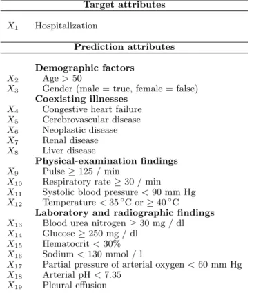
The Pneumonia PORT dataset is based on the study conducted from October 1991 to March 1994 on 2287 patients with community–acquired pneumonia from three geographical locations at five medical institu-tions. (Kapoor, 1996; Fine et al., 1997). The original PORT data were analyzed by (Fine et al., 1997), who derived a prediction rule with 30–day hospital mor-tality rate as the outcome. The authors developed a logistic regression model, which helped to identify 20 attributes that contribute the most to the mortality rate of pneumonia. To explore the anomaly detec-tion methods, we have experimented with a simpler version of the PORT dataset that records, for every patient, only the attributes identified by Fine’s study (Fine et al., 1997). The attributes are summarized in Figure 1. The output attribute corresponds to the hospitalization decision.

To study our anomaly detection methods in PORT dataset, we used 100 patient cases (out of a total of 2287 of cases). The cases picked for the study consisted of 21 cases that were found anomalous according to a

simple Na¨ıve Bayes detector (with detection threshold 0.05) that was trained on all cases in the database. The remaining 79 cases were selected randomly from the rest of the database. Each of the 100 cases was then evaluated independently by a panel of three physicians. The physicians were asked whether they agree with the hospitalization decision or not. Using panel’s answers, the admission decision was labeled as anomalous when (1) at least two physicians disagreed with the actual admission decision that was taken for a given patient case or (2) all three indicated they were unsure (gray area) about the appropriateness of the management decision. Out of 100 cases, the panel judged 23 as anomalous hospitalization decisions; 77 patient cases were labeled as not being anomalous. The assessment of 100 cases by the panel represented the correct as-sessment of unusual hospitalization decisions.

4.2. HIT dataset

Heparin–induced thrombocytopenia (HIT) (Warkentin & Greinacher, 2004) is a transient pro–thrombotic disorder induced by Heparin exposure with subsequent thrombocytopenia and associated thrombosis. HIT is a condition that is life–threatening if it is not detected and managed properly. The pres-ence of HIT is tested by a special lab assay: Heparin Platelet factor 4 antibody (HPF4).

The HIT dataset used in our experiment was built from de–identified data selected from 4273 records of post–surgical cardiac patients treated at one of the University of Pittsburgh Medical Center (UPMC) teaching hospitals. The data for the was obtained with University of Pittsburgh Institutional Review Board approval. The data collected for patients was obtained from the MARS system, which serves as an archive for much of the data collected at UPMC. The records for individual patients included discharge records, demo-graphics, all labs and tests (including standard and all special tests), two medication databases, and a finan-cial charges database. For the purpose of this exper-iment the data were preprocessed and used to build a dataset of 45767 patient state examples for which the HPF4 test–order decision (order vs. no–order) was considered and evaluated. The patient states were gen-erated automatically at discrete time points marked by the arrival of a new platelet result, a key feature used in the HIT detection. A total of 271 HPF4 or-ders were associated with these states (prior of a test order is 0.59%) Each data–point generated consisted of a total of 45 features that included recent platelets, platelet trends, platelet drops from nadir and the first platelet value, a set of similar values for hemoglobin and hemoglobin trends, whether a transfusion was

(6)

done in last 48 hourse, an indicator of the ongoing Heparin treatment and the total time on Heparin. To study the performance of our anomaly detection methods in the HIT dataset, we used 60 patient state cases (out of a total of 45767 of cases). The cases picked for the study consisted of 30 cases with the HPF4 order and 30 cases without HPF4. Each of these 60 cases was evaluated for appropriateness of HPF4 or-der by a pharmacy expert. 28 were found anomalous. 4.3. Experiments

All the experiments followed the leave–one–out scheme. That is, for each example in the dataset of patient cases (100 for PORT and 60 for HIT) evalu-ated by humans, we first learn the metric. Next, we identified the cases in E most similar to it with re-spect to that metric. The cases chosen were either the some number of closest cases (40 for PORT and 100 for HIT), or all the other cases (2286 for PORT or 45766 for HIT) in the dataset. We then learned the NB model or SVM and calculated the projection. The target example was declared anomalous if its pro-jection value fell below the detection threshold. The anomaly calls made by our algorithms were compared to the assessment of the panel and the resulting statis-tics (sensitivity, specificity) were calculated. To gain insight on the overall performance of each method we varied its detection threshold and calculated corre-sponding receiver operating characteristic (ROC). For the hospital deployment no all thresholds are accept-able. Consequently, for the evaluation we selected only that part of the ROC curve that corresponds to speci-ficity equal or greater than 95%. The 95% specispeci-ficity limit means that at most 1 in 20 normal cases analyzed may yield a false alarm.

5. Results

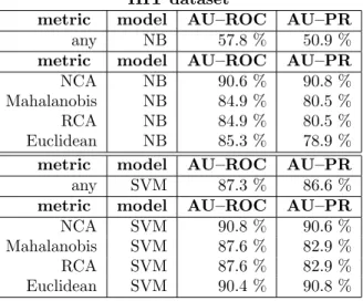
Tables 1 and 2 show the ROC statistics for the fea-sible detection range. We see that for both datasets and models, using the NCA metric and selecting the closest patients outperformed all other methods (ex-cept for NB for PORT where it ended up second best). Moreover, in most of the other cases local models (us-ing only close patients) achieved superior performance over their global counterparts. Close patients let us fit better the predictive model to the target patient, while taking all samples into the consideration biases the population. Regarding local models, performances of Na¨ıve Bayes and SVM projections are comparable. For the HIT dataset we also show traditional area under ROC for the full specificity range and PR (precision–

Target attributes

X1 Hospitalization

Prediction attributes Demographic factors

X2 Age>50

X3 Gender (male = true, female = false) Coexisting illnesses

X4 Congestive heart failure

X5 Cerebrovascular disease X6 Neoplastic disease X7 Renal disease X8 Liver disease Physical-examination findings X9 Pulse≥125 / min

X10 Respiratory rate≥30 / min

X11 Systolic blood pressure<90 mm Hg

X12 Temperature<35◦C or≥40◦C

Laboratory and radiographic findings

X13 Blood urea nitrogen≥30 mg / dl

X14 Glucose≥250 mg / dl

X15 Hematocrit<30%

X16 Sodium<130 mmol / l

X17 Partial pressure of arterial oxygen<60 mm Hg

X18 Arterial pH<7.35

X19 Pleural effusion

Figure 1.Attributes from the Pneumonia PORT dataset used in the anomaly detection study.

PORT dataset

metric model #cases area

any NB 2286 11.6 %

NCA NB 40 16.8 %

Mahalanobis NB 40 17.6 %

RCA NB 40 17.6 %

Euclidean NB 40 16.4 %

any SVM 2286 12.1 %

NCA SVM 40 19.0 %

Mahalanobis SVM 40 11.9 %

RCA SVM 40 10.4 %

Euclidean SVM 40 11.2 %

Table 1.PORT dataset: Area under the ROC curve in the feasible range of 95% – 100% specificity. Please note that the baseline value for the random choice is 2.5%, maximum is 100 %.

(7)

HIT dataset

any NB 45766 3.0 %

NCA NB 100 30.7 %

Mahalanobis NB 100 16.2 %

RCA NB 100 16.2 %

Euclidean NB 100 12.0 %

any SVM 45766 21.9 %

NCA SVM 100 30.4 %

Mahalanobis SVM 100 18.6 %

RCA SVM 100 18.6 %

Euclidean SVM 100 28.9 %

Table 2.HIT dataset: Area under the ROC curve in the feasible range of 95% – 100% specificity. Please note that the baseline value for the random choice is 2.5%, maximum is 100 %.

HIT dataset

metric model AU–ROC AU–PR

any NB 57.8 % 50.9 %

NCA NB 90.6 % 90.8 %

Mahalanobis NB 84.9 % 80.5 %

RCA NB 84.9 % 80.5 %

Euclidean NB 85.3 % 78.9 %

any SVM 87.3 % 86.6 %

NCA SVM 90.8 % 90.6 %

Mahalanobis SVM 87.6 % 82.9 %

RCA SVM 87.6 % 82.9 %

Euclidean SVM 90.4 % 90.8 %

Table 3.HIT dataset: Area under the Receiver Operating Characteristic and Precision–Recall curves.

recall) curve in table 3. The results in table 3 are qualitatively equivalent to those in table 2.

6. Conclusions

Conditional anomaly detection is a promising method-ology for detecting unusual events that may corre-spond to the medical errors or unusual outcomes. We have proposed a new anomaly detection approach that uses the discriminative projection techniques to identify anomalies. The method generalizes previ-ously proposed probabilistic anomaly detection frame-work (Hauskrecht et al., 2007). The advantage of the method is that it performs fully unsupervised and with the minimum input from the domain expert.

The new method was tested on the new Heparin in-duced thrombocytopenia dataset with over 40kpatient state entries. The experiments demonstrated that our evidence–based anomaly detection methods can detect clinically important anomalies very well, with the de-tector based on the NB or SVM projections.

Despite initial encouraging results, our current ap-proach can be further refined and extended. For exam-ple, instance–based (local) models tested in this paper always used a fixed number of 40 or 100 closest pa-tients (or more, if the distances were the same). How-ever, the patient’s neighborhood and its size depend on the patient and data available in the database. We plan to address the problem by developing methods that are able to automatically identify and select only patients that are close enough for the case in hand.

7. Acknowledgements

The research presented in this paper was funded by the grants R21–LM009102–01A1 and R01–LM06696 from the National Library of Medicine and the grant IIS–0325581 from National Science Foundation. The authors would like to thank Michael Fine who allowed us to use the PORT data.

References

Aha, D. W., Kibler, D., & Albert, M. K. (1991). Instance-based learning algorithms. Mach. Learn., 6, 37–66.

Bar-Hillel, A., Hertz, T., Shental, N., & Weinshall, D. (2005). Learning a mahalanobis metric from equiva-lence constraints. Journal of Machine Learning Re-search,6, 937–965.

(8)

machines for pattern recognition. Data Mining and Knowledge Discovery,2, 121–167.

Domingos, P., & Pazzani, M. J. (1997). On the opti-mality of the simple bayesian classifier under zero-one loss. Machine Learning,29, 103–130.

Eskin, E. (2000). Anomaly detection over noisy data using learned probability distributions. Proc. 17th International Conf. on Machine Learning(pp. 255– 262). Morgan Kaufmann, San Francisco, CA. Fine, M. J., Auble, T. E., Yealy, D. M., Hanusa, B. H.,

Weissfeld, L. A., Singer, D. E., Coley, C. M., Marrie, T. J., & Kapoor, W. N. (1997). A prediction rule to identify low-risk patients with community-acquired pneumonia.New England Journal of Medicine,336, 243–250.

Goldberger, J., Roweis, S. T., Hinton, G. E., & Salakhutdinov, R. (2004). Neighbourhood compo-nents analysis. NIPS.

Hauskrecht, M., Valko, M., Kveton, B., Visweswaram, S., & Cooper, G. (2007). Evidence-based anomaly detection. Annual American Medical Informatics Association Symposium(pp. 319–324).

Heckerman, D. (1995). A tutorial on learning with bayesian networks (Technical Report). Microsoft Research, Redmond, Washington. Revised June 96. Kapoor, W. N. (1996). Assessment of the variantion and outcomes of pneumonia: Pneumonia patient outcomes research team (PORT) final report (Tech-nical Report). Agency for Health Policy and Re-search (AHCPR).

Lauritzen, S., & Spiegelhalter, D. (1988). Local com-putations with probabilities on graphical structures and their application to expert systems. Journal of Royal Statistical Society,50, 157–224.

Mahalanobis, P. (1936). On the generalized distance in statistics. Proc. National Inst. Sci. (India) (pp. 49–55).

Pearl, J. (1988). Probabilistic reasoning in intelligent systems: networks of plausible inference. San Fran-cisco, CA, USA: Morgan Kaufmann Publishers Inc. Shental, N., Hertz, T., Weinshall, D., & Pavel, M. (2002). Adjustment learning and relevant compo-nent analysis. ECCV ’02: Proceedings of the 7th European Conference on Computer Vision-Part IV (pp. 776–792). London, UK: Springer-Verlag.

Vapnik, V. N. (1995).The nature of statistical learning theory. New York, NY, USA: Springer-Verlag New York, Inc.

Warkentin, T. E., & Greinacher, A. (2004). Heparin-induced thrombocytopenia: recognition, treatment, and prevention: the seventh accp conference on an-tithrombotic and thrombolytic therapy. Chest,126, 311S–337S.

Wong, W. K., Moore, A., Cooper, G., & Wagner, M. (2003). Bayesian network anomaly pattern detection for disease outbreaks. Proceedings of the 20th Inter-national Conference on Machine Learning (ICML-2003).