Why Don‘t We See Poverty Convergence?
Martin Ravallion1
Development Research Group, World Bank 1818 H Street NW, Washington DC, 20433, USA
Abstract: We see signs of convergence in average living standards amongst
developing countries and of greater progress against poverty in faster growing economies. Yet we do not see poverty convergence; the poorest countries are not enjoying higher rates of poverty reduction. The paper tries to explain why. Consistently with some growth theories, analysis of a new data set for 100 developing countries reveals an adverse effect on consumption growth of high initial poverty incidence at a given initial mean. Starting with a high incidence of poverty also entails a lower rate of progress against poverty at any given growth rate (and conversely poor countries tend to experience less steep increases in poverty during recessions). Thus, for many poor countries, the growth advantage of starting out with a low mean is lost due to their high poverty rates. The size of the middle class—measured by developing-country, not Western, standards— appears to be an important channel linking current poverty to subsequent growth and poverty reduction. However, high current inequality is only a handicap if it entails a high incidence of poverty relative to mean consumption.
Keywords: Poverty trap, middle class, inequality, economic growth
JEL: D31, I32, O15
1 These are the views of the author and should not be attributed to the World Bank or any affiliated
organization. Address: mravallion@worldbank.org. The author is grateful to Shaohua Chen and Prem Sangraula for help in setting up the data set used here. Helpful comments were received from Karla Hoff, Aart Kraay, Luis Servén, Dominique van de Walle, participants at presentations at the World Bank, the Courant Research Center, Göttingen, the 2009 meeting in Buenos Aires of the Network on Inequality and Poverty and the Institute of Social Sciences, Cornell University.
1.
Introduction
Two prominent stylized facts about economic development are that there is an advantage of backwardness, such that on comparing two otherwise similar countries the one with the lower initial mean income will tend to see the higher rate of growth, and that there is an advantage of growth, whereby a higher mean income tends to come with a lower incidence of absolute poverty. Past empirical support for both stylized facts has almost invariably assumed that the dynamic processes for growth and poverty reduction do not depend directly on the initial level of poverty. Under that assumption, the two stylized facts imply that we should see poverty
convergence: countries starting out with a high incidence of absolute poverty (reflecting a lower mean) should enjoy a higher subsequent growth rate and (hence) higher proportionate rate of poverty reduction. Indeed, as will be demonstrated later, the mean and the poverty rate will have the same speed of convergence in widely-used log-linear models.
That poses a puzzle. As this paper will also show, there is no sign of poverty convergence amongst developing countries, let alone a similar speed of convergence to that found for the mean. The overall incidence of poverty is falling in the developing world, but no faster (in proportionate terms) in its poorest countries.2 Clearly something is missing from the story. Intuitively, one hypothesis is that either the growth process in the mean, or the impact of growth on poverty, depends directly on the initial poverty rate, in a way that nullifies the ―advantage of backwardness.‖ Later I will point to a number of theoretical arguments as to how this can happen.
To test this hypothesis, a new data set was constructed for this paper from household surveys for almost 100 developing countries, each with two or more surveys over time. These data are used to estimate a model in which the rate of progress against poverty depends on the rate of growth in the mean and various parameters of the initial distribution—encompassing those identified in the literature—while the rate of growth depends in turn on initial distribution as well as the initial mean. The model is subjected to a number of tests, including alternative functional forms, sample selection by type of survey, and alternative measures are used for the key variables. A sub-sample with three or more surveys is also used to test robustness to
2 Note that poverty convergence is defined in proportionate rather than absolute terms, in keeping with usage
the in the growth literature. The absence of poverty convergence by this definition implies that poorer countries tend to see larger absolute reductions in their poverty rate.
different specification choices, including treating initial distribution as endogenous by treating lagged initial distribution as excludable.
The results suggest that mean-convergence is counteracted by two distinct ―poverty effects.‖ First, there is an adverse direct effect of high initial poverty on growth—working against convergence in mean incomes. Second, high initial poverty dulls the impact of growth on poverty; the poor enjoy a lower share of the gains from growth in poorer countries. On balance there is little or no systematic effect of starting out poor on the rate of poverty reduction. Other aspects of the initial distribution play no more than a secondary role. High initial inequality only matters to growth and poverty reduction in so far as it entails a high initial incidence of poverty relative to the mean. Countries starting out with a small middle class—judged by developing country rather than Western standards—face a handicap in promoting growth and poverty reduction though this too is largely accountable to differences in the incidence of poverty.
2.
Past theories and evidence
Growth theories incorporating credit-market failure suggest that high inequality reduces an economy‘s aggregate efficiency and (hence) growth rate.3
The market failure is typically attributed to information asymmetries—that lenders are poorly informed about borrowers. The key analytic feature of such models is a suitably nonlinear relationship between an individual‘s initial wealth and her future wealth (the ―recursion diagram‖). The economic rationale for a nonlinear recursion diagram is that the credit market failure leaves unexploited opportunities for investment in physical and human capital and that there are diminishing marginal products of capital. Then mean future wealth will be a quasi-concave function of the distribution of current wealth; thus higher current inequality implies lower future mean wealth at a given value of current mean wealth. Models with such features include Galor and Zeira (1993), Benabou (1996), Aghion and Bolton (1997) and Banerjee and Duflo (2003).
But is it inequality that matters, or something else, such as poverty or the size of the middle class? Inequality is obviously not the same thing as poverty; inequality can be reduced
3
There are a number of surveys including Perotti (1996), Hoff (1996), Aghion et al. (1999), Bardhan et al. (2000), Banerjee and Duflo (2003), Azariadis (2006) and World Bank (2006, Chapter 5). Borrowing constraints are not the only way that inequality can matter to growth. Another class of models is based on the idea that high inequality restricts enhancing cooperation, such that key public goods are underprovided or efficiency-enhancing policy reforms are blocked (Bardhan et al., 2000). Other models argue that high inequality leads democratic governments to implement distortionary redistributive policies, as in Alesina and Rodrik (1994).
without a lower poverty measure by redistributing income amongst the non-poor, and poverty can be reduced without lower inequality. (Similarly, efforts to help the middle-class may do little to relieve current poverty.) In fact there is another implication of credit market failures that has received very little attention. 4 The following section studies one theoretical model from the literature more closely and shows that the simple fact of a credit constraint implies that unambiguously higher current poverty incidence—defined by any poverty line up to the minimum level of initial wealth needed to not be liquidity constrained in investment—yields lower growth at a given level of mean current wealth.
This is not the only argument suggesting that poverty is a relevant parameter of the initial distribution. Lopez and Servén (2009) introduce a subsistence consumption requirement into the utility function in the model of Aghion et al. (1999) and show that higher poverty incidence (failure to meet the subsistence requirement) implies lower growth. Another example can be found in the theories that have postulated impatience for consumption (high time preference rates possibly associated with low life expectancy) and hence low savings and investment rates by the poor (see, for example, Azariadis, 2006). Here too, while the theoretical literature has focused on initial inequality, it can also be argued that a higher initial incidence of poverty means a higher proportion of impatient consumers and hence lower growth.
Yet another example is found by considering how work productivity is likely to be affected by past nutritional and health status. Only when past nutritional intakes have been high enough (above basal metabolic rate) will it be possible to do any work, but diminishing returns to work will set in later; see the model in Dasgupta and Ray (1986). Following Cunha and
Heckman (2007), this type of argument can be broadened to include other aspects of child development that have lasting impacts on learning ability and earnings as an adult. By
implication, having a larger share of the population who grew up in poverty will have a lasting negative impact on an economy‘s aggregate output.
There are also theoretical arguments involving market and institutional development, though this is not a topic that has so far received as much attention in this literature. While past theories have often taken credit-market failures to be exogenous, poverty may well be a deeper causative factor in financial development (as well as an outcome of the lack of financial
development). For example, given fixed cost of lending (both for each loan and for setting up the lending institution), liquidity constraints can readily emerge as the norm in very poor societies.
A strand of the theoretical literature has also pointed to the possibilities for multiple equilibria in nonlinear dynamic models, whereby the lowest equilibrium is a poverty trap (―low-level attractor‖). Essentially, the recursion diagram now has a low-(―low-level non-convexity, whereby a minimum level of current wealth is essential before any positive level of future wealth can be reached. In poor countries, the nutritional requirements for work can readily generate such dynamics, as illustrated by the model of Dasgupta and Ray (1986). Such a model predicts that a large exogenous income gain may be needed to attain a permanently higher income and that seemingly similar aggregate shocks can have dissimilar outcomes; growth models with such features are also discussed in Day (1992) and Azariades (1996, 2006) amongst others. Sachs (2005) has invoked such models to argue that a large expansion of development aid would be needed to assure a permanently higher average income in currently poor countries.
2.1
A model of aggregate growth with micro borrowing constraints
I now explore one of these models more fully. Banerjee and Duflo (2003) provide a simple but insightful growth model with borrowing constraints. Someone who starts her productive life with sufficient wealth is able to invest her unconstrained optimal amount, equating the (declining) marginal product of her capital with the interest rate. But the ―wealth poor,‖ for whom the borrowing constraint is binding, are unable to do so. Banerjee and Duflo show that higher inequality in such an economy implies lower growth. However, they do not observe that their model also implies that higher current wealth poverty for a given mean wealth also implies lower growth. The following discussion uses the Banerjee-Duflo model to illustrate this hypothesis, which will be tested later in the paper.
The basic set up of the Banerjee-Duflo model is as follows. Current wealth, wt, is
distributed across individuals according to the cumulative distribution function, p Ft(w), giving the population proportion p with wealth lower than w at date t. It will be analytically easier to work with the quantile function, wt(p) (the inverse of Ft(w)). The credit market is imperfect, such that individuals can only borrow up to times their wealth. Each person has a strictly concave production function yielding output h(k) from a capital stock k. Given the rate
of interest r (taken to be fixed) the desired capital stock is k*, such that h(k*)r. Those with initial wealth less than k*/(1) are credit constrained in that, after investing all they can, they still find that h(kt)r, while the rest are free to implement k*. A share 1(0,1)of current wealth is consumed, leaving for the next period.
Under these assumptions, the recursion diagram takes the form:
] ) ) 1 (( [ ) ( 1 t t t t w h w rw w for wt k*/(1) (1.1) ] ) ( ) ( [h k* wt k* r for wt k*/(1) (1.2)
Plainly, (wt) is strictly concave up to k*/(1) and linear above that. Mean future wealth is:
0 1 [wt(p)]dp t (2)By standard properties of concave functions, we have:
Proposition 1: (Banerjee and Duflo, 2003, p.277): “An exogenous mean-preserving
spread in the wealth distribution in this economy will reduce future wealth and by implication the growth rate.”
However, the Banerjee-Duflo model has a further implication concerning poverty, as
another aspect of the initial distribution. Let Ht Ft(z) denote the headcount index of poverty (―poverty rate‖) in this economy when the poverty line is z. I assume that zk*/(1) and let
)] 1 /( [ * * k F
Ht t . Using (1.1) and (1.2) we can re-write (2) as:
1 * * 0 1 * * ] ) ) ( ( ) ( [ )] ( )) ( ) 1 (( [ t t H t H t t t h w p rw p dp h k w p k r dp (3)Now consider the growth effect of a mean-preserving increase in the poverty rate. I assume that
*
t
H increases and that no individual with wealth less than k*/(1)becomes better off, implying that wt(p)/Ht*0 for all
*
t H
p . If this holds then I will say that poverty is unambiguously higher. It is readily verified that:5
* * 0 * 0 * * 1 [ (( 1) ( ))( 1) ] ( ) ( ) t t H t t H t t t t t dp H p w r dp H p w r p w h H (4)5 Note that the function defined by equations (1.1) and (1.2) is continuous at
) 1 /(
*
The sign of (4) cannot be determined under the assumptions so far.6 However, on imposing a constant initial mean t , equation (4) simplifies to:
[ (( 1) ( )) ]( 1) ( ) 0 * 0 * * 1
t t H t t t t t dp H p w r p w h H (5)Thus we also have:
Proposition 2: In the Banerjee-Duflo model an unambiguously higher initial headcount index of poverty holding the initial mean constant implies a lower growth rate.
This model implies an aggregate efficiency cost of a high incidence of poverty. But a number of points should be noted. An inequality effect is still present—separately to the poverty effect. And the less poverty there is, the less important overall inequality is to subsequent growth prospects. Also note that the theoretical prediction concerns the level of poverty at a given initial value of mean wealth. Without controlling for the initial mean, the sign of the effect of higher poverty on growth is ambiguous. Two opposing effects can be identified. The first is the usual conditional convergence property, whereby countries with a lower initial mean (and hence higher initial poverty) tend to have higher subsequent growth. Against this, there is an adverse
distributional effect of higher poverty (Proposition 2). Which effect dominates is an empirical question.
2.2
Past evidence on growth and the initial distribution
Following Barro and Sala-i-Martin (1992), cross-country regressions for GDP growth rates have found a significant negative coefficient on initial GDP once one controls for initial conditions. A subset of the literature has used inequality as one such initial condition. Support for the view that higher initial inequality impedes growth has been reported by Alesina and Rodrik (1994), Persson and Tabellini (1994), Birdsall et al., (1995), Clarke (1995), Perotti (1996), Deininger and Squire (1998), Knowles (2005) and Voitchovsky (2005). Not all the evidence has been supportive; also see Li and Zou (1999), Barro (2000) and Forbes (2000). The main reason why the latter studies have been less supportive appears to be that they have allowed for additive country-level fixed effects in growth rates; I will return to this point.
6 If there is (unrestricted) first-order dominance, whereby ( )/ *0 t t p H
w for allp[0,1], then 0
/ *
1
t Ht . However, first-order dominance is ruled out by the fact that the mean is held constant in this
There are a number of unresolved specification issues in this literature. The aspect of initial distribution that has received almost all the attention in the empirical literature is
inequality, as typically measured by the Gini index. Wealth inequality is arguably more relevant though this has rarely been used due to data limitations.7
The popularity of the Gini index appears to owe more to its availability in secondary data compilations than any intrinsic relevance to the economic arguments.8 In the only paper I know of in which a poverty measure was used as a regressor for aggregate growth across countries, Lopez and Servén (2009) find evidence that a higher initial poverty rate retards growth. As Lopez and Servén observe, the significance of the Gini index in past studies may reflect an omitted variable bias, given that one expects (and I will later verify empirically) that inequality will be highly correlated with poverty at a given mean.
There are also issues about the relevant control variables when studying the effect of initial distribution on growth. The specification choices in past work testing for effects of initial distribution have lacked clear justification in terms of the theories predicting such effects. Consider three popular predictors of growth, namely human development, the investment share, and financial development. On the first, basic schooling and health attainments (often significant in growth regressions) are arguably one of the channels linking initial distribution to growth. Indeed, that is the link in the original Galor and Zeria (1993) model.9 Turning to the second, one of the most robust predictors of growth rates is the share of investment in GDP (Levine and Renelt, 1992); yet arguably one of the main channels through which distribution affects growth is via aggregate investment and this is one of the channels identified in the theoretical literature. Finally, consider private credit (as a share of GDP), which has been used as a measure of ―financial sector development‖ in explaining growth and poverty reduction (Beck et al., 2000, 2007). The theories discussed above based on borrowing constraints suggest that the aggregate flow of credit in the economy depends on the initial distribution.
Another set of specification issues concerns interaction effects. As Banerjee and Duflo (2003) point out, while liquidity constraints stemming from credit-market failures imply that the
7
An exception is Ravallion (1998), who studies the effect of geographic differences in the distribution of wealth on growth in China.
8 The compilation of Gini indices from secondary sources (and not using consistent assumptions) in
Deininger and Squire (1996) led to almost all the tests in the literature since that paper was published.
9 More recently, Gutiérrez and Tanaka (2009) show how high initial inequality in a developing country can
yield a political-economy equilibrium in which there is little or no public investment in basic schooling; the poorest families send their kids to work, and the richest turn to private schooling.
growth rate depends on the extent of inequality in the initial distribution, they also suggest that there will be an interaction effect between the initial mean and inequality. However, as the further analysis of the Banerjee-Duflo model in the last section suggests, the more relevant interaction effect may well be that between poverty and inequality.
Some of the literature has focused instead on testing the assumptions of these theories. The empirical evidence on poverty traps is mixed. At least some of the theoretical models of poverty traps appear to be hard to reconcile with the aggregate data; see, in particular, the discussion in Kraay and Raddatz (2007) of poverty traps that might arise from low savings (high time preference rates) in poor countries. There are also testable implications for micro data. An implication of a number of the models based on credit-market failures is that individual income or wealth at one date should be an increasing concave function of its own past value. This can be tested on micro panel data. Lokshin and Ravallion (2004) provide supportive evidence in panel data for Hungary and Russia while Jalan and Ravallion (2004) do so using panel data for China. These micro studies suggest seemingly sizeable efficiency costs of inequality. The same studies do not, however, find the properties in the empirical income dynamics that would be needed for a poverty trap. There is also evidence of nonlinear wealth effects on new business start ups in developing countries, though with little sign of a non-convexity at low levels due to lumpiness in capital requirements (Mesnard and Ravallion, 2006). Similarly, McKenzie and Woodruff (2006) find no sign of non-convexities in production at low levels amongst Mexican microenterprises. However, Hoddinott (2006) and Barrett et al (2006) find evidence of wealth-differentiated behaviors in addressing risk in rural Zimbabwe and Kenya (respectively) that are consistent with the idea of poverty traps.
Micro-empirical support for the claim that there are efficiency costs of poor nutrition and health care for children in poor families has come from a number of studies. In a recent example, an impact evaluation by Macours et al. (2008) of a conditional cash transfer scheme in Nicaragua found that randomly assigned cash transfers to poor families improved the cognitive outcomes of children through higher intakes of nutrition-rich foods and better health care. This echoes a number of findings on the benefits to disadvantaged children of efforts to compensate for family poverty; for a review see Currie (2001).
While the theories and evidence reviewed above point to inequality and/or poverty as the relevant parameters of the initial distribution, yet another strand of the literature has pointed to
various reasons why the size of a country‘s middle class can matter to the fortunes of those not (yet) so lucky to be middle class. It has been argued that a larger middle class promotes
economic growth, such as by fostering entrepreneurship, shifting the composition of consumer demand, and making it more politically feasible to attain policy reforms and institutional changes conducing to growth. Analyses of the role of the middle class in promoting entrepreneurship and growth include Acemoglu and Zilibotti (1997) and Doepke and Zilibotti (2005). Middle-class demand for higher quality goods plays a role in the model of Murphy et al. (1989). Birdsall et al. (2000) conjecture that support from the middle class is crucial to reform. Sridharan (2004) describes the role of the Indian middle class in promoting reform. Easterly (2001) finds evidence that a larger income share controlled by the middle three quintiles promotes economic growth.
So we have three contenders for the distributional parameter most relevant to growth: inequality, poverty and the size of the middle class. The fact that very few encompassing tests are found in the literature, and that these different measures of distribution are not independent, leaves one in doubt about what aspect of distribution really matters. As already noted, when the initial value of mean income is included in a growth regression alongside initial inequality, but initial poverty is an excluded but relevant variable, the inequality measure may pick up the effect of poverty rather than inequality per se. Similarly, the main way the middle class expands in a developing country is probably through poverty reduction, so it is unclear whether it is a high incidence of poverty or a small middle class that impedes growth. Similarly, a relative concept of the ―middle class,‖ such as the income share of middle quintiles, will probably be highly
correlated with a relative inequality measure, clouding the interpretation.
2.3
Growth and poverty reduction
The consensus in the literature is that higher growth rates tend to yield more rapid rates of absolute poverty reduction; see World Bank (1990, 2000), Ravallion (1995, 2001, 2007), Fields (2001) and Kraay (2006).10 This is implied by another common finding in the literature, namely that growth in developing countries tends to be distribution-neutral on average, meaning that changes in inequality are roughly orthogonal to growth rates in the mean (Ravallion, 1995, 2001; Ferreira and Ravallion, 2009). Distribution-neutrality in the growth process implies that the
changes in any standard measure of absolute poverty (meaning that the poverty line is fixed in real terms) will be negatively correlated with growth rates in the mean.
There is also evidence that inequality matters to how much a given growth rate reduces poverty (Ravallion, 1997, 2007; World Bank, 2000, 2006; Bourguignon, 2003; Lopez and
Servén, 2006). Intuitively, in high inequality countries the poor will tend to have a lower share of the gains from growth. Ravallion (1997, 2007) examined this issue empirically using household survey data over time (earlier versions of the data set used here). Ravallion (1997) found that the following parsimonious specification fits the data for developing countries well:
lnHit (1Git1)lnitit (6)
where Hit, Git and it are the headcount index, the Gini index and the mean respectively for country i at date t, 0 is the elasticity of poverty reduction to the ―distribution-corrected‖ growth rate (1Git1)lnit and it is a zero mean error term (uncorrelated with the growth rates). At minimum inequality (Git10) growth has its maximum effect on poverty (in expectation) while the elasticity reaches zero at maximum inequality (Git11). Ravallion (1997) did not find that the elasticity varied systematically with the mean, although Lopez and Servén (2006) showed that if incomes are log-normally distributed then such a variation is implied theoretically. Easterly (2009) conjectured that the initial poverty rate is likely to be the better predictor of the elasticity than initial inequality, though no evidence was provided.
3.
Data and descriptive statistics
In keeping with the bulk of the literature, the country is the unit of observation.11
However, unlike past data sets in the literature on growth empirics, this one is firmly anchored to the household surveys, in keeping with the focus on the role played by the initial distribution, which is measured from surveys. By calculating the distributional statistics directly from the primary data, some of the inconsistencies and comparability problems found in existing data compilations from secondary sources can be eliminated. However, there is no choice but to use household consumption or income, rather than the theoretically preferable concept of wealth.
11 It is known that aggregation can hide the true relationships between the initial distribution and growth,
given the nonlinearities involved at the micro level (Ravallion, 1998); identifying the deeper structural relationships would require micro data, and even then the identification problems can be formidable.
I found 99 developing and transition countries with at least two suitable household surveys since about 1980. (For about 70 of these countries there are three or more surveys.) For the bulk of the analysis I restrict the sample to the 92 countries in which the earliest available survey finds that at least some households lived below the average poverty line for developing countries (described below).12 This happens mechanically given that log transformations are used. However, it also has the defensible effect of dropping a number of the countries of Eastern Europe and Central Asia (EECA) (including the former Soviet Union); indeed, all of the
countries with an initial poverty rate (by developing country standards) of zero are in EECA. As is well known, these countries started their transitions from socialist command economies to market economies with very low poverty rates, but poverty measures then rose sharply.13 The earliest available surveys pick up these low poverty rates, with a number of countries having no sampled household living below the poverty lines typical of developing countries. With the subsequent rise in poverty incidence, this looks like ―convergence,‖ but it has little or nothing to do with neoclassical growth processes—rather it is a ―policy convergence‖ effect associated with the transition. The experience of these countries is clearly not typical of the developing world.
The longest spell between two surveys is used for each country. Both surveys use the same welfare indicator, either consumption or income per person, following standard
measurement practices. When both are available, consumption is preferred, in the expectation that it is both a better measure of current economic welfare and that it is likely to be measured with less error than incomes;14three-quarters of the spells use consumption.
Naturally the time periods between surveys are not uniform across countries. The median year of the first survey is 1991 while the median for the second is 2004. The median interval between surveys is 13 years and it varies from three to 27 years. All changes between the surveys
are annualized. Given the most recent household survey for date ti in country i and the earliest
available survey for date ti i, the proportionate annualized difference (―growth rate‖) for the variable x is denoted gi(xit)ln(xit/xit)/ (dropping the i subscript on t and for brevity). National accounts (NAS) data and social indicators are also used, matched as closely as possible
12 The data set was constructed from PovcalNet in December 2008. Seven countries were dropped because
the poverty rate was zero in the earliest surveys.
13 Prior to the global financial crisis there were signs that poverty measures were finally falling in the region,
since the later 1990s; see Chen and Ravallion (2008).
to survey dates. All monetary measures are in constant 2005 prices (using country-specific Consumer Price Indices) and are at Purchasing Power Parity (PPP) using the individual consumption PPPs from the 2005 International Comparison Program (World Bank, 2008).
Poverty is mainly measured by the headcount index (Hit), given by the proportion of the population living in households with consumption per capita (or income when consumption is not available) below $2.00 per day at 2005 PPP, which is the median poverty line amongst
developing countries.15 Let Fit(z) denote the distribution function for country i at date t; then )
2 (
it it F
H . In 2005, $2 a day was also very close to the median consumption per person in the developing world. This line is clearly somewhat arbitrary; for example, there is no good reason to suppose that $2 a day corresponds to the point where credit constraints cease to bite, but nor is there any obviously better basis for setting a threshold. I will also consider a lower line of $1.25 a day and a much higher line of $13 a day in 2005, corresponding to the US poverty line.16
Inequality is measured by the usual Gini index (Git)—half the mean absolute difference between all pairs of incomes normalized by the overall mean.
The size of the middle class (MCit) is measured by the proportion of the population
living between $2 and $13 a day (following Ravallion, 2009); so MCit Fit(13)Fit(2).17 These bounds are also somewhat arbitrary, although this definition appears to accord roughly with the idea of what it means to be ―middle class‖ in China and India (Ravallion, 2009). By contrast, those living above $13 a day can be thought of as the ―middle class‖ by Western standards; the share of the ―Western middle class‖ is 1Fit(13). These are interpretable as absolute measures of the middle class. I also calculated a relative definition of the middle class,
namely the consumption or income share controlled by the middle three quintiles (MQit), as used by Easterly (2001).
Table 1 provides summary statistics for both the earliest and latest survey rounds. The mean Gini index stayed roughly unchanged at about 42%. The initial index ranged from 19.4%
15 This is based on the compilation of national poverty lines presented in Ravallion et al. (2009). The methods
used in measuring poverty and inequality using these data are described in Chen and Ravallion (2008).
16
The $1.25 line is the mean of the poorest 15 countries in terma of consumption per person. $13 per person per day corresponds to the official poverty line in the US for a family of four; see Department of Health and Human Services.
(Czech Republic) to 62.9% (Sierra Leone), both around 1990. In the earliest surveys, about one quarter of the sample had a Gini index below 30% while one quarter had an index above 50%.
The average size of the middle class increased, from a mean MCit of 48% to a mean
it
MC of 53%. The middle-class expanded in 64 countries and contracted in 35. There is also a marked bimodality in the distribution of countries by the size of their middle class, as is evident
in Figure 1, which plots the kernel densities of MCit and MCit. Taking 40% as the cut-off point, 30 countries are in the lower mode and 69 are in the upper one for the most recent survey; the corresponding counts for the earliest surveys are 42 and 57.18 The relative measure of the size of the middle class behaved differently; there was little change in the mean MQ over time (Table 1) and the density function was unimodal in both the earliest and latest surveys.
Table 2 gives the correlation coefficients, focusing on the main regressors used later. The correlations point to a number of potential concerns about the inferences drawn from past
research. The Gini index is highly (negatively) correlated with the income share of the middle three quintiles (r=-0.971 for the earliest surveys and -0.968 for the latest). The poverty measures
are also strongly correlated with the survey means; lnHitand lnit have a correlation of -0.851 (while it is -0.836 for lnFit(1.25) and lnit). The least-squares elasticity of lnHit
with respect to the initial survey mean (i.e., the regression coefficient of lnHitonlnit) is -1.305 (t=13.340). (All t-ratios in this paper are based on White standard errors.) There is a very high correlation between the poverty measures using $1.25 a day and $2.00 a day (r=0.974). There are weaker correlations between the two poverty measures and the initial Gini index (r= 0.241 and 0.099 for z=1.25 and z=2.00). However, there is also a strong multiple correlation between the poverty measures (on the one hand) and the log mean and log inequality (on the
other); for example, regressing lnHiton lnit and lnGit one obtains R2=0.802. The log Gini index also has a strong partial correlation with the log of the poverty rates holding the log
mean constant (t=4.329 for lnHit).
The size of the middle class is also highly correlated with the poverty rate; the correlation
coefficient between MCit and Hitis -0.975; 95% of the variance in the initial size of the
18 For further discussion of the developing world‘s rapidly expanding middle class, and the countries left
middle class is accountable to differences in the initial poverty rate. (The bimodality in terms of the size of the middle class in Figure 1 reflects a similar bimodality in terms of the $2 a day
poverty rate.) Across countries, 80% of the variance in the changes over time in MCitcan also be
attributed to the changes inHit.19 The absolute and relative measures of the size of the middle class are positively correlated but not strongly so.
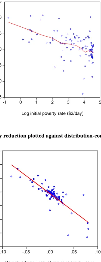
There is a strong correlation between the rate of poverty reduction and the ordinary growth rate in the survey mean (confirming the studies reviewed in section 2). Figure 2 plots the
rate of poverty reduction (gi(Hit)) against gi(it). The regression line in Figure 2 has a slope of -1.372 (t=-5.948) with R2=0.363.
Since the time period between surveys ( ) figures in the calculation of the growth rates it might be conjectured that poorer countries have longer periods between surveys, biasing the later results. Table 2 also gives the correlation coefficients between and the various measures of initial distribution. The correlations are all small.
While this paper focuses mainly on the developing world as a whole, one region stands
out: Sub-Saharan Africa (SSA). By the $2.00 a day line, the mean of Hit for SSA is 76.04% as compared to 29.51% for non-SSA countries; the difference is significant (t=8.84). Similarly, in terms of the size of its middle class, SSA is more concentrated in the lower mode in Figure 1. Two-thirds (20 out of 29) of SSA countries are in the lower mode for the earlier survey round;
the corresponding means of MCitwere 22.89% (s.e.=3.62%) and 59.07% (3.01%) for SSA and non-SSA countries respectively and the difference is statistically significant at the 1% level. Inequality too is higher in SSA; the mean Gini index in the earliest surveys is 0.474 (0.018) for SSA versus 0.390 (0.017) in non-SSA countries, and the difference is significant (t=7.68). There is clearly a ―SSA effect‖ in both growth and poverty reduction, though we will see that this is accountable to the other variables in the estimated models.
4.
Convergence?
Virtually all of the papers in the empirical literature reviewed in section 2 have assumed that the parameters of the dynamic processes for growth and poverty reduction are independent
19 R2 =0.826 for the regression of
it it MC
MC on Fit(2)Fit(2); the regression coefficient is -0.896
of the initial level of poverty. The easiest way to see that this assumption cannot be right is to show that the standard models imply something that is not supported by the data.
Consider the most common empirical specification for the growth process in the mean:
it it i i it ln ln 1 (7)
whereiis a country-specific effect, iis a country-specific convergence parameter and it is a zero-mean error term. (To simplify notation I assume evenly spaced data for now.) Next let the headcount index of poverty be a log-linear function of the mean:
it it i i it H ln ln (8)
where i 0 and itis a zero-mean error term. This assumes that relative distribution fluctuates around a stationary mean, with changes in distribution orthogonal to growth rates in the mean. The implied growth model for poverty is then:
* 1 * ln lnHit i i Hit it (9)
for which it is readily verified that i* ii ii and it* iti it (1i)it1. The parameters of (7) and (8) (i,i,i,i) can vary across counties but (for the sake of this argument) suppose they do so independently ofHit. Then the ―speed of convergence‖ for the
mean, lnit/lnit1 i, is the same as that for poverty: lnHit /lnHit1i. Thus we have:
Proposition 3: In standard log-linear models for growth and poverty reduction, with parameters independent of the initial level of poverty, the speed of convergence will be the same for the mean as the poverty measure.
However, this is not borne out by the data. Table 3 gives convergence tests for both the mean and the poverty measures, with and without controls.20 The controls included initial consumption per capita from the NAS, primary school enrollment rate, life expectancy at birth, and the price index of investment goods from Penn World Tables (6.2), which is a widely-used measure of market distortions; all three variables are matched as closely as possible to the date of the earliest survey. The survey means exhibit convergence with a coefficient of -0.013
20
The test is the regression coefficient of gi(it) on lnit. Alternatively one can estimate the nonlinear
regression g()[(1e)/]ln . This gave a very similar result to (1) in Table 4, namely ˆ 0.012. (t=-2.865). Clearly, the approximation that e 1 works well.
3.412) without the controls and -0.042 (t=-7.435) with them. But this not true of the poverty measures. Indeed the proportionate rates of poverty reduction are orthogonal to initial levels.21 Figure 3 plots the data, and gives a non-parametric regression line.
Clearly these results do not support the idea that the mean and the poverty measure have the same speed of convergence; indeed, there is no convincing sign of poverty convergence. The rest of this paper will try to explain why. In terms of the model above, it will be shown that the
parameteriis a decreasing function of the initial poverty rate while the elasticity of poverty to the mean,i, is a decreasing function of the initial level of poverty.
5.
The relevance of initial poverty to growth in the mean
As discussed in section 2, initial distribution can matter to the rate of poverty reduction through two distinct channels, namely the growth rate and the elasticity of poverty to the mean. I postulate a simple triangular model in which rate of growth depends in turn on initial distribution while the rate of progress against poverty depends on the interaction between the growth rate and the initial distribution. This section focuses on the first relationship; section 6 turns to the second.
The section begins with benchmark regressions of growth on the initial mean and initial poverty rate. A causal interpretation of these regressions requires that the initial distribution (in the earliest survey used to construct each spell) is exogenous to the subsequent pace of growth. This can be questioned. I shall test encompassing models with controls for other factors. I also provide results for an instrumental variables estimator under widely-used (though still
questionable) exclusion restrictions.
5.1
Benchmark regression for growth
Table 4 gives estimates of the following regression:22
it it it it i H g ( )ln ln (10) 21
For the $1.25 line the corresponding regression coefficient was -0.005 with t=-0.393; at the other extreme, for the $13 line it was -0.009 (t=-0.480). Again, the nonlinear specification gave a very similar result.
22
The regressions are consistent with a derivative of lnit with respect to lnit that is less than unity, but
fades toward zero at sufficiently long gaps between survey rounds; for example, column (1) in Table 4 implies a derivative that is less than unity for 29 years; the largest value of in the data is 27 years.
The estimates in column (1) suggest that differences in the initial poverty rate have sizeable negative impacts on the growth rate at a given initial mean. A one standard deviation increase in
it H
ln would come with 0.021 (2% points) decline in the growth rate for the survey mean.
The fact that a significant (partial) correlation with the initial poverty rate only emerges when one controls for the initial mean is suggestive of an adverse distributional effect of high poverty. However, it is not simply a ―relative poverty‖ effect, stemming from the variance in absolute poverty attributable to differences in relative distribution. This is evident in the fact that the convergence parameter increases considerably when one adds the initial poverty measure as a
regressor. Dropping lnHitfrom (10) the coefficient on lnit falls to -0.013 (t=-3.413). The presence of the poverty rate as a regressor magnifies the convergence parameter, suggesting that the fact that the absolute poverty rate depends on the mean is also playing a crucial role in determining its significance in these regressions—working against the convergence effect.
It might be conjectured that the effect of lnHitin (10) reflects a misspecification of the functional form for the convergence effect, noting that the poverty measure is a nonlinear
function of mean income. To test for this, I re-estimated (10) using cubic functions of lnit to control for the initial mean. While I found some sign of higher-order effects of lnit, these made very little difference to the regression coefficient on the poverty rate in the augmented
regression; the coefficient on lnHitin column (1) in Table 4 became -0.018 (t=-3.547). There is, however, a marked nonlinearity in the relationship, which is being captured by
the log transformation of Hitin (10). If one usesHitrather than lnHiton the same sample, the negative effects are still evident but they are much less precisely estimated, with substantially
lower t-ratios—a t-ratio of -1.292 for the coefficient onHit—though in both cases the effects
come out somewhat more strongly if one adds a squared term in Hitto pick up the nonlinearity, with both the linear and squared terms significant at the 10% level or better.
A simple graphical test for misspecification of the functional form in (10) is to plot
it it
i
along with a locally-smoothed (non-parametric) regression line. The relationship is close to linear in the log poverty rate.23 The log transformation appears to be the right functional form.
The more relevant poverty line is that using the $2.00 a day line. On replacing lnHitby
) 25 . 1 (
lnFit in (10) the poverty rate still had a negative coefficient but it was not significant at the 5% level. I also estimated the following specification:
it it it it it it i H F F g( )ln 1[ln ln (1.25)]2ln (1.25)) (11) The estimate of 12 was -0.010, but was not significantly different from zero (t=-0.801), suggesting that (10) is the correct specification.
The results were also robust to using the poverty gap index instead of the headcount index; the corresponding version of (10) was similar, with a coefficient on the log of the poverty gap index of -0.011, with t-ratio of -2.338. However, the fit is better using the headcount index.
Recall that the sample in estimating (10) used both consumption and income surveys, and that the latter may have more measurement error. Estimating the regression solely on
consumption surveys strengthened the result; analogously to (10) one obtains column (2) of Table 4. The conditional convergence effect is even stronger, as is the poverty effect.
The results are robust to using NAS consumption growth instead (Table 4). The notable
differences are that the convergence parameter in (10) is lower, ˆ0.02 (column 3, Table 4) and that the headcount index based on the $1.25 line is a slightly stronger predictor of the NAS consumption growth. (The results using NAS consumption growth were less sensitive to the choice of poverty line between $2.00 and $1.25 a day.)
Another way to use NAS consumption is as a control for other initial conditions influencing the long-run value of the survey mean. Augmenting (10) with this extra control variable gives, for the full sample:
gi(it) 0.181 0.050lnit 0.011lnHit 0.022lnCit ˆit ) 682 . 3 ( ) 382 . 2 ( ) 817 . 6 ( ) 942 . 3 ( R2=0.288; n=87 (12)
And for the sample of consumption surveys:
gi(it) 0.232 0.061lnit 0.017lnHit 0.025lnCit ˆit ) 346 . 3 ( ) 624 . 3 ( ) 507 . 6 ( ) 868 . 4 ( R 2 =0.317; n=66 (13)
The results are consistent with the expectation that lnCit is picking up long-run differences. The poverty effect remains evident, though with a lower coefficient.
23 In both cases I have scaled the vertical axis to accord with the sample mean growth rate by using the
5.2
Further tests on the subsample with three surveys
One can form a subsample of about 70 countries with at least three household surveys. When there were more than three surveys I picked the one closest to the midpoint of the interval between the latest survey and the earliest.
There are at least four ways one can exploit the extra round of surveys. The first is to test for convergence more robustly to measurement errors.24 One way of doing this is to calculate the trend over the three surveys and test if this is correlated with the starting value. I estimated the trend for each country by regressing the logs of the three (date-specific) means for that country on time and similarly for the headcount indices. Convergence in the mean was still evident; the regression coefficient of the estimated trend on the log mean from the earliest survey was -0.009 (t=-2.052), which is significant at the 4% level. And again there was no significant correlation between these trends in poverty reduction and the initial poverty measures; the regression coefficient of the estimated trend on the log headcount index from the earliest survey was 0.007 (t=0.805). Another method is to form means from the first two surveys and look at their
relationship with the changes observed between the last survey and the middle one. Define the
mean from the first two surveys asMi(xit2)(xit2 xit12)/2 while the growth rate is
2 / ) / ln( ) ( 2 it it it i x x x
g . Using this method, unconditional mean convergence was no longer
evident (though conditional convergence was still found) but there was an indication of poverty
divergence; regressing gi(Hit) (the proportionate change in the poverty measure between the
middle and final rounds) on ( )
2
it i H
M ; the coefficient was 0.029, which is significant at the 6%
level (t=1.901). There is still some contamination due to measurement error in these tests. Yet
another method is to regress gi(xit) on the measure from the earliest survey (
2 1
lnit ); the
result was similar, namely little sign of (unconditional) mean convergence but mild divergence for poverty (a coefficient of 0.027 with t=1.819).
24 As is well known, measurement errors can create spurious signs of convergence; if the initial mean is over-
(under-) estimated then the subsequent growth rate will be lower (higher).clearly stems in part at least from this problem. It is notable that thecoefficient drops using only the consumption surveys (Table 4) or NAS
consumption. However, significant conditional convergence in the means (including those only from consumption surveys) and NAS consumption is still evident (Table 4).
Secondly, the subsample can be used to form inter-temporal averages, to reduce the attenuation biases in the benchmark regression due to measurement error; equation (10) can be re-estimated in the form:
it it i it i it i M M H g( )ln ( )ln ( ) 2 2 (14)
Column (4) of Table 4 gives the results. The regression coefficients are larger (in absolute value), consistent with the presence of attenuation bias in the earlier regressions. The standard errors also fall noticeably. This strengthens the earlier results based on equation (10).
The third way of using the extra survey rounds is as a source of instrumental variables (IVs). Growth rates between the middle and last survey rounds were regressed on the mean and distributional variables for the middle round but treating the latter as endogenous and retaining
the data for the earliest survey round as a source of IVs. Letting i now denote the length of spell
i (=1,2), the model becomes:
it it it it i H g 2 2 ln ln ) ( (15)
The instrumental variables were
2 1 lnit , 2 1 lnCit , 2 1 lnGit , ln ( ) 2 1 z Fit (z=1.25, 2.00)
and 1. The first-stage regressions for lnit2 and lnHit2 had R
2
=0.884 (F=61.06) and
R2=0.796 (F=31.30) respectively. The Generalized Methods of Moments (GMM) estimates of (15) are found in Table 4, Column (5). (I also give the corresponding result using NAS
consumption in column (6).) We see that the finding that a higher initial poverty rate implies a lower subsequent growth rate (at given initial mean) is robust to allowing for the possible endogeneity of the initial mean and initial poverty rate, subject to the usual assumption that the above instrumental variables are excludable from the main regression. Analogously to equation
(12.1), on adding
2
lnCit to specification (5) in Table 4, and treated it as exogenous, one obtains
(using the same set of instruments):
it it it it it i H C g ( ) 0.235 0.066ln 0.022ln 0.035ln ˆ ) 481 . 4 ( ) 954 . 3 ( ) 407 . 4 ( ) 731 . 3 ( (16) Dropping 2
lnCit from the set of IVs gives instead:
it it it it it i H C g ( ) 0.144 0.041ln 0.016ln 0.025ln ˆ ) 288 . 3 ( ) 634 . 2 ( ) 206 . 2 ( ) 815 . 1 ( (17)
Finally, one can use the subsample is to estimate a specification with country-fixed effects, which sweep up any confounding latent heterogeneity in growth rates at country level.
The main results were not robust to this change. Regressing the change in annualized growth rates ( ( ) ( ) 2 it i it i g
g ) on ln(it2/it12) and ln(Hit2 /Hit12), the coefficient on the
former remained significant but the poverty rate ceased to be so.
However, it is hard to take fixed-effects growth regressions seriously with these data. While this specification addresses the problem of time-invariant latent heterogeneity it is
unlikely to have much power for detecting the true relationships given that the changes over time in growth rates will almost certainly have a low signal-to-noise ratio. Simulation studies have found that the coefficients on growth determinants are heavily biased toward zero in fixed-effects growth regressions (Hauk and Wacziarg, 2009).25 I suspect that the problem of time-varying measurement errors in both growth rates and initial distribution is even greater in the present data set, possibly reflecting survey comparability problems over time.
The problem of a low signal-to-noise ratio in the changes in growth rates can be illustrated if we consider the relationship between the two measures of the mean used in this
study, namely that from the surveys (it) and that from the private consumption component of domestic absorption in the national accounts (Cit). Table 5 gives the levels regression in logs,
which implies an elasticity of ittoCit of 0.75 (R2=0.82) for the latest survey rounds.26 Using a country-fixed effects specification in the levels, the elasticity drops to 0.46 while with fixed-effects in the growth rates (using the subsample with at least three surveys) it drops to 0.09 (R2=0.07), which must be considered an implausibly low figure, undoubtedly reflecting substantial attenuation bias due to measurement error in the changes in growth rates.
5.3
Encompassing regressions
It might be conjectured that the poverty measures (at given initial means) are picking up other aspects of the initial distribution, such as inequality (the variable identified in almost all the empirical literature, as discussed in section 2). Simply adding the log of the initial Gini index to equation (10) does not change the result; the coefficient on the Gini index is not significantly
different from zero; the coefficient on lnHitremains (highly) significant in the augmented
version of (10). To investigate this further, I added inequality (lnGit), the income share of the
25 This point is illustrated well by the Monte Carlo simulations found in Hauk and Wacziarg (2009). 26 Including the seven developing countries with zero initial poverty (
0 ) 2 ( it
F ) increases the elasticity in the levels to 0.750 (t=21.543) but makes little difference to the fixed effects estimates.
middle three quintiles (lnMQit), the share of the Western middle class (1Fit(13)) and three commonly used variables from the literature on growth empirics mentioned above, namely the primary school enrollment rate, life expectancy at birth, and the price index of investment goods. The population share of the developing world‘s middle class was not included given that its value is nearly linearly determined by the poverty rate and share of the Western middle class.
Table 6 gives the encompassing regressions using both survey means and consumption from the NAS. The table also gives restricted forms that passed comfortably. The initial poverty rate remains a (highly) significant predictor of growth in these encompassing models.
Furthermore, its coefficient falls only modestly in the encompassing regressions (comparing columns (1) and (3) in Table 4 with (1) and (2) respectively in Table 6); this suggests that a large share of its explanatory power is independent of these extra variables. The size of the Western middle class, life expectancy and the price of investment are also significant predictors. The relative share of the middle quintiles is also significant for the growth rates in the survey means (but not NAS consumption), though with a negative sign. (That was also true if one replaced
it
MQ with lnGit.)
The two regional effects that have been identified in the literature on growth empirics are for Sub-Saharan Africa (negatively) and East Asia (positively). I tested augmented versions of the regressions in Table 6 with dummy variables for these two regions. There was no sign of an SSA effect in any specification. There was a negative East Asia effect though only (mildly significant (at the 8% level). Of course, there are unconditional effects on growth in both regions. But these are largely captured within the model, particularly for Africa.
I also tried adding two interaction effects. In the first, I added an interaction effect
between inequality and the initial mean, as discussed above; this was highly insignificant (t-ratio
of -0.063). Second, adding lnGit.lnHit I found that it had a positive coefficient (contrary to the theoretical expectation discussed in section 2) though it was not significantly different from zero at even the 15% level.
Inequality and the income share of the middle quintiles are insignificant when one
controls for initial poverty (though, of course, inequality is one factor leading to higher poverty), but the population share of the Western middle class emerges with a significant negative
middle class imply that a higher population share in the developing-world middle class is growth enhancing. Thus the data can also be well described by a model relating growth to the share of the developing world‘s middle class. (As one would expect, replacing lnHit and 1Fit(13) by ln[Fit(13)/Ht] gave very similar overall fit, though not quite as good as Table 6.) The negative (conditional) effect of the poverty rate may well be transmitted through differences in the size of the middle class.
The subsample with three surveys also allows one to test for the distributional effect reported by Banerjee and Duflo (2003), who argued that it is not the level of initial inequality that matters to growth but past changes in inequality and that this has an inverted-U effect, whereby changes in inequality in either direction tend to reduce the growth rate. To test for this, I repeated the regressions above using the annualized growth rates between the most recent and the middle survey and replacing the Gini index for the earliest survey by a quadratic function of the change in the Gini index between the earliest survey and the middle survey. (Other variables were the same except for the middle survey.) The coefficients on the initial poverty rate (now the poverty rate for the middle survey) remained significant at the 1% level and the ―Western middle class effect‖ remained evident but with reduced significance. However, the coefficients for the quadratic function of the change in the lagged Gini index were individually and jointly
insignificant in the regressions for both growth rates. Nor was there any sign of an inverted U relationship with the lagged changes in the poverty rate.
While the above results appear to be convincing that it is high poverty not inequality that retards growth, it is important to recall that the poverty effect only emerges when one controls for the initial mean. As already noted, the between-country differences in the incidence of poverty at a given mean reflect differences in relative distribution. While those differences are not simply a matter of ―inequality‖ as normally defined, they are correlated with inequality. The predicted values of the growth rates from the regression in column (1) of Table 4 are
significantly correlated with inequality; r=-0.442. Since higher inequality tends to imply higher poverty at a given mean (section 3), it also implies lower growth prospects.
6.
Initial poverty and the growth elasticity of poverty reduction
I turn now to the second channel—how the growth elasticity of poverty reduction depends on initial distribution. This can be thought of as the direct effect of the initial