SAMPLE-BASED ESTIMATION OF NODE SIMILARITY IN STREAMING BIPARTITE GRAPHS
A Thesis by
LIANGZHEN XIA
Submitted to the Office of Graduate and Professional Studies of Texas A&M University
in partial fulfillment of the requirements for the degree of MASTER OF SCIENCE
Chair of Committee, Nick Duffield Co-Chair of Committee, Alex Sprintson Committee Members, Ergun Akleman Head of Department, Miroslav M. Begovic
December 2017
Major Subject: Computer Engineering
ABSTRACT
My thesis would focus on analyzing the estimation of node similarity in streaming bi-partite graph. As an important model in many applications of data mining, the bibi-partite graph represents the relationships between two sets of non-interconnected nodes, e.g. cus-tomers and the products/services they buy, users and the events/groups they get involved in, individuals and the diseases that they are subject to, etc. In most of these cases, data is naturally streaming over time.
The node similarity in my thesis is mainly referred to neighborhood-based similarity, i.e., Common Neighbors (CN) measure. We analyze the distributional properties of CN in terms of the CN score, its dense ranks, in which equal weight objects receive the same rank and ranks are consecutive, and its fraction in full projection graph, which is also called similarity graph. We find that, in real-world dataset, the pairs of nodes with large value of CN only constitute a relatively quite small fraction. With this property, real-world streaming bipartite graph provide an opportunity for space saving by weighted sampling, which can preferentially select high weighted edges.
Therefore, in this thesis, we propose a new one pass scheme for sampling the projection graphs of streaming bipartite graph in fixed storage and providing unbiased estimates of the CN similarity weights.
ACKNOWLEDGMENTS
I would like to thank my supervisor, Dr. Nick Duffield, and my collaborator Dr. Nes-reen Ahmed from Intel Research Labs for their guidance and support throughout the course of this research.
Thanks also go to my committee members Dr. Alex Sprintson and Dr. Ergun Akleman for their suggestions and patience for my research.
CONTRIBUTORS AND FUNDING SOURCES
Contributors
This work was supported by Professor Nick Duffield who is also my advisor and Dr. Nesreen Ahmed from Intel Research Labs.
The main idea of algorithm in Section 3 was raised by Dr. Duffield and Dr. Ahmed. And I added some changes like the deferred updates to improve its performance.
All other work conducted for the thesis was completed by myself independently. Funding Sources
My graduate study was supported by a scholarship from Department of Electrical & Computer Engineering, Texas A&M University and a scholarship from Texas A&M Uni-versity.
NOMENCLATURE
CN Common Neighbors
G Bipartite graph
U, V Start and end node sets
u, v Individual start and end node
K Bipartite graph edge sets
k Individual bipartite edge
N(u) Neighbor node set of vertexu
d(u) Degree of nodeu
GU Similarity (projection) graph
C CN weight set
TABLE OF CONTENTS
Page
ABSTRACT . . . ii
ACKNOWLEDGMENTS . . . iii
CONTRIBUTORS AND FUNDING SOURCES . . . iv
NOMENCLATURE . . . v
TABLE OF CONTENTS . . . vi
LIST OF FIGURES . . . viii
LIST OF TABLES. . . x
1. INTRODUCTION . . . 1
1.1 Background and Motivation . . . 1
1.2 Contribution and Outline . . . 3
2. OVERVIEW OF PROBLEM . . . 5
2.1 Notation of Graph . . . 5
2.2 Problem Description . . . 5
3. BIPARTITE GPS FOR SIMILARITY ESTIMATION . . . 6
3.1 Bipartite Graph Priority Edge Sampling . . . 6
3.1.1 Edge Weight Function . . . 8
3.1.2 In-stream Estimation of Similarity Graph . . . 10
3.2 Similarity Stream Aggregation . . . 12
4. ALGORITHMS AND IMPLEMENTATION . . . 14
4.1 Algorithm Details . . . 14
4.2 Data Structure and Time Cost . . . 16
4.3 Space Cost . . . 17
5.1 Deferred Estimate Update . . . 18
5.2 Unbiased Estimation . . . 20
6. EXPERIMENTS AND EVALUATIONS . . . 23
6.1 Accuracy Metrics . . . 24
6.1.1 Weighted Relative Error. . . 24
6.1.2 Dense Rankings and their Correlation. . . 24
6.1.3 Precision and Recall. . . 25
6.2 Experiment Description . . . 25 6.2.1 Data Preparation . . . 25 6.2.2 Sampling Rates . . . 26 6.2.3 Error Control. . . 26 6.3 Experiment Results . . . 27 6.3.1 Filtering Analysis. . . 27
6.3.2 Second Stage PrSH Sampling. . . 31
6.3.3 Different Weights Functions . . . 34
6.3.3.1 Adaptive and Fixed Weights . . . 34
6.3.3.2 Adaptive, Fixed and Uniform Weights . . . 36
6.3.4 Comparison with Other Methods . . . 37
6.3.4.1 Simple Uniform Sampling . . . 37
6.3.4.2 Common Neighbors Method. . . 38
7. RELATED WORKS . . . 43
8. CONCLUSION. . . 44
LIST OF FIGURES
FIGURE Page
1.1 Similarity Edge Weight (left) and Cumulative Fraction (right) as function of dense edge rank for ‘rec-eachmovie’ dataset . . . 3 6.1 Error reduction with filtering. Top: no filtering. Bottom: count filter 10.
Dataset GITHUB, Alg. SIMADAPT, edge sample 10%, no PrSH, top 100 dense ranks . . . 28 6.2 Error reduction with filtering. Dataset GITHUB, Alg. SIMFIXED, no
PrSH, top 100 dense ranks . . . 30 6.3 Error reduction with filtering. Dataset GITHUB, Alg. SIMFIXED, no
PrSH, top 150 dense ranks . . . 30 6.4 Error reduction with filtering. Dataset RATING, Alg. SIMADAPT, no
PrSH, top 150 dense ranks . . . 31 6.5 Second Stage Sampling with PrSH at 5%, 10%, 15% and none, as function
of topnranks. Dataset MOVIE, Alg. SIMFIXED, 10% edge sampling . . . 32 6.6 Second Stage Sampling with PrSH at 5%, 10%, 15% and none, as function
of topnranks. Dataset MOVIE, Alg. SIMFIXED, 30% edge sampling . . . 32 6.7 Effect of Second Stage Sampling. Dataset MOVIE, top 800 dense ranks . . . . 33 6.8 Effect of Second Stage Sampling. Dataset GITHUB, top 150 dense ranks. . . 33 6.9 Algorithm Comparison. SIMADAPT& SIMFIXEDwithout PrSH and with
5% PrSH. Dataset MOVIE, top 100 dense ranks . . . 34 6.10 Algorithm Comparison. SIMADAPT& SIMFIXEDwithout PrSH and with
5% PrSH. Dataset GITHUB, top 100 dense ranks . . . 35 6.11 Algorithm Comparison. SIMADAPT& SIMFIXEDwithout PrSH and with
5% PrSH. Dataset RATING, top 100 dense ranks . . . 35 6.12 Algorithm Comparison. Unweighted, SIMFIXED, SIMADAPT without
6.13 Algorithm Comparison. Unweighted, SIMFIXED, SIMADAPTwith PrSH 5%. Dataset RATING, top 100 dense ranks . . . 37 6.14 Algorithm Comparison. Uniform Sampling, Unweighted, SIMFIXED &
SIMADAPT. Dataset GITHUB, top 50 dense ranks . . . 38 6.15 Algorithm Comparison. Uniform Sampling, Unweighted, SIMFIXED &
SIMADAPT. Dataset MOVIE, top 200 dense ranks . . . 38 6.16 Algorithm Comparison. Common Neighbors, Uniform Sampling, SIM
-FIXED& SIMADAPT. Dataset GITHUB, top 100 dense ranks . . . 41 6.17 Algorithm Comparison. Common Neighbors, Uniform Sampling, SIM
LIST OF TABLES
TABLE Page
6.1 Datasets and characteristics. Bipartite graph: |U| +|V|: #nodes, |K|: #edges,dmax: max. degree,davg: average degree. Similarity graph: |KU|: #edges in source similarity, |RU| #dense ranks = #distinct weights in source similarity graph. . . 23 6.2 Values of L in Alg. Common Neighbors in datasets MOVIE and GITHUB
corresponding to edge sampling ratesfm. . . 40 6.3 Actual space cost in Alg. Common Neighbors in dataset MOVIE . . . 42 6.4 Actual space cost in Alg. Common Neighbors in dataset GITHUB . . . 42
1. INTRODUCTION
1.1 Background and Motivation
The analysis of massive streaming bipartite graphs has become important in many ap-plications of data mining in business, science, and engineering. The bipartite graph repre-sents the relationships between two sets of non-interconnected nodes, e.g. customers and the products/services they buy, users and the events/groups they get involved in, individu-als and the diseases that they are subject to, etc. In most of these cases, data is naturally streaming over time. For example on Facebook, if we consider users and their posts as a bipartite graph and the comments that users give to posts as the edges, there are more than 500,000 comments posted every minute [1]. The user-post bipartite graph for Facebook is exploded over time and the huge size requires its analysis could only be done in the stream way: it does not allow to memorize the whole stream nor to access the stream randomly, it requires the single pass of the stream and the working memory is constrained to be small compared to the size of the input stream.
Many applications of bipartite graphs focus on determining the similarity between node pairs. In Collaborative Filtering, recommendations for customer purchases are pre-dicted from the purchase histories of similar customers. These recommendations are ranked by weights that indicate the similarity between customer pairs. Recently, simi-larity measures also have been used in link prediction for bipartite graphs [2] [3].
However, computing node similarity is challenging because the number of similarity relations amongst a partition withn nodes isO(n2). Although filtering some low degree nodes could help us reduce the complexity, it is not applicable in stream graph since full degrees are unknown until the end of the stream.
that the observed properties of neighborhood-based similarity scores in real-world graph datasets provide an opportunity for space savings by sampling while providing an unbiased estimate of similarity score.
We focus on the Common Neighbors (CN) measures, which has been used as similarity scores alone or a part of other similarity scores such as Jaccard Similarity. The CN weight (score) of two nodes x andy is the size C(x, y) = |N(x)∩N(y)|, which is the size of the intersection of their neighbor sets N(x) and N(y). The non-zero C(x, y) define a weighted graph with edges between node pairsx, y in either of the two nodes set. These graphs are called projection or similarity graphs.
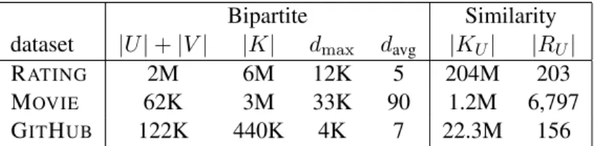
A real-world dataset named ‘rec-eachmovie’[4], whose edge denotes that an audience gives a review of a movie and whose audience side similarity graph has 1.2M edges with 6979 extinct CN weights, is used to illustrate the CN property of real-world streaming bipartite graph. We analyze the distributional properties of CN and plot out the CN weights as the function of dense ranks (Figure1.1 left) and the cumulative fractions as the function of dense ranks (Figure1.1 right). From the left plot of Figure1.1, 6000 out of 6979 dense ranked edge weights are comparatively much larger than the remaining. From the right plot of Figure1.1, 6000 out of 6979 dense ranks contain only 1% of total edges. Combination of the two plots tells us that the high ranked edges which is much larger than the remaining consist only a very small portion of the edge sets, which also means in similarity graph, there is a huge tail of very small weighted edges, which actually could be ignored in analysis. Most real-world bipartite streams, including the other two datasets in this thesis named ‘rec-amazon-rating’ and ‘rec-amazon-rating’, also have the similar features in the distribution of edge weights.
Figure 1.1: Similarity Edge Weight (left) and Cumulative Fraction (right) as function of dense edge rank for ‘rec-eachmovie’ dataset
Based on the property we discussed above, a weighted sampling scheme like Priority Sampling[5] that can select heavier weighted edges with a higher probability is the sam-pling method we should apply to real-world streaming bipartite graph. This thesis aims to provide such a sampling scheme to help us analyze the node similarity in real-world streaming bipartite graph.
1.2 Contribution and Outline
In this thesis, we propose a new single pass scheme to sample the similarity graphs of streaming bipartite graph with fixed storage and to provide unbiased estimates of the CN similarity weights.
We describe the notations and the problems in Section 2. Our algorithm is introduced in Section 3. Our algorithm is based on Priority Sampling which is to keep a reservoir of k highest priorities during the stream and the priority for each item is its weight divided by
1. Bipartite Edge Sampling. We construct a fixed size reservoir for bipartite edge stream. The weights for bipartite edges are determined by minimizing the estima-tion variance of CN weights. We provide two choices for the weights: fixed weight or adapted weight and compare the results.
2. Sample-Based Similarity Aggregation.Each new arriving bipartite edge would cause an update to the CN weights of each similarity edge attached to its nodes. We also construct a fixed size reservoir to sample the edges in similarity graph.
Then the detailed algorithm, data structure and time & space cost would be analyzed in Section 4. In Section 5, we emphasize in the algorithm of SIMADAPT and prove its properties. In Section 6 we evaluate our algorithm using three public bipartite graphs and introduce some additional methods to control error. With 10% sampling rate for both bipartite and similarity edges, the weights of edges with the top-100 dense ranks are es-timated with the weighted relative error of around 10%, and the correlation between true and estimated ranks is over 90%. We review related work in Section 7 and conclude in Section 8.
2. OVERVIEW OF PROBLEM
2.1 Notation of Graph
Let G = (U, V, K) denote a bipartite graph with disjoint node sets U, V and un-weighted and unrepeated edge setK. For each edgee∈ K, it has an end pointu(e) ∈U
and another end pointv(e)∈V. For a subsetS ⊂Kof edges, we denoteU(S) ={u(e) :
e∈S}andV(S) ={v(e) :e∈S}to be the corresponding sets of endpoints in two node sets. N(u) = {v : (u, v) ∈ K} denotes the neighbor set ofuin V and correspondingly
N(U′) =∪u∈U′N(u)forU′ ⊂U. d(w)denotes the degree of any nodew.
LetGU = (U, KU, C)denote the similarity graph ofGonU. The CN weight set isC andC(u, u′) = |N(u)∩N(u′)|. The edge set in similarity graph isKU = (u, u′) :C(u, u′)>0.
In the streaming bipartite graph model, the edgesK arrive in a sequence. Let Kn to denote the first n arriving edges, Gn = (Un, Vn, Kn) to be the sub graph of G, where
Un =U(Kn)andVn =V(Kn), andCnto be the corresponding similarity. 2.2 Problem Description
In this thesis, we address the following problem: for eachn, compute in fixed storage an unbiased estimateCˆnof the similarityCn of the sub graphGnformed from its firstn edges.
3. BIPARTITE GPS FOR SIMILARITY ESTIMATION
Our approach combines two stages of sampling. First, we maintain a sample of edges from the streaming bipartite graph using Graph Priority Sampling with fixed storage. The sampled bipartite edges generate an unbiased estimator of the similarity graph. Second, we employ a further sample based aggregation to accumulate an estimator of similarity graph, also in fixed storage.
3.1 Bipartite Graph Priority Edge Sampling
The essence of our algorithm is from Priority Sampling[5]. It is concluded as follows: For a stream of items with weights ofw0, ..., wn−1, the priority for each item is calcu-lated byri =wi/πi, πi ∈ (0,1]is an independent uniformly distributed random. Priority Sampling maintains a dynamic samplingSof thek < nitems with the highest priority. A thresholdz∗ is the(k+ 1)thpriority. The probability of each sampled item is:
p(k) = min{1, w(k)/z∗} (3.1)
According to the Horvitz-Thompson inverse probability estimator equation, the estimated total weight for each sampled itemi∈Sis:
ˆ
wi =w(k)/p(k) = max(wi, z∗) (3.2)
Fori /∈S,wˆi = 0.
Priority Sampling is extended to be Graph Priority Sampling[6] to count triangles and wedges in graph streams. [6] gives a clear proof of how to choose weight function for graph edge to optimize subgraph variance and presents a scheme of in-stream estimation
which is far more accurate than post-stream estimation.
Algorithm 1 from [6] is the main algorithm of the family of in-stream graph prior-ity sampling with the size of the reservoir m. When a new edge k arrives, procedure GPSESTIMATEis first called to do the in-stream estimation. In [6], they did estimations for triangle and wedge counts. In our problem, we would do the estimate updates for similarity graph edges, then the second stage of sampling for the aggregation of simi-larity edges. Secondly, procedure GPSUPDATEwould be called to do priority sampling. We assume a weight function for edge k asW(k,Kˆ). W(k,Kˆ)could include topology, attributes or any information in the graph, for example in the problem of triangles and wedges counting, it is set to be the number of triangles or wedges that contain edge k in
ˆ
K. In this thesis, we take different weight into account and extend the weight from fixed to be adaptive. The weight function in [6] is only related to edgekand the currently esti-mated graphKˆ. We propose a new adaptive weight which would be changed when edges are streaming over time. Section 3.1.1 would fully discuss the selection of the weight function. Once the weightw(k)is computed, a random parameterπ(k)would be assigned to edgek, so that we could get its priority byr(k) =w(k)/π(k). GPS maintains a priority queue (heap) of m edges. Ifr(k) is smaller than the lowest priority in the heap, edgek
would be discarded. If edgekhas a higher priority, the edge with the lowest priority would be replaced by edgek. The threshold z∗ is always kept as the priority of the(m+ 1)th edge, which would be used to calculate the probability of each edge.
Algorithm 1Family of Graph Priority Sampling Algorithms[6] 1: procedureGPS(m)
2: Kˆ =∅ ▷Bipartite edge sample
3: z∗ = 0 ▷Threshold
4: whilenew edge kdo
5: GPSESTIMATE(k) ▷In-stream estimation
6: GPSMAIN(k, m) ▷Priority sampling
7: end while 8: end procedure 9:
10: procedureGPSESTIMATE(k)
11: In-stream estimation, like count triangle/wedge, or update similarity graph 12: end procedure 13: 14: procedureGPSMAIN(k, m) 15: π(k) =U ni(0,1] 16: w(k) = W(k,Kˆ) 17: r(k) =w(k)/π(k) ▷Priority of edgek 18: p(k) = 1 ▷Probability of edgek 19: Kˆ = ˆK ∪k 20: if|Kˆ| ≤mthen 21: return 22: end if
23: k∗ =argmink′∈Kˆ r(k′) ▷Lowest priority edge
24: z∗ = max{z∗, r(k∗)} ▷New threshold
25: Kˆ = ˆK \ {k∗} ▷Remove lowest priority edge
26: Deleteπ(k∗), w(k∗), r(k∗), p(k∗) 27: end procedure
3.1.1 Edge Weight Function
We now specify the weight function used for edge selection. It was shown in [6], the variance of the estimator of increment of the number of subgraphs caused by the addition of an edge is minimized by using that increment as a weight for priority sampling. Let’s say the total similarity of nodeuis the sum of the similarity of edges connected to nodeu
in similarity graphGU. C(u) = ∑ u′∈U C(u, u′) = ∑ v∈N(u) (|N(v)| −1) (3.3)
When a new edge e = (u, v) comes, it brings a new neighbor nodev to u, so brings an increment of|N(v)| −1toC(u). At the same time, C(v) also increases by|N(u)| − 1. Therefore, the overall similarity that edgeebrings to its endpoints is|N(u)|+|N(v)| −2. To avoid weight of 0, we will assign an edge(u, v)with the weight
w(u, v) =|Nˆ(u)|+|Nˆ(v)| (3.4)
Actually, it is obvious that this kind of weight function is not fair for the early arrived edges compared to late edges. Their weights would be comparatively smaller than the late arrived edges since the degrees of nodes could increase during the stream. So we come up with an idea of incremented weights, which allows edges arriving early in the stream to acquire a greater weight as the topology develops. We also include uniform weight
w(u, v) = 1for comparison as a baseline. We propose two variants of edge weights:
1. Fixed Weights The weight of edge w(u, v) = |Nˆ(u)|+|Nˆ(v)| is determined from the sample edge setKˆ upon arrival and is fixed thereafter.
2. Incremented WeightsThe weight of edgew(u, v)is incremented by 1 for each sub-sequent edge arrival as long as they share the same node, such as e = (u, v′) or
e = (u′, v). The weight of an edge is not correspondingly decremented when ad-joining edges are ejected from the sample. Once the weight of edge is incremented, its priority would also increaser(k) =w(k)/π(k).
3.1.2 In-stream Estimation of Similarity Graph
During the in-stream estimation, we calculate the similarity C between nodes from the same node set. Actually the similarity between node uandu′ is equal to the number of wedges between u and u′, to be denoted as C(u, u′) = {(u, v, u′) : v ∈ N(u) ∩
N(u′)}. Let’s assume Gn is a non-sampled graph, then the number of newly created wedges in similarity graph on U sideGU by edge en = (u, v)is equal to the number of edges that are connected with nodev. ConsiderGnis sampled, so each update should take the form of the Horvitz-Thompson inverse probability estimator, which is like equation 3.5. Correspondingly, the updates that edgeen = (u, v)caused to similarity graph on V sideGV are another series of updates like equation 3.6.
{αn(u, u′) = 1/pn−1,(u′,v) :u′ ∈Nˆn−1(v)} (3.5)
{αn(v, v′) = 1/pn−1,(u,v′) :v′ ∈Nˆn−1(u)} (3.6) As for the probability of each edge has the equation 3.7. Let’s assume the edge weight is fixed, then equation 3.8 guarantee thatzt+1 > zt. Then pt+1(k) < pt(k). Therefore, in Algorithm 2 Procedure BGPSUPDATE(k), which is to update the probability of edgek, is only needed to be called right before p(k)is used in similarity stream, since at that time
p(k)is the minimum value.
p(k) = min{1, wt(k)/zt∗ :tis time sequence throughout the stream} (3.7)
zt+1 = max{zt, r(kt∗)} (3.8) However in the condition of adaptive weight, the weight of the edge could increase, so the probability of the edge should always be updated every time the threshold is increased.
In section 5.1, it is proved that we could simplify this procedure and also update the edge’s probability when a new adjacent edge arrives.
Then, we could estimate the similarity edges by accumulating estimates of updates that are generated by arrivals to the edge reservoir sample Kˆn. Therefore, the GPSES-TIMATE procedure in our algorithm is as below as BGPSESTIMATE. u, v indicates the source and target node of edgek. GU, GV are similarity graphs and are initialized in the main procedure. N(w) denotes neighbors of node w and would be maintained in main procedure.
Algorithm 2In-stream Similarity Updates Without Sampling 1: procedureBGPSESTIMATE(u, v, N(u), N(v), GU, GV)
2: foru′ ∈N(v)do ▷For every other neighbor node ofv
3: BGPSUPDATE((u′, v), z∗) ▷Update the probability of edge(u′, v) 4: ifSimilarity edge(u′, u)∈/ GU then
5: GU =GU ∪(u′, u) 6: end if
7: C(u′, u)+ = 1/p(u′, v) ▷Accumulate similarity 8: end for
9: forv′ ∈N(u)do ▷Same withGV
10: BGPSUPDATE((u, v′), z∗)
11: ifSimilarity edge(v′, v)∈/GV then 12: GV =GV ∪(v′, v) 13: end if 14: C(v′, v)+ = 1/p(u, v′) 15: end for 16: end procedure 17: 18: procedureBGPSUPDATE((k, z∗)) 19: ifz∗ >0then 20: p(k) = min{p(k), w(k)/z∗} 21: end if 22: end procedure
every similarity edge, we use another sample-based approximation to provide unbiased estimates of the aggregates in fixed storage, which is discussed in section 3.2.
3.2 Similarity Stream Aggregation
The sum of similarity stream∑ni=1αi(w, w′)is unbiased estimates of the true similar-ityC(w, w′). However, aggregating these across all sampled node pairs inU orV would require space equal to the cardinality of the edge pair of the sampled similarity graph. Instead we will use a further reservoir sample-based aggregation of the stream of updates
ˆ
α(w, w′). This yields an unbiased estimate of the true similarity in fixed storage. There are several algorithms we could choose from, such as Adaptive Sample & Hold[7], Stream VarOpt[8], Priority Sample and Hold[9]. In this thesis, we implement Priority Sample and Hold (PrSH).
The process of PrSH is very similar to priority sampling. The only difference is the calculation for the estimator. The estimator of weight for keykisXˆkis defined iteratively by equations as below, assuming the arriving key isi, the reservoir sample isKˆ:
ˆ Xk,t = ˆ Xk,t−1+x i∈Kˆt−1 andi=k ˆ Xk,t−1 i∈Kˆt−1 andi̸=k x i /∈Kˆt−1,i∈Kˆtandi=k ˆ Xk,t−1qk,t−1/qk,t i /∈Kˆt−1,i∈Kˆtandi̸=k (3.9)
The algorithm in [9] is shown as Alg.3. At the beginning, AGGREGATE.INITIALIZEis called to create a reservoir of size m. Every time a similarity update is created, AGGRE-GATE.ADDis called to add this update into the similarity stream. When all the process is done, every similarity edge kneeds to be updated for the last time, which means method AGGREGATE.UPDATEALL would be called at the end of the whole algorithm. Then, we
could get the estimators for the weights of similarity edges.
Algorithm 3Similarity Stream Aggregation using PrSH [9] 1: classAGGREGATE 2: methodINITIALIZE(m) 3: K ← ∅;z∗ ←0; size←m 4: end method 5: 6: methodADD(k, α) 7: ifk ∈Kthen 8: U pdate(k) 9: a(k)+ =x;w(k)+ =x 10: return 11: end if 12: K =K ∪ {k}; 13: π(k) =U ni(0,1];w(k) =x;p(k) = 1 14: r(k) = w(k)/π(k) ▷Priority of edgek
15: a(k) = x ▷Estimator of weight of edgek
16: if|K| ≤sizethen
17: return
18: end if
19: k∗ =argmink′∈Kˆ r(k′) 20: z∗ = max{z∗, r(k∗)}
21: Kˆ = ˆK \ {k∗} ▷Remove lowest priority edge
22: Deleteπ(k∗), w(k∗), r(k∗), p(k∗), a(k∗) 23: end method 24: end class 25: 26: methodUPDATE(k) 27: a(k) = a(k)∗q(k) 28: q(k) = min{q(k), w(k)/z∗} 29: a(k) = a(k)/q(k) 30: end method 31: 32: methodUPDATEALL
33: foreach similarity edgek ∈K do 34: AGGREGATE.UPDATE(k) 35: end for
4. ALGORITHMS AND IMPLEMENTATION
4.1 Algorithm Details
In this thesis, we would continue to use the scheme in Algorithm 1. Algorithm 4 is the detailed algorithm to estimate nodes similarities in bipartite graphs with adaptive weight and PrSH second stage sampling. Let’s specify this algorithm as SIMADPAT. The algorithm with fixed weight would just remove the part of INCREASEWEIGHT(line 33), and would be specified as SIMFIXED in the rest of the thesis. The algorithm without second stage sampling would use procedure BGPSESTIMATE in Algorithm 2 instead of BGPSESTIMATEhere.
We focus on the similarity graph on the sourceU side here and omit the same process for target V nodes set. The initialization of sampled bipartite graph and constructed sim-ilarity graph take place (line 2-3). When a new edge(u, v)arrives, procedure BGPSES-TIMATEwould be called to construct similarity graph. In procedure BGPSESTIMATE, the probability of each adjacent edge would be updated first (line 13). Then, similarity graph update is generated and added to the second stage stream (line 14). If no sampling is ap-plied, the inverse probability weight would be added directly to similarityClike line 7 in Algorithm 2.
Algorithm 4In-stream Bipartite GPS with Adaptive Weight and PrSH 1: procedureBGPS(m)
2: Kˆ =∅,z∗ = 0
3: AGGREGATE.INITIALIZE(m) 4: whilenew edge(u, v)do
5: BGPSESTIMATE(u, N(v)) ▷In-stream estimation
6: BGPSMAIN(u, v, m, N) ▷Priority sampling
7: end while
8: AGGREGATE.UPDATEALL
9: end procedure 10:
11: procedureBGPSESTIMATE(u, N(v))
12: foru′ ∈N(v)do ▷For every other neighbor node ofv
13: BGPSUPDATE((u′, v), z∗) ▷Probability update, in Alg.2 14: AGGREGATE.ADD((u, u′),1/p(u′, v)) ▷PrSH sampling 15: end for 16: end procedure 17: 18: procedureBGPSMAIN(u, v, m, N) 19: Kˆ = ˆK ∪k 20: N(u) = N(u)∪ {v},N(v) = N(v)∪ {u} 21: π(u, v) =U ni(0,1],p(k) = 1 22: w(u, v) = |N(u)|+|N(v)| 23: r(u, v) =w(u, v)/π(u, v) 24: if|Kˆ| ≤mthen 25: return 26: end if
27: (u∗, v∗) =argmin(u′,v′)∈Kˆ r(u′, v′) ▷Lowest priority edge 28: z∗ = max{z∗, r(u∗, v∗)} ▷New threshold 29: Kˆ = ˆK \ {(u∗, v∗)} ▷Remove lowest priority edge 30: N(u∗) = N(u∗)\ {v∗},N(v∗) =N(v∗)\ {u∗}
31: Deleteπ(k∗), w(k∗), r(k∗), p(k∗)
32: if(u, v)̸= (u∗, v∗)then ▷In fixed weight, omit the following part 33: INCREASEWEIGHT(u, v, N(u), N(v)) 34: end if 35: end procedure 36: 37: procedureINCREASEWEIGHT(u, v, N(u), N(v)) 38: foru′ ∈N(v)\ {u}do 39: BGPSUPDATE((u′, v), z∗)
40: w(u′, v) + + ▷Increment edge weight
41: end for 42: forv′ ∈N(u)\ {v}do 43: BGPSUPDATE((u, v′), z∗) 44: w(u, v′) + + 45: end for 46: end procedure
Procedure BGPSMAINconcerns updating the bipartite edge sample. Edges are main-tained in a priority queueK based on increasing order of edge priority. When a new edge arrives, the edge is inserted into the sample reservoir (line 19-20) first. This part happens before the weight assignment to avoid the edge weight to be zero. Then the priority of each(u, v)is computed as the quotient of the edge weightw(u, v)(the sum of the degrees ofuandv) and a permanent random number in (0,1]. If there are fewer than or equal to
medges in the current graph sample, just return. Otherwise, the edge of minimum prior-ity is deleted (line 29-31). In SIMADAPT, the INCREASEWEIGHTprocedure updates the probability of all adjacent edge first, then increments the weight of all adjacent edge to reflect the increased degree of their endpoints (line 40). This change may require updating in their position in the priority queue.
4.2 Data Structure and Time Cost
Aminimum heap is used to implement priority queue, where the root position is the edge with the lowest priority. Therefore, access to the lowest priority edge is performed in
O(1). Insertions areO(logm)worst case.
However,heapis not a friendly structure for search, which takesO(m)in average. In SIMADAPT, each insertion of an edge(u, v)increments the weights of its|N(u)|+|N(v)| neighboring edges. Each weight increment may change its edge’s priority, requiring its position in the priority queue could be found out easily. So we use another map to store the position of each item. When items in heap shift up or down, their positions information in map also swap. Therefore, the complexity of search is reduced toO(1)and edge updates becomesO(logm). While the worst case cost for the binary heap update isO(logm), the average cost is O(1). Since the priority is incremented, an edge may be bubbled down by exchanging with its lowest priority child if that has lower priority. Assuming uniform distribution of initial position, the average cost isO(m−1∑log2m
h=0 2 h(log
where the sum is over levelshin the binary heap. 4.3 Space Cost
For SIMADAPT and SIMFIXED, we keep two reservoirs for two stages of sampling and each of them has a space cost of O(m) and O(n), m is the edge reservoir capacity and n the similarity reservoir capacity. Besides, we create two map structures to store the neighbors of each node and they cost O(|Uˆ|) andO(|Vˆ|), |Uˆ| andVˆ are the number of nodes in the edge reservoir. The overall space requirement isO(|Uˆ|+|Vˆ|+m+n). Actually, it is a trade-off between time and space. While we can abandon the neighbors map and limit space cost to O(m +n), a pass over the reservoir is required to get the degrees of endpoints, which would be O(m) in time cost. But if we maintain the neighbors map and increase the space, we can achieve sub-linear time for edge updates.
For algorithms without second stage sampling, the size of their similarity graphs are not under our control, which could beO(|Uˆ|2)andO(|Vˆ|2)in worst cases. So their overall space cost would beO(|Uˆ|+|Vˆ|+|Uˆ|2+|Vˆ|2) =O(|Uˆ|2+|Vˆ|2).
5. PROPERTIES AND PROOFS OF SIMADAPT
5.1 Deferred Estimate Update
When implementing SIMADAPTas just described in Algorithm 4, we face a challenge in updating the probability of edge in an efficient way. Since we assume the edges are unique, we could identify them with their arrival orderi∈ [|K|]. The probability thatiis in the sample at timet,t ≥iis:
pi,t =P[i∈Kˆt] =P[ri,s > zs:s∈[i, t]] =P[πi ≤wi,s/zs :s∈[i, t]] =P[πi ≤ min s∈[i,t]wi,s/zs] = min{1,min s∈[i,t]wi,s/zs} = min{pi,t−1, wi,t/zt}
(5.1)
Therefore, in principle it is necessary to updatepi,t for eachiand whent≥i. For SIMFIXED, this turns out not necessary sincewi,t =wi, then:
pi,t = min{1,min
s∈[i,t]wi/zs} = min{1, wi/max
s∈[i,t]zs}
(5.2)
probability becomes in SIMFIXED:
pi,t = min{1, wi/z∗t} (5.3)
For SIMADAPT, the weight of edgeiwould be incremented step by step. For timet, letβi,tbe the earliest timesat whichwi,sheld its current value, i.e.,
βi,t = min{s≤t:wi,s=wi,t} (5.4)
Assuming γi,t is the latest times at which wi,s will hold its current value, which means afterγi,t, the weight of edge is incremented by 1, i.e.,
γi,t = max{s≥t:wi,s=wi,t} (5.5)
wi,γi,t+1 =wi,t+ 1 (5.6)
We claim the following method ofdeferred updatesgets the same probability through-out the stream with equation 5.1.
Deferred Updates:Every time when the weight of edgeiis about to increment, update its probability, i.e.,
qi,γi,t = min{qi,βi,t−1, wi,γi,t/z
∗
γi,t} (5.7)
Then at timeβi,t ≤t ≤γi,t, probability of edgeiis:
qi,t = min{qi,βi,t−1, wi,t/z
∗
t} (5.8)
Proof. We would prove in iteration. Let’s assumeqi,βi,t−1 = pi,βi,t−1, and to proveqi,t = pi,t.
Whenβi,t ≤t ≤γi,t, its probability meets the equation of 5.9. Since the weight during this time stays the same, so it becomes the equation of 5.10.
pi,t = min{pi,βi,t−1, min
s∈[βi,t,t]
wi,s/zs} = min{qi,βi,t−1, min
s∈[βi,t,t]
wi,s/zs}
(5.9)
pi,t = min{qi,βi,t−1, wi,t/ max
s∈[βi,t,t]
zs} (5.10)
We know thatz∗t ≥maxs∈[βi,t,t]zs. In the case ofz
∗
t = maxs∈[βi,t,t]zs, we have: pi,t = min{qi,βi,t−1, wi,t/z
∗
t}=qi,t (5.11)
In the case ofzt∗ >maxs∈[βi,t,t]zs, thenz
∗
t =zβ∗i,t−1, then we have: wi,t maxs∈[βi,t,t]zs > wi,t zt∗ = wi,t zβ∗ i,t−1 > wi,βi,t−1 zβ∗ i,t−1 (5.12)
Ifqi,βi,t−1iteratively updates from the former probability by equation 5.8, then we have: wi,βi,t−1
zβ∗ i,t−1
≥qi,βi,t−1 (5.13)
Therefore, the result of equation 5.10 ispi,t =qi,βi,t−1.
In both of the conditions, we all getpi,t = min{qi,βi,t−1, wi,t/z
∗
t} = qi,t. Therefore, in SIMADAPT, the minimum probability of the edge could be maintained by updates right before the increments of its weight.
5.2 Unbiased Estimation
In this section, we establish that the similarity estimators of SIMADAPTare unbiased, i.e., for eachn, the similarity estimatorCˆnproduced by the firstn arrivals is an unbiased
estimator of the true similarityCnof the graph formed by these arrivals.
The proof is accomplished in three stages. First, we establish unbiasedness of estima-tors of edge counts arising from an algorithm for general time-dependent weights that is similar to SIMADAPT with general weights. Second, we establish that these algorithms coincide the case of nondecreasing weights, which includes the weights of SIMADAPTas a special case. Finally, we show that the similarity estimatorsCˆncan be written as a sum of edge count estimators, whose expectation is the true wedge countCn.
The edge indicator Si,t which take the value 1 if t ≥ i and 0 otherwise indicates whether each i has arrived by timet. We will construct unbiased edge estimators Sˆi,t which are nonnegative random variables that E[ ˆSi,t] = Si,t. Thus by linearity, for any
J ⊂[|K|],SJ,t=
∑
i∈JSi,t will be an unbiased estimator of the number of edges inJ that have arrived by timet. Let Kˆt′ denote the edge reservoir after edget has been processed but before the smallest priority edge is removed, and Kˆt denote the edge reservoir right after the smallest priority edge is removed. Therefore,zt = mini∈Kˆt′ri,t.
Theorem 1. Sˆi,t =I(i∈Kˆt)/qi,t is an unbiased estimator ofSi,t
Proof. When t ≥ i, from the proof in section 5.1, we know that our probability qi,t is exactly equal to the true probabilitypi,tfor anyiandt, i.e.,
qi,t =pi,t =P[i∈Kˆt] (5.14)
ThenE[I(i∈Kˆt)] = 1∗P[i∈KˆT] + 0∗P[i /∈Kˆt] =P[i∈Kˆt] =qi,t, we have:
E[ ˆSi,t] =E[I(i∈Kˆt)]/qi,t = 1 =Si,t (5.15)
of the exact similarityCn from the truncated streamKn. Each arriving eachen = (u, v) contributes toC(u,′u)through wedges (u, v, u′)forv ∈ N(u)∩N(v). Thus to compute
C(u, u′)we count the number of such wedges occurring up to timen, i.e.,
Cn(u, u′) = n ∑ i=1 ∑ v∈N(u)∩N(u′) ( I(u(ei) =u))Si−1,(u′,v) +I(u(ei) =u′))Si−1,(u,v) )
We replace theSi−1,(u,v)by their estimates Sˆi−1,(u,v) and, by linearity, obtain an unbi-ased estimate ofCn. ˆ Cn(u, u′) = n ∑ i=1 ∑ v∈N(u)∩N(u′) ( I(u(ei) =u)) ˆSi−1,(u′,v) +I(u(ei) =u′)) ˆSi−1,(u,v) )
6. EXPERIMENTS AND EVALUATIONS
Our experiments use three datasets comprising bipartite graphs drawn from real-world applications, and they are publicly available at Network Repository [4]. Their basic prop-erties are listed in Table 6.1. In the bipartite graphG= (U, V, K),|U|+|V|is the number of nodes in both partitions,|K|is the number of edges,dmaxthe maximum degree anddavg the average degree. |KU|is the number of edges on the source side of the similarity graph and|RU|the number of dense ranks, i.e. the number of distinct weight values.
1. RATING: the datasetrec-amazon-ratings. The source vertex is an Amazon user and the target vertex is an Amazon product. An edge denotes that a user rated a product. There are2,146,058users,1,230,917products, and5,838,043ratings.
2. MOVIE: the datasetrec-each-movie. The source vertex is an audience member and a target vertex is a movie. An edge denotes that an audience gives a review of a movie. There are overall1,623 audience members,61,265movies and2,811,717 reviews. The maximum and average node degrees are both much larger than the other two datasets.
3. GITHUB: the datasetrec-github. The source vertex is a GitHub user and the target vertex is a GitHub project. An edge denotes that a user is a member of a project.
Bipartite Similarity
dataset |U|+|V| |K| dmax davg |KU| |RU|
RATING 2M 6M 12K 5 204M 203
MOVIE 62K 3M 33K 90 1.2M 6,797
GITHUB 122K 440K 4K 7 22.3M 156
Table 6.1: Datasets and characteristics. Bipartite graph: |U|+|V|:#nodes,|K|: #edges,
There are56,519users,120,867projects and440,237membership relations. In this paper, we report experimental results concerning estimation of the similarities of pairs of source nodes in the graph.
Finally, for these experiments, we used a 64-bit desktop equipped with an Intel˝o Core i7 Processor with 4 cores running at 3.6 GHz.
6.1 Accuracy Metrics
Since applications such as recommendation systems rank recommendation based on similarity, our metrics focus on accuracy in determining higher similarities that dominate recommendations, and exploit in part metrics that have been used in the literature; see e.g., [10].
6.1.1 Weighted Relative Error.
A standard measure of the accuracy of a point estimateCˆ(e)relative to the true value
C(e)for a single similarity edgee, is the relative errorRE(e) =|Cˆ(e)−C(e)|/C(e). For ranking applications, there is greater interest in the accuracy of higher weight edges. For this reason, we summarize the set of relative errors with an average that is weighted by the true edge weight. Specifically, for eachk we compute the top-k dense rankedweighted relative error. WRE(k) = ∑ e∈KˆU,k |Cˆ(e)−C(e)| C(e) C(e) ∑ e∈KˆU,kC(e) = ∑ e∈KˆU,k| ˆ C(e)−C(e)| ∑ e∈KˆU,kC(e) (6.1)
6.1.2 Dense Rankings and their Correlation.
dense ranking, in which edges with the same weight values have the same rank, and ranks are consecutive. Dense ranking is insensitive to random permutations of equal weight edges and reduces estimation noise.
To assess the linear relationship between the true and estimated ranks we use Spear-man’s rank correlation on top-kestimated ranks. For each similarity edgeein the sampled similarity graphGˆU, letreandrˆedenote dense ranks ofC(e)and⌊Cˆ(e)⌋respectively. The top-krank correlation over pairs{(re,rˆe) :e ∈KˆU,k}withKˆU,k={e∈Kˆk : ˆre ≤k}is
Cor(k) = Cov(r,rˆ)/√Var(r)Var(ˆr) (6.2)
6.1.3 Precision and Recall.
We evaluate accuracy of rank prediction using prediction and recall for top-k dense ranks: Prec(k) = KUk∩KˆU,k ˆ KU,k , Rec(k) = KUk ∩KˆU,k KU,k (6.3) A standard summary ranking statistic from applications in Recommender Systems is the Area under the Recall curve ATOP [11], defined up to rankkas
ATOP(k) = 1 k k ∑ i=1 Rec(i) (6.4) 6.2 Experiment Description 6.2.1 Data Preparation
The datasets were originally presented in source node order. We rearranged edges in a random order and eliminated any duplicate edges.
6.2.2 Sampling Rates
We applied the SIMADAPTand SIMFIXEDto each dataset, with the edge sample reser-voir sizemequal to fractionsfm of the total bipartite edges, and the second stage sample aggregation reservoir sizenequal to fractionsfnof the cardinality of the actual projection graph without sampling.
For the first stage, sampling fractions were fm ∈ [5%,10%,15%,20%,25%,30%]. The second stage sampling fractions werefn∈[5%,10%,15%,100%], where 100% reser-voir means aggregation without sampling was used in the second stage.
6.2.3 Error Control
We use two forms of noise reduction that can be regarded as an enhancement to the algorithm. The first form is simple averaging. We ran five separate instances of the al-gorithm on each data stream (with the same randomized input data) and averaged the resulting similarity estimates.
The second form of error control method is filtering by update count, which comprises eliminating all similarity edges for which the number of updates is less than a specified threshold. The motivation here is estimates comprising a small number of updates may be subject to relatively large noise due to the1/pform of the inverse probability estimators, which means a single extremely small p could result in huge similarity weight. In other words, we would like to remain the heavy similarity edges due to large numbers of updates but not due to few times extreme random updates. On the other hand, estimates with a larger count benefit more from statistical averaging.
In our experiments, we explored the benefits of threshold filter counts of [1,5,10,15] and 0 (i.e., no filtering). We note that filtering incurs an implementation cost of maintain-ing an additional counter per aggregate.
6.3 Experiment Results
In this section we report results concerning the error/accuracy metrics described above (WRE,Cor,Prec,Rec, ATOP) for the different algorithms (SIMFIXED and SIMADAPT) across a range of edge and similarity sampling rates, applied with various filter thresholds to the three datasets (RATING, MOVIE, GITHUB). Firstly, we narrow the scope of explo-ration of these parameters by establishing common filtering thresholds across the datasets. Then we study the effect of second stage similarity sampling and find out the ideal sam-pling rate. Next, we apply this count filters and PrSH rate to all the experiments and compared the results from different algorithms (SIMFIXED and SIMADAPT). In the end, we compare the results of our algorithms with other methods, including simple uniform sampling and common neighbors method in [12].
6.3.1 Filtering Analysis
We would first discuss the effect of count filters in data analysis. Figure 6.1 gives you a straightforward understanding how a filter works here.
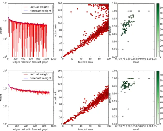
Figure 6.1: Error reduction with filtering. Top: no filtering. Bottom: count filter 10. Dataset GITHUB, Alg. SIMADAPT, edge sample 10%, no PrSH, top 100 dense ranks
Figure 6.1 is experiment result from GITHUBdataset with SIMADAPTalgorithm. The top three plots are original similarity graph data without filtering and the bottom three plots are results after filtering with the count filter of 10. We selected the top 100 dense ranked edges from forecast graph and found out their true weight and rank in actual graph.
The left column displays the comparison of actual and forecast weight of these approx-imately 1000 edges. The reduced number of edges in bottom plot reflects the number of filtered out edges. With no filtering, the noise in the actual weight curve corresponds to a relatively small proportion of similarity edges whose estimated weight greatly exceeds the true weight due to estimation noise. The count filter deleted most of those edges with over exaggerated weight in forecast graph.
The middle column shows a scatter plot of the actual vs. forecast dense ranks for the same edges. It shows clearly that the edges with both top ranks in the forecast and actual graphs were not affected by the filtering, but a cluster of edges with top forecast rank but lower true rank (i.e. lower true weight) are removed by filtering.
The right column shows a scatter of precision vs. recall for top-n queries forn from 1to100, where the color density of points increases withn. Note how filtering improves precision.
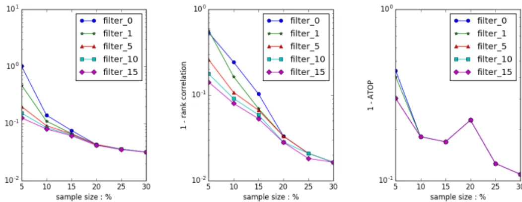
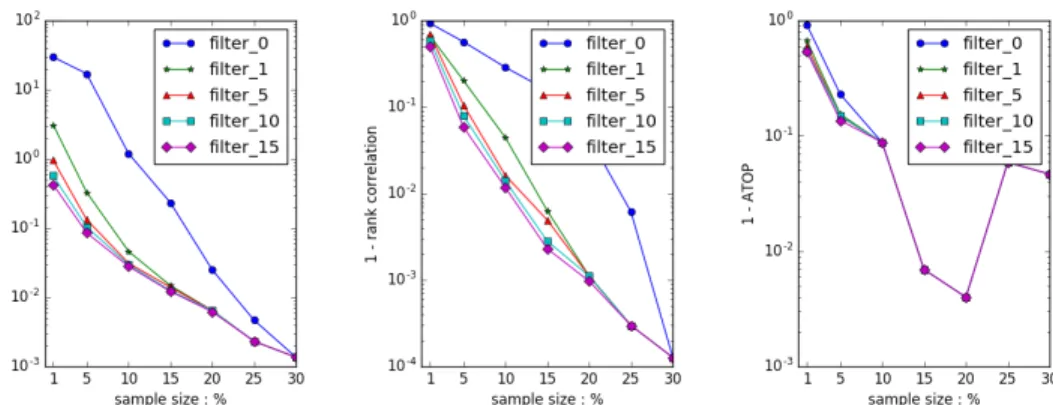
Back to the metrics we introduced above, we plot Figure 6.2, which displays WRE (left), Cor (center) and ATOP (right). In order to make lines in three plots with consis-tent order, we plots (1−Cor) and(1−ATOP)in center and right figures. Similarly to SIMADAPT count filtering also works well in SIMFIXED. We analyze the top 100 edges from the same dataset GITHUB without PrSH, but with SIMFIXED algorithm. From left and center plots, we could see that filtering can provide magnitude reduction in WRE and (1−Cor)across sampling rates smaller than 20%. When the probability is larger or equal to 20%, the precisions of estimations without filter have already been very high, so we could not see big differences in top 100 edges. However, when we enlarge the analysis set to be top 150 dense ranked edges, count filters bring significant improvement all across the sampling rates, which is shown in Figure 6.3.
Figure 6.2: Error reduction with filtering. Dataset GITHUB, Alg. SIMFIXED, no PrSH, top 100 dense ranks
Figure 6.3: Error reduction with filtering. Dataset GITHUB, Alg. SIMFIXED, no PrSH, top 150 dense ranks
We got the similar results with dataset MOVIE and RATING. The results of RATING are shown in Figure 6.4. Sum up the results of three datasets with several algorithms, we found that filtering at a value of 10 to be most effective. Since there is no cost in accuracy in setting the threshold beyond the point of “diminishing returns” we recommend and adopt a filtering threshold of 10. All the results in the rest of thesis are applied with a filter
of 10 except special notations.
Figure 6.4: Error reduction with filtering. Dataset RATING, Alg. SIMADAPT, no PrSH, top 150 dense ranks
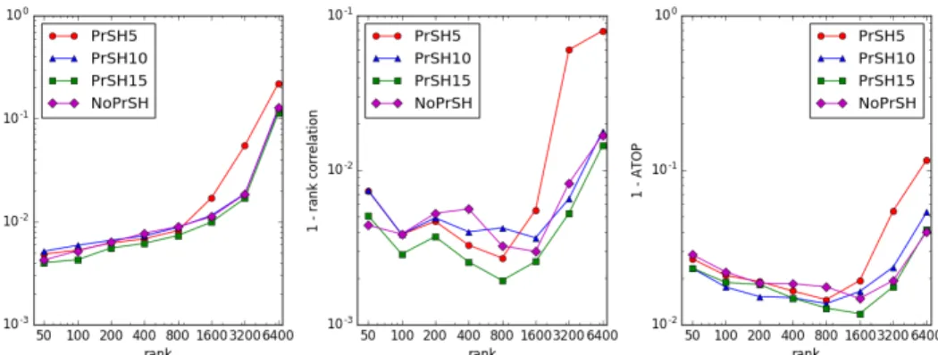
6.3.2 Second Stage PrSH Sampling
In all our datasets we found that PrSH second stage has little effect in accuracy for sampling rates down to about 10% (and less in some cases) under a wide variety of con-ditions. This is illustrated in Figure 6.5 for the example of MOVIEfor SIMFIXEDat edge sampling fractionfm = 10%and PrSH sampling rates of 5%, 10%,15% and 100%(i.e. no PrSH sampling), which displays error matrics for edges with the top-k dense ranks, as a function ofk. Forkup to several hundred, even 5% PrSH sampling has little or no effect, while errors roughly double when all ranks are included.
Figure 6.5: Second Stage Sampling with PrSH at 5%, 10%, 15% and none, as function of topnranks. Dataset MOVIE, Alg. SIMFIXED, 10% edge sampling
Figure 6.6: Second Stage Sampling with PrSH at 5%, 10%, 15% and none, as function of topnranks. Dataset MOVIE, Alg. SIMFIXED, 30% edge sampling
However, when we increase the first stage sampling rate, the performance difference between sampling rates occurs at a much lower rank, just as shown in Figure 6.6. When the edge sampling fraction isfm = 30%, the performance of PrSH5 becomes much worse than others at rank 200, which happened at rank 1600 when fm = 10%. It reveals the fact that when second stage sampling is involved, the larger edge sampling rate could not
guarantee better performance as usual. A large first stage sampling with a small PrSH sampling may perform worse than a small first stage sampling. Figure 6.7 shows this feature clearly with MOVIEdataset and top 800 dense ranked edges. As the edge sampling rate increases larger than 15%, the error metrics for algorithms with PrSH process become larger while error metrics for those without PrSH process are still going down as usual. We also observed similar behaviors in other two datasets, such as GITHUB with top 150 dense ranks in Figure 6.8.
Figure 6.7: Effect of Second Stage Sampling. Dataset MOVIE, top 800 dense ranks
Therefore, our strategy for choosing PrSH sampling rate is when the rank of esti-mated edges is comparatively low, we choose a smaller first stage sampling fraction with a smaller PrSH sampling rate, oppositely when the rank of estimated edges is higher, we choose a larger first stage sampling fraction with a larger PrSH sampling rate.
6.3.3 Different Weights Functions
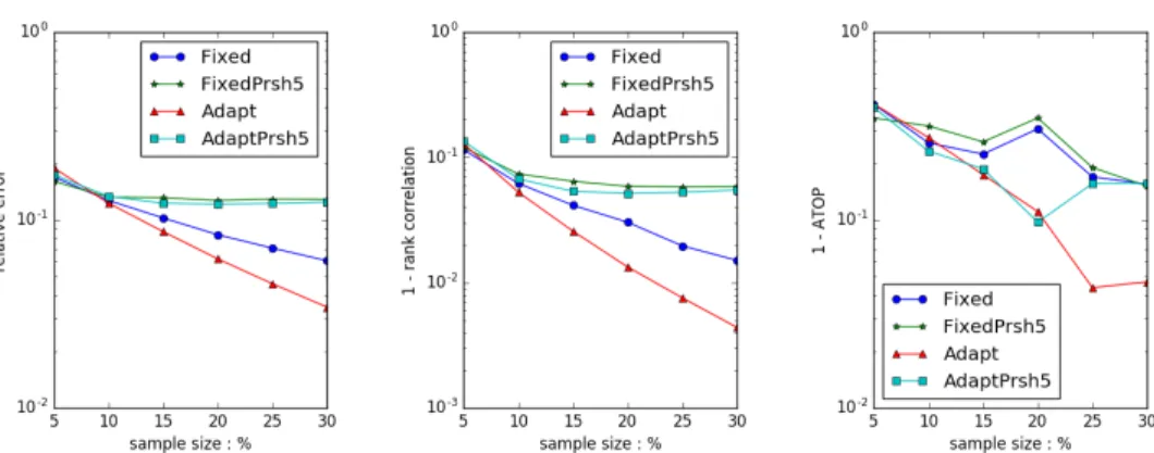
6.3.3.1 Adaptive and Fixed Weights
We now examine the accuracy benefits of SIMADAPT as compare with SIMFIXED. We illustrate these differences in Figure 6.9 for the MOVIE dataset using top 100 dense estimated rank. Each of these figures includes four conditions: SIMADAPTwithout second stage sampling (i.e. 100% sampling rate in PrSH), SIMADAPT with 5% second stage sampling with PrSH, SIMFIXED without and with 5% PrSH. We could notice that two SIMADAPTlines are below the lines of SIMFIXEDacross the sample sizes in all the plots, which means the benefits of adaptive weights are really large compared to the benefits of no sampling in the second stage. When the edge sample ratefm is extremely small at 1%, the results of these four algorithms are similar. With the increase of the first stage sample fraction, the benefits of adaptive weight are enlarged.
Figure 6.9: Algorithm Comparison. SIMADAPT& SIMFIXEDwithout PrSH and with 5% PrSH. Dataset MOVIE, top 100 dense ranks
Similar benefits of SIMADAPTalgorithm is also shown clearly in other two datasets in Figure 6.10 and Figure 6.11. Therefore, we could conclude that the adaptive weight algorithm did a much more accurate estimation than fixed weight algorithm no matter whether the second stage sampling is applied or not.
Figure 6.10: Algorithm Comparison. SIMADAPT & SIMFIXED without PrSH and with 5% PrSH. Dataset GITHUB, top 100 dense ranks
Figure 6.11: Algorithm Comparison. SIMADAPT & SIMFIXED without PrSH and with 5% PrSH. Dataset RATING, top 100 dense ranks
6.3.3.2 Adaptive, Fixed and Uniform Weights
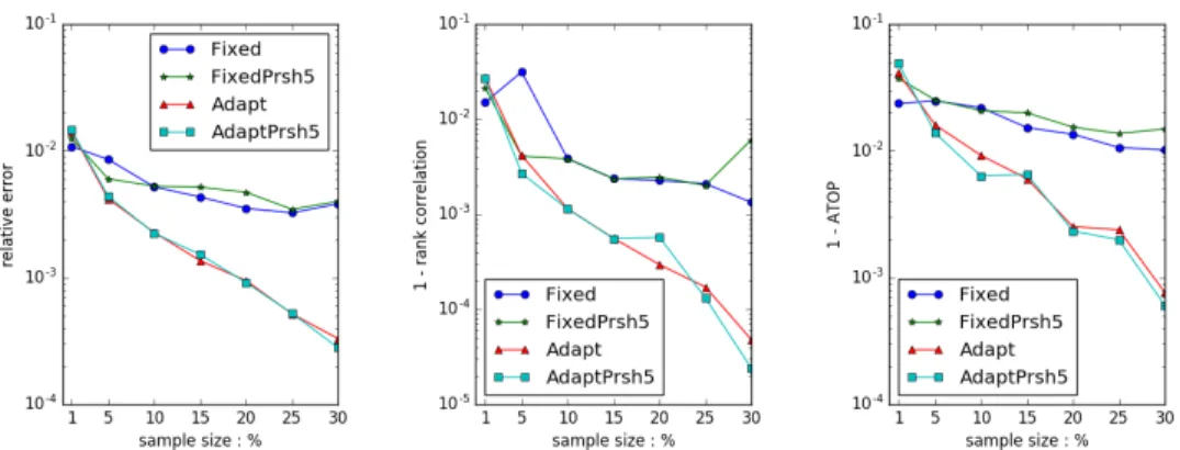
Now, we add another uniform weight function. We change the weight in our algorithm to be 1 for all bipartite edges regardless of their nodes degrees, which means all bipartite edges have the same probability to be sampled. We just need to change line 22 in Algo-rithm 4 to be w(u, v) = 1. This is a baseline to see the effect of our weighted sampling process in SIMADAPTand SIMFIXED.
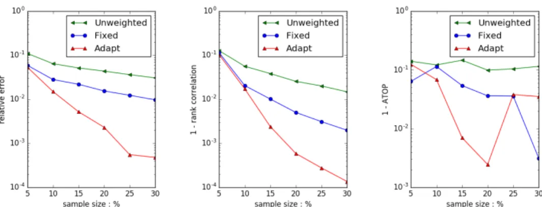
Figure 6.12 and Figure 6.13 are the comparison results of dataset RATINGwithout sec-ond stage sampling and with PrSH rate equal to 5%. ‘Unweighted’ in these plots indicates the condition of the in-stream scheme with uniform weight. Compared to ‘Unweighted’, SIMFIXED shows a little bit improvement but SIMADAPT shows great improvement in error metrics.
Figure 6.12: Algorithm Comparison. Unweighted, SIMFIXED, SIMADAPTwithout PrSH. Dataset RATING, top 100 dense ranks
Figure 6.13: Algorithm Comparison. Unweighted, SIMFIXED, SIMADAPT with PrSH 5%. Dataset RATING, top 100 dense ranks
6.3.4 Comparison with Other Methods
6.3.4.1 Simple Uniform Sampling
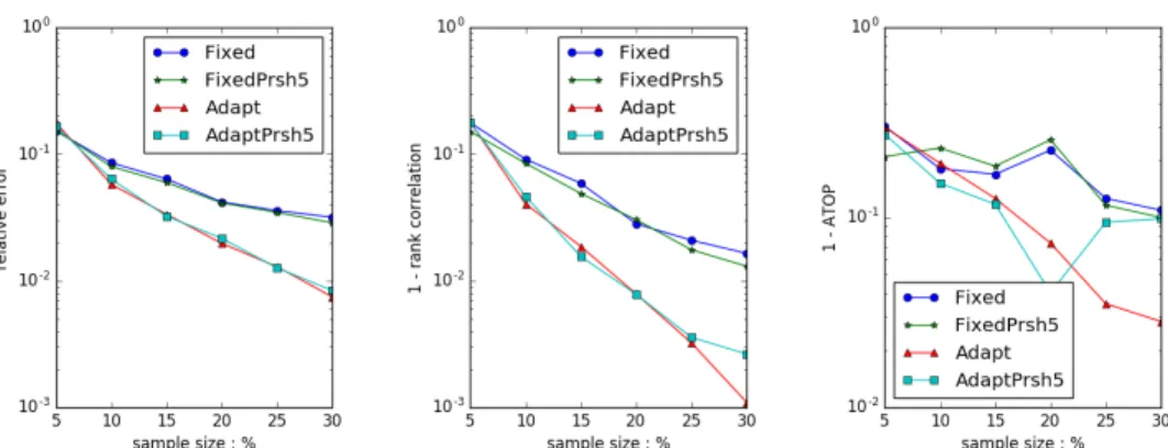
Simple uniform sampling is designed as adopting the most simple uniform edge sam-pling at the same fractions of fm = [5%,10%,15%,20%,25%,30%] at first stage, then constructing similarity graphs according to these sampled edges, during which every sim-ilarity update has the weight ofw(u, u′) = 1/(p(u, v)∗p(u′, v) = 1/(fm)2. It is used as a baseline to show the benefits of our overall scheme, including priority sampling, in-stream similarity updates, count filters etc.
Figure 6.14 and 6.15 illustrates the results of simple uniform sampling with our SIMADAPT and SIMFIXED. They are results from different datasets and different dense ranks, but they all show that both the WRE and rank correlation have a great improvement in our algorithm. ‘Unweighted’ (our algorithm with edge weight equal to 1) is also included to reflect the advantage of the in-stream scheme. Both of ‘Uniform’ and ‘Unweighted’ are unweighted sampling, but with the in-stream scheme, ‘Unweighted’ performs much better.
Figure 6.14: Algorithm Comparison. Uniform Sampling, Unweighted, SIMFIXED & SIMADAPT. Dataset GITHUB, top 50 dense ranks
Figure 6.15: Algorithm Comparison. Uniform Sampling, Unweighted, SIMFIXED & SIMADAPT. Dataset MOVIE, top 200 dense ranks
6.3.4.2 Common Neighbors Method
Sampling for link prediction in non-bipartite graph streams has been proposed in [12]. That work used a separate reservoir of edges for each graph node, with hashing to coordi-nate sampling across different reservoirs to promote selection of common neighbors, and
the setting and applications are different to ours, there are very few papers and algorithms that we could choose from to deal with a streaming graph data. Therefore we did an exper-imental comparison with common neighbors method in [12]. And the detailed algorithm in [12] is as Alg. 5. To reduce the space for random variable of vertexv ∈V, they create a random hash functionG:v ∈V →(0,1).
Algorithm 5Vertex-biased Sampling Graph Sketches [12] 1: procedureCOMMONNEIGHBORS(L)
2: forvertexu∈Gdo
3: η¯(u) =η(u) = 1, S(u) =∅ ▷Initialization 4: end for
5: end procedure
6: fora new edge(u, v)∈Gdo ▷Sampling Process
7: ifv /∈S(u)then 8: if|S(u)|< Lthen 9: S(u) =S(u)∪ {v}
10: else
11: ifG(v)≤η(u)then
12: k ←arg maxw∈S(u)G(w) 13: S(u)←S(u)\ {k}
14: S(u)←S(u)∪ {v} 15: η¯(u)← G(k)
16: k∗ ←arg maxw∈S(u)G(w) 17: η(u)← G(k∗)
18: end if
19: end if 20: end if 21: end for
22: forany node pair(u, u′)inS do ▷Construct Similarity Graph 23: η(u) = (¯η(u) +η(u))/2
24: η(u′) = (¯η(u′) +η(u′))/2 25: C(u, v) = maxS(u){η(u),η(u∩S(u′)′)} 26: end for
fm 5% 10% 15% 20% 25% 30%
MOVIE 864 1730 2596 3463 4329 5195
GITHUB 2 6 10 14 17 21
Table 6.2: Values of L in Alg. Common Neighbors in datasets MOVIE and GITHUB corresponding to edge sampling ratesfm
results with the same space cost. For example, in our algorithm, the overall space cost for edge sampling is 10m = 10fmMb, where m is the size of the edge reservoir, Mb is the total number of edges in the bipartite graph. In COMMONNEIGHBORSprocedure, the space cost is Nu(L+ 2), Nu is the number of nodes in source side. To make them equal, we have: 10fmMb =Nu(L+ 2) L= 10fmMb Nu −2 (6.5)
LetMb andNu to be the exact numbers in each datasets, we calculated the correspond-ingLfor eachfm in[5%,10%,15%,20%,25%,30%]in Table 6.2.
The comparison results are in Figure 6.16 and Figure 6.17. In dataset GITHUB, WRE improves a little bit compared to Uniform Sampling but rank correlation is worse than Uni-form Sampling. And all metrics are much worse than our algorithms. In dataset MOVIE, all metrics are worse than Uniform Sampling and our algorithms.
Figure 6.16: Algorithm Comparison. Common Neighbors, Uniform Sampling, SIMFIXED & SIMADAPT. Dataset GITHUB, top 100 dense ranks
Figure 6.17: Algorithm Comparison. Common Neighbors, Uniform Sampling, SIMFIXED & SIMADAPT. Dataset MOVIE, top 400 dense ranks
I think the reason of the bad performance of Common Neighbors Alg. is it is very average among its nodes that it treats all nodes the same and could not reflect the huge degree differences between them in the real-world data. It may be not suitable for the application of top similarities. And another reason is that many of the reservoirs actually are not full so that the actual space cost of Common Neighbors are much smaller than the
fm 5% 10% 15% 20% 25% 30%
L 864 1730 2596 3463 4329 5195
Actual/Theoretic 0.51 0.39 0.32 0.27 0.24 0.22
Table 6.3: Actual space cost in Alg. Common Neighbors in dataset MOVIE
fm 5% 10% 15% 20% 25% 30%
L 2 6 10 14 17 21
Actual/Theoretic 0.79 0.47 0.36 0.30 0.26 0.23
Table 6.4: Actual space cost in Alg. Common Neighbors in dataset GITHUB
theoretic space cost. In other words, Common Neighbors Alg. has little control on its space consumption. The proportions of actual space cost to theoretic space cost are shown in Table 6.3 and Table 6.4, which is only from 0.22 to 0.79.
7. RELATED WORKS
Bipartite graphs. Recently a number of problems specific to bipartite graphs have attracted attention in the streaming or semi-streaming context. The classic problem of bipartite matching has been considered for semi-streaming [13] and streaming [14] data. Another popular problem in bipartite graph is link prediction [15], which is applied in many areas such as social networks analysis [16], recommendation system [17], or side effect prediction [18]. However few of them could enlarge their dataset to be in the form of data stream.
Graph streams. In the last few years, great interest has been raised in processing large graphs in the model of data stream, which is motivated by the fact that the massive dynamic graphs in the real world could not fit in any main memory or disks of a single ma-chine. [19] concludes all the popular problems and promising research directions in graph streams, which includes connectivity properties, graph distances, approximate matching, frequencies of subgraphs etc. Challenges in graph streams mainly come from the trade-off between time and space cost and the accuracy of online approximate estimation.
Top k queries. The problem of identifying top-k queries in graphs streams has been studied in [20],[21]. The Incremental Threshold (IT) algorithm [22] was the first one to in-troduce continuous top-k queries with sliding information expiration windows to account for information recency. Many other algorithms such as Adaptive spatial-textual Parti-tion Trees [23] were developed later to efficiently serve spatial-keyword subscripParti-tions in location-aware publish/subscribe applications.
8. CONCLUSION
This thesis has proposed a sample-based approach to estimating the similarity (or pro-jection graph) induced by a bipartite edge stream. The statistical properties of real-world bipartite graphs provide an opportunity for weighted sampling that devotes resources to nodes with high similarity edges in the projected graph.
Our proposed algorithms SIMADAPT and SIMFIXED provide unbiased estimates of similarity graph edges in fixed storage, that in evaluation incurs weighted relative errors as low as10%with rank correlation larger than 90% in a10%edge sample. Our algorithms are also compared with others to show their great advantages in weight and rank accuracy. In future work we plan to explore other instances of our framework with edge weights tunes to optimize estimation of other neighborhood based similarity metrics and their ap-plications.
REFERENCES
[1] Zephoria, “The top 20 valuable facebook statistics.” https://zephoria.com/top-15-valuable-facebook-statistics/, 2017.
[2] O. Allali, C. Magnien, and M. Latapy, “Link prediction in bipartite graphs using in-ternal links and weighted projection,” in2011 IEEE Conference on Computer Com-munications Workshops (INFOCOM WKSHPS), pp. 936–941, April 2011.
[3] M. Gao, L. Chen, B. Li, Y. Li, W. Liu, and Y. cheng Xu, “Projection-based link prediction in a bipartite network,”Information Sciences, vol. 376, no. Supplement C, pp. 158 – 171, 2017.
[4] “Datasets of recommendation networks.” http://networkrepository.com/rec.php. [5] N. Duffield, C. Lund, and M. Thorup, “Priority sampling for estimation of arbitrary
subset sums,”J. ACM, vol. 54, Dec. 2007.
[6] N. K. Ahmed, N. Duffield, T. Willke, and R. A. Rossi, “On sampling from massive graph streams,”arXiv preprint arXiv:1703.02625, 2017.
[7] E. Cohen, “Stream sampling for frequency cap statistics,” CoRR, vol. abs/1502.05955, 2015.
[8] E. Cohen, N. Duffield, H. Kaplan, C. Lund, and M. Thorup, “Composable, scalable, and accurate weight summarization of unaggregated data sets,”Proc. VLDB Endow., vol. 2, pp. 431–442, Aug. 2009.
[9] N. Duffield, Y. Xu, L. Xia, N. Ahmed, and M. Yu, “Stream aggregation through order sampling,”arXiv preprint arXiv:1703.02693, 2017.
recom-[11] H. Steck, “Evaluation of recommendations: Rating-prediction and ranking,” inProc. RecSys ’13, (New York, NY, USA), pp. 213–220, 2013.
[12] P. Zhao, C. Aggarwal, and G. He, “Link prediction in graph streams,” inData Engi-neering (ICDE), 2016 IEEE 32nd International Conference on, pp. 553–564, IEEE, 2016.
[13] S. Eggert, L. Kliemann, P. Munstermann, and A. Srivastav, “Bipartite matching in the semi-streaming model,”Algorithmica, vol. 63, pp. 490–508, June 2012.
[14] A. Goel, M. Kapralov, and S. Khanna, “On the communication and streaming com-plexity of maximum bipartite matching,” in Proc. SODA ’12, (Philadelphia, PA, USA), pp. 468–485, 2012.
[15] J. Kunegis, E.