Querying Spatio-Temporal Patterns in
Mobile Phone-Call Databases
Marcos R. Vieira
#1, Enrique Fr´ıas-Mart´ınez
∗2, Petko Bakalov
‡3Vanessa Fr´ıas-Mart´ınez
∗4, Vassilis J. Tsotras
#5 #University of California, Riverside, CA USA1[email protected] 5[email protected]
‡ESRI, Redlands, CA USA 3[email protected] ∗
Telef´onica Research, Spain
2[email protected] 4[email protected]
Abstract— Call Detail Record (CDR) databases contain
mil-lions of records with information about cell phone calls, including the position of the user when the call was made/received. This huge amount of spatiotemporal data opens the door for the study of human trajectories on a large scale without the bias that other sources (like GPS or WLAN networks) introduce in the population studied. Also, it provides a platform for the development of a wide variety of studies ranging from the spread of diseases to planning of public transport. Nevertheless, previous work on spatiotemporal queries does not provide a framework flexible enough for expressing the complexity of human trajectories. In this paper we present the Spatiotemporal Pattern System (STPS) to query spatiotemporal patterns in very large CDR databases. STPS defines a regular-expression query language that is intuitive and that allows for any combination of spatial and temporal predicates with constraints, including the use of variables. The design of the language took into consideration the layout of the areas being covered by the cellular towers, as well as “areas” that label places of interested (e.g. neighborhoods, parks, etc) and topological operators. STPS includes an underlying indexing structure and algorithms for query processing using different evaluation strategies. A full implementation of the STPS is currently running with real, very large CDR databases on Telef´onica Research Labs. An extensive performance evaluation of the STPS shows that it can efficiently find complex mobility patterns in large CDR databases.
I. INTRODUCTION
The recent adoption of ubiquitous computing technologies by very large portions of the population has enabled – for the first time in human history – to capture large scale spatio-temporal data about human motion. In this context, mobile phones play a key role as sensors of human behavior because they typically are owned by one individual that carries them at (almost) all times and are nearly ubiquitously used. Hence, it is no surprise that most of the quantitative data about human motion has been gathered via Call Detail Records (CDRs) of cell phone networks.
When a cell phone makes or receives a phone call the information regarding the call is logged in the form of a CDR. This information includes, among other data, the time and
1Work done while author was an intern at Telef´onica Research, Spain
date of the connection and the tower used, which gives an indication of the geographical position of the user. Such data is very rich and has been used recently for several applications, such as study of the user’s social network [1], [2], [3], human mobility behaviors [4], [5], [6], [7], and cellular network improvement [8].
The volume of data generated by a given operator in the form of CDRs is huge and contains very valuable spatio-temporal information at different levels of granularity (e.g. citywide, statewide, nationwide). This information is relevant not only for the telecommunication operator but also is the base for a broader set of applications with social connotations like commuting patterns, transportation routes, concentrations of people, etc. The ability to efficiently query CDR databases in search of spatio-temporal patterns is key to the development of smart cities. Nevertheless, commercial systems available to telecommunication operators today cannot handle this kind of spatio-temporal processing. One possible way to analyze such patterns is to perform sequential scanning of the whole database (or call records) and, for each one, check it using a subsequence matching like algorithm against the query pattern. Such simple approach is computationally extremely expensive due to the amount of data to be processed. Another problem of such approach is the fact that no information about the temporal dimension (e.g. between two given days or between two given hours) or spatial properties (e.g. in a given neighborhood, near a given spot, intersecting a given area) are considered to process the database.
Taking into consideration the large volume of data and the current implementation of commercial systems for telecom-munication providers, one effective way to support such pattern queries is to provide the current systems with some indexes and algorithms to efficiently process such spatio-temporal patterns. One aspect that has to be considered is that such commercial systems are in its majority implemented on top of Relational Database Management System (RDBMS). Therefore, using its infrastructure such as tables, indexes (e.g. inverted indexes and B-trees), merge-join algorithms, and so on, is, in general, straightforward. Another aspect to be
considered is using the same operational CDR databases with the current systems. This issue become important when dealing with large CDR databases since duplicating/migrating to a different database schema can be very expensive.
In this paper we present the Spatio-Temporal Pattern System (STPS) to query spatio-temporal patterns in CDR databases. The STPS is designed to express mobility pattern queries with a regular expression-like language that allows to contain vari-ables over the query space regions. STPS includes lightweight index structures that can be easily implemented in most commercial RDBMS. We present an extensive experimental evaluation of the proposed techniques using two real CDR databases. The experimental results reveal that the proposed framework is scalable and efficient under various scenarios. Our proposed system is up to two orders of magnitude faster than a base line implementation, making the STPS a very robust approach for querying and analyzing very large phone-call databases. A fully operational prototype is implemented and running on Telef´onica Research Labs.
Some of the ideas proposed in this paper were first in-troduced in one of previous work for trajectorial archives [9]. This paper differs from our previous work in several aspects: (1) the STPS system is proposed for CDR databases, while [9] works only for trajectorial archives; (2) the spatio-temporal pattern language proposed in this paper, as well as the algorithms and structures to evaluate such patterns, take into consideration the behavior of mobile phone users, while in our previous work they only applies for trajectorial data where the position is constant monitored and stored in the archives; (3) another difference related to the language is that here the spatio and temporal predicates are more important when defining patterns, while in [9] the sequence and repetition of predicates are more relevant; (4) the last major difference is related to the space domain. in this paper we use the mobile framework to specify the possible predicates along with topological operators that can be specified in the query patterns, while in [9] the space domain is created using a non-overlapping discretization of the space domain. Each trajectory is then converted to this representation to further instantiate the index structures in order to support efficiently evaluation of trajectories. More details on the similarities and differences of the STPS and our previous work are emphasized in the next sections.
The remainder of the paper is organized as follows: Section II discusses the related work; Section III provides some basic descriptions on the data and infrastructure to understand this paper; Section IV provides the basic definitions and formal description of the mobility query language; The proposed system is described in details in Section V and its experimental evaluation appears in Section VI; Section VII concludes the paper.
II. RELATEDWORK
Infrastructures for querying spatio-temporal patterns have already been studied in the literature in different contexts,
mainly for: (1) time-series databases; (2) similarity between trajectories and (3) single predicate for trajectory data (GPS). Pattern queries have been used in the past for querying time-series using SQL-like query language [10], [11], or event streams using a NFA-based evaluation method [12]; however, the environment in these works is different than the CDRs considered in this paper. Our work differs from these solutions since our framework provides a more rich language to specify and evaluate patterns. Topological, variables and more complex patterns can be specified and evaluated in an efficient way, while in those previous this is not possible. For moving object data, patterns have been examined in the context of query language and modeling issues [13], [14] as well as query evaluation algorithms [15], [16].
Similarity search among trajectories has been also well studied. Work in this area focuses on the use of different distance metrics to measure the similarity between trajectories. Examples include [17], [18], [19], [20]. Non-metric similarity functions based on the Longest Common Subsequence (LCS), are examined in [21]. [18] proposes to approximate and index a multidimensional spatio-temporal trajectory with a low order continuous Chebyshev polynomial which can then lead to efficient indexing for similarity queries [19].
Single predicate queries for trajectory data, like Range and NN queries, have been well studied in the past (e.g. [22], [23]). A query is expressed in those works by a single range or NN predicate. Further constructions to build a more complex query, e.g. a sequence of combination of both predicates, is not supported in those works. In [15] it is examined incremental ranking algorithms in the case of simple spatio-temporal pattern queries. Those queries consist of range and NN predicates specified using only fixed regions. Our work differs in that we provide a more general and powerful query framework where queries can involve both fixed and variable regions as well as variables, negations, topological operators, temporal predicates, etc, and explicit ordering of the predicates along the temporal axis. In [16], a KMP-based algorithm [24] is used to process patterns in trajectorial achieves. This work, however, focuses only on range spatial predicates and cannot handle explicit and implicit temporal ordering of the predicates. Furthermore, this approach on evaluating patterns is effectively reduced to a sequential scanning over the list of trajectories stored in the repository: each trajectory is checked individually, which becomes prohibitive for large trajectory archives. In our experiments (Section VI) we show that the KMP approach to evaluate patterns defined using our proposed pattern language is very inefficient.
In previous approaches, to make the evaluation process more efficient, the query predicates are typically evaluated utilizing hierarchical spatio-temporal indexing structures [25]. Most structures use the concept of Minimum Bounding Regions (MBR) to approximate the trajectories, which are then indexed using traditional spatial access methods, like the MVR-tree [26]. These solutions, however, are focused only on single predicate queries. None of them can be used for efficient evaluation of flexible pattern queries with multiple predicates,
like our solution.
Although related to [9], the STPS was designed for large CDR databases, while the first for trajectorial achieves. In [9] we proposed a pattern language where repetition, optional predicates and sequence can be specified. Also, distance based constraints (e.g. “find trajectories that were as close as possible to the LAX airport”) can be added to the query. Trajectories are “fragmented” into segments defined by partitioning the space domain in non-overlapping regions. Then indexes are built using those fragments and to declare the pattern language. While this approach has its advantages, this preprocessing makes the framework static. If a new language is needed, the whole trajectorial archieve has to be processed again and the indexes have to be constructed again. Other solutions are also feasible but most of them require that a merge-algorithm be executed and/or a verification steps be performed. In this paper we do not have this drawback since CDR databases is provided using an underlying cell phone network and our proposed language supports topological, cell-based and “constants” (defined over a set of predefined cells) predicates. Furthermore, our work emphasis in temporal and topological predicates that are more relevant for mobile phone networks while in [9] we focus on patterns that contain repetitions, wild-cards predicates, optional operators, and distance-based contraints, which are more relevant for trajectorial archives.
The query language we present in this paper, designed to capture the complexity of human trajectories for massive amounts of mobile phone-call data, is, to the best of our knowledge, the first of its kind.
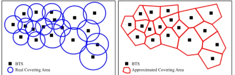
III. INFRASTRUCTURE FORDATAACQUISITION Cell phone networks are built using a set of base transceiver stations (BTS) that are in charge of communicating cell phone devices with the network. The area covered by a BTS is called a cell. A BTS has one or more directional antennas (typically two or three, covering 180 or 120 degrees respectively) that define a sector and all the sectors of the same BTS define the cell. At any given moment in time, a cell phone is covered by one or more antennas. Depending on the network traffic, the phone selects the BTS to connect to. The geographical area covered by a cell depends mainly on the power of the individual antennas. Depending on the population density, the area covered by a cell ranges from less than 1 Km2 in dense urban areas to more than 5 Km2 in rural areas. Each BTS has a latitude and longitude that indicate where is located. For simplicity, we assume that the cell of each BTS is a 2-dimensional non-overlapping region and use Voronoi diagrams to define the covering area of the set of BTSs considered. Figure 1 presents on the left a set of BTSs with the original coverage of each cell, and on the right the simulated coverage obtained using Voronoi. While simple, this approach gives us a good approximation of the coverage area of each BTS. Also, the location of mobile users connected to BTSs are approximated using those Diagrams. In practice, to build the “real” diagram of coverage, one has to consider several factors
Fig. 1. (left) Original coverage areas of BTSs and (right) approximation of coverage areas by Voronoi diagram.
in the mobile network, mainly the power and position of each antenna.
CDR databases are generated when a mobile phone con-nected to the network makes or receives a phone call or uses a service (e.g., SMS, MMS, etc.). In the process, and for invoice purposes, the information regarding the time and the BTS where the user was located when the call was initiated is logged, which gives an indication of the geographical position of a user at a given moment in time. Note that no information about the exact position of a user in a cell is known. Also, it is possible to store for a given call not only the initial BTS, but also the set of BTSs used during the length of the call (BTS hopping option). This allows for a richer representation of the mobility of the users.
In our system we use the set of attributes common to all CDR databases. These include: (1) the phone numberphoneid -O making the call; (2) the phone numberphoneid-D receiving the call; (3) the type of the service (voice: V, SMS: S, MMS: M, etc.); (4) the BTS identifier (BTSid-O) on whichphoneid -O connected to make the call; (5) the BTS identifier (BTSid-D) on whichphoneid-D connected to receive the call; (6) date and time (timestamp) that started the connection betweenphoneid -O andphoneid-D using BTSid-O and BTSid-D, respectively; and (7) the total duration of the call dur between the two parties for BTSid-O and BTSid-D; The BTS identifier will represent the position of the phone number that is a client of the provider keeping the CDR database. If both numbers are part of the provider two BTSs will be present, one indicating the position of the originating number and another one indicating the position of the destination number. When the BTS hopping option is enabled, a new CDR row is created every time either users change their positions. When the hopping is not available, only a single CDR is stored to represent the initial position ofphoneid-O andphoneid-D for the total duration of the call.
TABLE I
ASET OFCDRS REPRESENTING4DIFFERENT CALLS. timestamp dur. phoneid-O phoneid-D BTSid-O BTSid-D type
1123212 3 4324542 4333434 231 121 V 1123215 2 4324542 4333434 232 121 V 1123217 5 4324542 4333434 234 121 V 1123235 2 4324542 5334212 235 231 V 1123237 4 4324542 5334212 231 233 V 1124113 3 4333434 4324541 238 343 V 1124116 4 4333434 4324541 239 231 V 1124116 1 5334212 4333434 451 239 S
Q:= (S [SC])
S:={P1.P2., ..., .Pn},|S|=n Pi:=hopi,Ri[, ti]i opi:=disjoint|meet|overlap|equal|
inside|contains|covers|coveredBy Ri∈ {Σ∪∆∪Γ} ti:= (tf rom:tto)|ts| tr Fig. 2. The STPS Pattern Query Language.
Table I shows an example for 4 different calls where users change their locations during the call. In this example the provider storing the CDR database is all the same and the option of BTS hopping is enabled. The phone number 4324542 makes a phone call at timestamp 1123212 to 4333434 starting in BTS 231. Then the user 4324542 moves from BTS 231 to 232 after 3 minutes of starting the call, generating another input in the database. After 2 miutes, user 4324542 moves to BTS 234 staying there for 5 minutes when the call finishes. The user 4333434 stays connected to the same BTS 121 during the call, which does not necessary means that the user stays on the same place, but connected to the same cell 121 for the whole period of the call. If the BTS hopping was not enabled, the first three entries would have been presented as just one, with just the initial BTS 231 and a total duration of 10 minutes. The second call in the table represents the call made from 4324542 to 5334212, and the third one from 4333434 to 4324541. The eigth entry of the table details an SMS sent from 5334212 to 4333434 when they were connected to BTSs 451 and 239, respectively.
IV. THESTPS PATTERNQUERYLANGUAGE The previous section commented how the spatio-temporal information collected by the CDR databases can have two different formats: the first case just collects the BTSs where the user initiated the call and in the second case the whole trajectory during a call is stored (at a BTS level). In general the first case can be considered a subset of the second one. The STPS language is valid for both cases; i.e. we can query for patterns using records for the same call or different calls. This is only possible because we can “enable” temporal predicates for each spatial predicate and, therefore, restrict that user “movements” are associated to a single call. In the next subsections we describe the syntax of the STPS pattern query language and its components: the spatial predicates, the temporal predicates, and the constraints.
A. STPS Language Syntax
A pattern queryQis defined asQ= (S [SC]), whereS is a sequential pattern andC is an optional set of constraints. A phoneidmatches the pattern queryQif it satisfies bothSand C. A sequential pattern S is expressed as a path expression of an arbitrary numbernof predicatesS ={P1.P2., ..., .Pn}. Figure 4 details formally the syntax of the STPS language.
Each spatio-temporal predicate Pi is defined by a triplet Pi = hopi,Ri[, ti]i, where opi andRi represent a topologi-cal relationship and a geographitopologi-cal area respectively, and in
combination the spatial part of the predicate, andtirepresents the temporal part of the predicate. The operatoropi describes the topological relationship that the spatial region Ri and an instance in the database must satisfy over the (optional) temporal predicateti.
B. Spatial Predicates
The cells, that represent the covering areas of each BTS, are represented using Voronoi diagrams. Such set of Voronoi diagrams is represented byΣin our language. In the following we use capital letters to represent the set of BT S, Σ =
{A, B, C, ...}. In our pattern language, regions (e.g. districts, neighborhoods, areas of interest, etc) can be defined by a set ofBT Sid, i.e. although the ares represented byΣare fixed, on top of that geographical maps with different granularity can be defined. For instance, one can define the downtown area by DOW N T OW N ={D, E, H} andM ALL={G}. The sameBT Sid can be assigned to multiple regions and not all BTS have to be included in each geographical map.
InPi, the areaRi can be one of the four following region specifiers: a particularBT Sid ∈ Σ; an alias A ∈ ∆ defined by a set of one or moreBT Sid; a polygon defined by a set of pairs< longitude, latitude >; or a variableV ∈Γ.
We have used the eight topological relationships: disjoint, meet, overlap, equal, inside, contains, covers and coveredBy, for opi described in [13]. Given an instance of the CDR database CDRj and a region Ri, the operator opi returns a boolean value B ≡ {true, f alse} whether the CDRj and the regionRi satisfy the topological relationshipopi(e.g., an Inside operator will be true if the user associated withphoneid was sometime inside regionRi during timeti). For simplicity in the following we assume that the spatial operator is set to Inside and it is thus omitted from the query examples.
A predefined region (i.e.,Ri∈Σ∪∆) is explicitly specified by the user in the query predicate. In contrary, a variable de-notes an arbitrary region and it is denoted by a lowercase letter preceded by the “@” symbol (e.g. “@x”). A variable region is defined using symbols in Γ, where Γ = {@a,@b,@c, ...}. Unless otherwise specified, a variable takes a single value (instance) fromΣ(e.g.@a=C); however, in general, one can also specify the possible values of a variable as a subset of Σ (e.g., “any city district with museums”). Conceptually, variables work as placeholders for explicit spatial regions and can become instantiated (bound to a specific region) during the query evaluation in a process similar to unification in logical programming.
Moreover, the same variable “@x” can appear in several different predicates of pattern S, referencing to the same region everywhere it occurs. This is useful for specifying complex queries that involve revisiting the same region many times. For example, a query like “@x.B.@x” finds users that started from some region (denoted by variable “@x”), then at some point passed by region B and immediately after they visited the same region they started from.
C. Temporal Predicates
A predicatePi may include an explicit temporal constraint ti in the form of: (a) interval time (tf rom : tto) where tf rom ≤ tto; (b) snapshot time ts; (c) or (d) relative time tr = ti−ti−1 to a previous ti−1 spatio-temporal predicate Pi−1. This implies that the spatial relationship opi between a CDRi and region Ri should be satisfied in the specified timeti (e.g. “passed by areaB between 10am and 11am”). If the temporal constraint is missing, we assume that the spatial relationship can be satisfied any time in the duration of a call. For simplicity we assume that if two predicatesPi, Pj occur within patternS (wherei < j) and have temporal constraints ti, tj, respectively, then these intervals do not overlap and ti occurs beforetj on the time dimension.
D. Pattern Constraints
Spatio-temporal predicates however cannot answer queries with constraints (for example, “best-fit” type of queries – like NN and the related – that find user which best match a specified pattern). This is because topological predicates are binary and thus cannot capture distance based properties of the users. The optional C part of a general query Q is thus used to describe distance-based or other constraints among the variables used in the S part. A simple kind of constraint can involve comparisons among the used variables (e.g.,@x!=@y). More interesting is the distance-based constraint which have the form(AGGR(d1, d2, ...);θ)and is described below. E. STPS Language Examples
The use of variables in describing both the topological pred-icates and the numerical conditions provides a very powerful language to query patterns. To describe a query, the user can use fixed regions for the portions of the users movement where the behavior should satisfy known (strict) requirements, and variables for portions where the exact behavior is not known (but can be described by a sequence of variables and the constraints between them). The ability to use the same variable many times in the query allows for revisiting areas, while the ability to refer to these variables in the distance functions allows for easy description of NN and related queries.
3 COMPEX EXAMPLES HERE EXAMPLES ARE NEEDED in this section, EITHER IN A SUBSECTION OR IN THE TEXT.
V. QUERYEVALUATIONSYSTEM
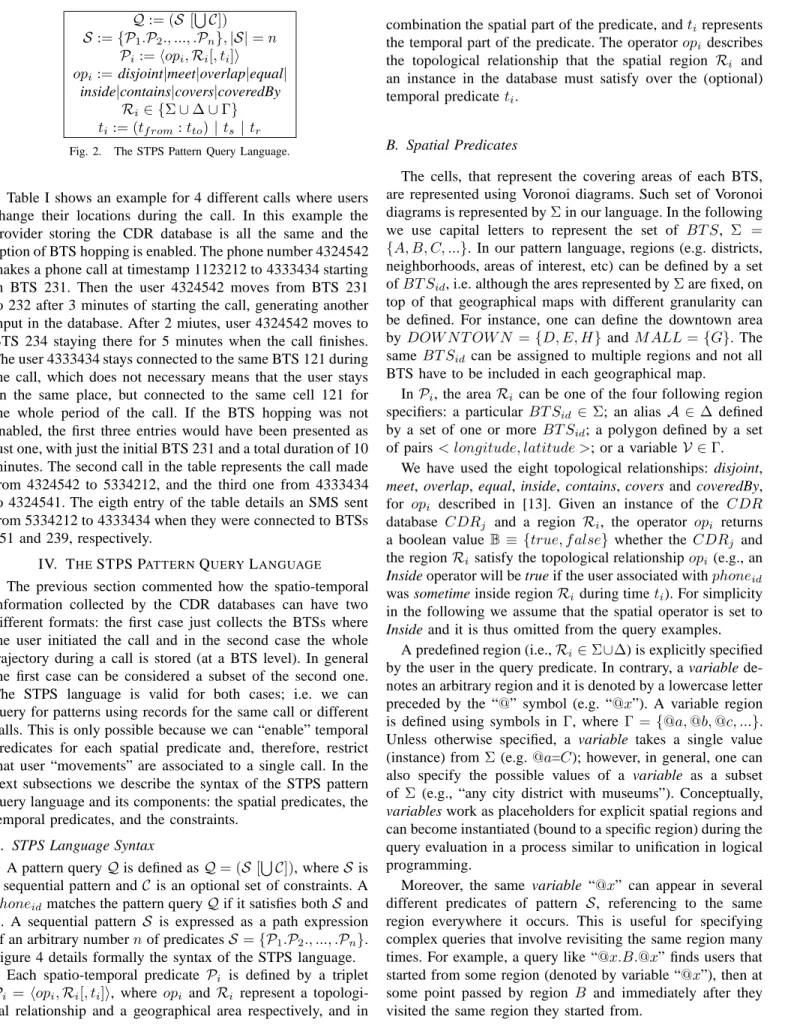
In order to efficiently evaluate pattern queries we use three index structures: one R-tree for the regions; one B+-tree for each BT Sid; and oneinverted-index for each BT Sid. Along with these indexes we also store all CDR in an archive, grouped by phoneid and ordered by timestamp, as shown in Figure 3. The R-tree is used when there is a spatio-temporal predicate inSthat is a polygon type. In this case, the R-tree is evaluated in order to return the set ofBT Sid that satisfies the topological operator that contains the polygon. In case where the result set contains more than one BT Sid, then entries in each BT Sid can be merged to form a unique list with all
entries to be further processed by our algorithm. This is only possible because entries in each list BT Sid has its entries ordered by (phoneid,timestamp) key.
For each BT Sid, two index structures are built: one B+ -tree to organize entries by the temporal attribute times-tamp, and one inverted-index where entries are ordered by (phoneid,timestamp). The B+-tree may be used to prune entries that do not satisfy a temporal predicate. The strategy of using or not the B+-tree will depend on the type of temporal predicate that is being evaluated (more discussion later in this section). The inverted-index of a givenBT Sid stores all call records that were connected to BT Sid in sometime during the call. In the inverted-index each entry inBT Sid is a record that contains a phoneid, the timestamp and duration during which the user was inside regionBT Sid, and a pointer to the CDR record associated to the call in the CDR archive. If a user connects to a given BT Sid multiple times in different timestamps, we store a record for each uses. Records in an inverted-index are ordered first by the phoneid and then by timestamp. For example, in Figure 3 the inverted-index entry for the region D is {4324542,10-01-09 10:23:45,35; 4324542,10-01-09 10:59:12,01; ...}. Note that records from an inverted-index point to the corresponding CDR call in the CDR archive. For example, the record 4324542,10-01-09 10:23:45,35 in the inverted-index14233contains a pointer to the CDR record of 4324542.
For evaluating pattern queries we propose the Index Join Pattern (IJP) algorithm. This algorithm is based on a merge-join operation performed over the inverted-indexes correspond-ing to every fixed predicate in the query patternS.
A. The Index-Join Pattern Algorithm (IJP)
To simplify the presentation we first start with the evaluation of the spatial predicates for a patternS. Later we extend the discussion to cover queries that in addition contain predicate constraints C. Finally we present the incorporation of time constraints inside the pattern queryQ.
1) Spatial Predicate Evaluation: We start with the case where the pattern S does not contain any explicit temporal constraints. In this scenario, the pattern specifies the order by which its predicates (whether fixed or variable) need to be satisfied. Assume S containsn predicates and let Sf denote the set of f fixed predicates, while Sv denotes the set of v variable predicates (n=f+v). The evaluation of S with the IJP Algorithm can be divided in two steps: (i) the algorithm evaluates the set Sf using the inverted-index index to fast prune users that do not qualify for the answer; (ii) then the collection of candidate users is further refined by evaluating the set ofSv.
(i) Fixed predicate evaluation: All f fixed predicates in Sf can be evaluated concurrently using an operation similar to a “merge-join” among their inverted-indexes Li, i∈ 1..f. Records from these f lists are retrieved in sorted order by (phoneid,timestamp) and then joined by their phoneid’s. Records are pruned using thephoneids and timestamp. In each listLi we keep a pointerpi that points to the record currently
Fig. 3. Index framework: (a) BTS R-tree, (b) B+-trees (timestamp), (c) inverted-indexes, and (d) CDR database.
considered for the join. This pointer scans the list starting from the top.
If the same region appears more than once in the patternS, a separate pointer traversing that inverted-index is used for each region appearance in the pattern. For example, to process the patternM.D.Mthe inverted-indexes ofM andDare accessed using one pointer for inverted-indexLD(pD) and two pointers for traversing inverted-index M (pM1 andpM2). If a phoneid
appears in all of thef inverted-indexes involved inS, and their corresponding timestamps in allf inverted-indexes satisfy the ordering of the predicates in S, this phoneid is saved as a possible solution. The pseudo code is shown in Algorithm V-A.2.
During the merge-join, there are cases where records from the inverted-index can be skipped, thus resulting in faster processing. For example, assume that predicate Pi ∈ S (corresponding to the inverted-index Li) is before predicate Pj ∈ S (corresponding to Lj). Further assume that in list Li the current record considered for the join has phone identifier phoner, while in list Lj the current record considered has phone identifier phones. If phones < phoner, processing in list Lj can skip all its records with phoneid < phoner. That is, the pointer pj in list Lj can advance to the first record with phoneid ≥phoner. Essentially, predicate Pi cannot be satisfied by any of the phones in Lj with smaller phoneid than phoner. Since records in a inverted-index are sorted by phoneid,Li does not contain phones with smaller identifiers thanr.
Similarly, when a record from the same phoneid (e.g. phones) is found in two inverted-indexes (e.g. Li,Lj), the algorithm checks whether the corresponding timestamps of the records match the order of predicates in the pattern S. Hence a phoneid that satisfiesS should visit the region ofLi before visiting the region of Lj. If the record of phones in Li has timestamp that falls after the corresponding timestamp of phones in list Lj, this record can be skipped in Li, since it cannot satisfy the query. Since inverted-indexes are
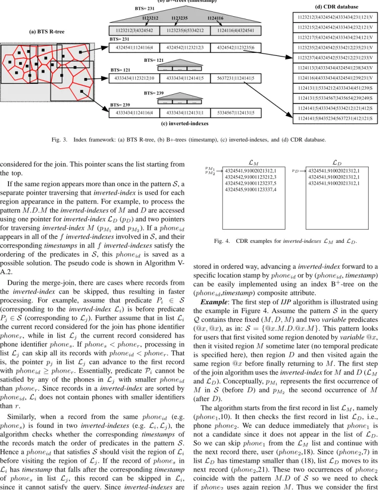
LM pM1 pM2 4324541,91002021312,1 4324542,91001123212,3 4324542,91001123237,5 4324545,91001123337,4 LD pD 4324541,91002021312,1 4324541,91002021312,1 4324541,91002021312,1
Fig. 4. CDR examples for inverted-indexes LM andLD.
stored in ordered way, advancing a inverted-index forward to a specific location stamp byphoneidor by (phoneid, timestamp) can be easily implemented using an index B+-tree on the (phoneid,timestamp) composite attribute.
Example: The first step of IJP algorithm is illustrated using
the example in Figure 4. Assume the pattern S in the query Qcontains three fixed (M, D, M) and two variable predicates (@x,@x), as in:S ={@[email protected]}. This pattern looks for users that first visited some region denoted by variable@x, then it visited regionM sometime later (no temporal predicate is specified here), then region D and then visited again the same region @xbefore finally returning to M. The first step of the join algorithm uses the inverted-index forM andD(LM andLD). Conceptually,pM1 represents the first occurrence of
M in S (before D) and pM2 the second occurrence of M
(afterD).
The algorithm starts from the first record in listLM, namely (phone1,10). It then checks the first record in list LD, i.e., phone phone2. We can deduce immediately that phone1 is not a candidate since it does not appear in the list of LD. So we can skip phone1 from the LM list and continue with the next record there, user (phone2,18). Since (phone2,7) in listLD has timestamp smaller than (18), listLD moves to its next record (phone2,21). These two occurrences of phone2 coincide with the pattern M.D of S so we need to check if phone2 uses again region M. Thus we consider the first
Algorithm 1 IJP: Spatial Predicate Evaluation
Require: QueryS
Ensure: Phones satisfying fixedSf and variableSvpredicates
1: f← |Sf| ⊲number of fixed predicates inS
2: fori←1tof do ⊲for eachSf
3: InitializeLiwith the cell-list ofPi
4: Candidate SetU ← ∅
5: forw←1to|L1|do ⊲analyze each entry inL1
6: p1=w ⊲set the pointer forL1
7: forj←2tof do ⊲examine all other lists
8: ifL1[w].id6∈ Ljthen
9: break ⊲L1[w].iddoes not qualify
10: Letkbe the first entry forL1[w].idinLj
11: whileL1[w].id=Lj[k].idandLj−1[pj−1].t >Lj[k].t do
12: k←k+ 1 ⊲alignLj−1[pj−1].tand Lj[k].t
13: ifL1[w].id6=Lj[k].idthen
14: break ⊲L1[w]does not qualify
15: else pj=k ⊲set the pointer forLj
16: ifL1[w]qualifies then
17: U ←U∪ L1[w].id ⊲L1[w]satisfy allSf
18: if|Sv|= 0then ⊲pattern does not have variable predicate
19: Answer←U
20: else ⊲variable predicate evaluation
21: Answer← ∅
22: fork←0to|U|do
23: Retrievephoneidassociated withU
24: Build segmentsSegiforphoneid
25: Generate variable lists
26: Join variable lists
27: ifphoneid qualifies then
28: Answer←Answer∪phoneid⊲Addphoneid to the answer set
record of listLM usingpM2, namely user (phone1,10). Since
it is not fromphone2 it cannot be an answer so pointerpM2
advances to the next record (phone2,18). Now pointers in all lists point to records ofphone2. However, (phone2,18)inpM2
does not satisfy the pattern since its timestamp should follow the timestamp (21) of phone2 inD. Hence pM2 is advanced
to the next record, which happens to be (phone2,25). Again we have a record from the same user phone2 in all lists and this occurrence of phone2 satisfies the temporal constraints and thus the patternS. As a result, user phone2 is kept as a candidate in U. The processing moves to the next record in pM1, namely (phone2,25). However, this record cannot satisfy
the pattern S so it is skipped. EventuallypM1 will points to
(phone3,10) which causes listpDto move to (phone3,5). User phone3cannot satisfy the temporal constraint, so it is skipped from list LD and the algorithm terminates since one of the lists reached its end.
In cases where a spatial predicate Pi in S is defined by a polygon region, then the above join algorithm has to materialize a sorted inverted index from the set of inverted-indexes satisfying the topological operatoropi over the poly-gon of Pi. However, since records in each set of regions satisfying the spatial predicate Pi are already ordered by (phoneid,timestamp), the sort order can be materialized on the fly (by feeding the algorithm with the record that has the smallest phoneid among the heads of the participating
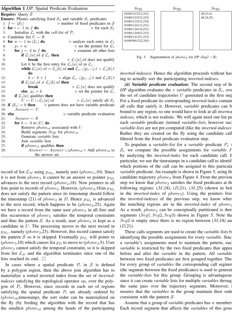
Seg1 (91001123212,231) (91001123215,232) (91001123512,234) (91001124113,231) (91001124116,231) (91001124923,233) (91001141251,232) (91003091232,245) Seg2 Seg3 (H,23,4) (B,24,25)
Fig. 5. Segmentation ofphone2for IJP (Seg2 =∅).
inverted-indexes). Hence the algorithm proceeds without hav-ing to actually sort the participathav-ing inverted-indexes.
(ii) Variable predicate evaluation: The second step of the
IJP algorithm evaluates the v variable predicates inSv, over the set of candidate trajectoriesU generated in the first step. For a fixed predicate its corresponding inverted-index contains all calls that satisfy it. However, variable predicates can be bound to any region, so one would have to look at all inverted-indexes, which is not realistic. We will again need one list per each variable predicate (termed variable-list), however such variable-lists are not pre-computed (like the inverted-indexes). Rather they are created on the fly using the candidate calls filtered from the fixed predicate evaluation step.
To populate a variable-list for a variable predicate Pj ∈ Sv we compute the possible assignments for variable Pj by analyzing the inverted-index for each candidate call. In particular, we use the timestamps in a candidate call to identify which portions of the call can be assigned to this particular variable predicate. An example is shown in Figure 5, using the candidate trajectoryphone2from Figure 4. From the previous step we know thatphone2satisfies the fixed predicates at the following regions: (M,18), (D,21), (M,25) (shown in bold in the inverted-index of phone2). Using the pointers from the inverted-indexes of the previous step, we know where the matching regions are in the inverted-index of phone2. As a result, phone2 can be conceptually partitioned is three segments (Seg1, Seg2, Seg3) shown in Figure 5. Note that Seg2 is empty since there is no region between (M,18) and (D,21).
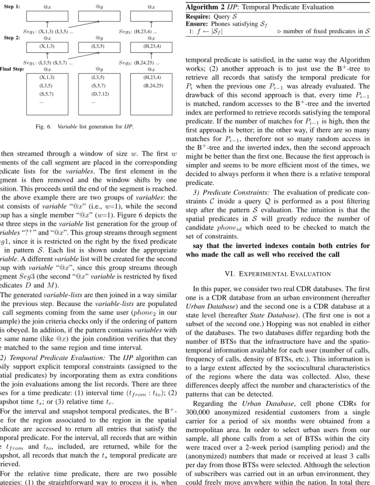
These calls segments are used to create the variable-lists by identifying the possible assignments for every variable. Since a variable’s assignments need to maintain the pattern, each variable is restricted by the two fixed predicates that appear before and after the variable in the pattern. All variables between two fixed predicates are first grouped together. Then for every group of variables the corresponding call segment (the segment between the fixed predicates) is used to generate the variable-lists for this group. Grouping is advantageous, since it can create variable lists for multiple variables through the same pass over the trajectory segments. Moreover, it ensures that the variables in the group maintain their order consistent with the patternS.
Assume that a group of variable predicates haswmembers. Each record segment that affects the variables of this group
Step 1: @x Seg1: (X,1,3) (I,3,5) ... @y @x Seg3: (H,23,4) ... Step 2: @x (X,1,3) Seg1: (I,3,5) (S,5,7) ... @y (I,3,5) @x (H,23,4) Seg3: (B,24,25) ... Final Step: @x (X,1,3) (I,3,5) (S,5,7) ... @y (I,3,5) (S,5,7) (D,7,12) ... @x (H,23,4) (B,24,25)
Fig. 6. Variable list generation for IJP.
is then streamed through a window of size w. The first w elements of the call segment are placed in the corresponding predicate lists for the variables. The first element in the segment is then removed and the window shifts by one position. This proceeds until the end of the segment is reached. In the above example there are two groups of variables: the first consists of variable “@x” (i.e., w=1), while the second group has a single member “@x” (w=1). Figure 6 depicts the first three steps in the variable list generation for the group of variables “?+” and “@x”. This group streams through segment Seg1, since it is restricted on the right by the fixed predicate M in pattern S. Each list is shown under the appropriate variable. A different variable list will be created for the second group with variable “@x”, since this group streams through segmentSeg3(the second “@x” variable is restricted by fixed predicatesD andM).
The generated variable-lists are then joined in a way similar to the previous step. Because the variable-lists are populated by call segments coming from the same user (phone2 in our example) the join criteria checks only if the ordering of pattern S is obeyed. In addition, if the pattern contains variables with the same name (like@x) the join condition verifies that they are matched to the same region and time interval.
2) Temporal Predicate Evaluation: The IJP algorithm can easily support explicit temporal constraints (assigned to the spatial predicates) by incorporating them as extra conditions in the join evaluations among the list records. There are three cases for a time predicate: (1) interval time(tf rom:tto); (2) snapshot time ts; or (3) relative timetr.
For the interval and snapshot temporal predicates, the B+ -tree for the region associated to the region in the spatial predicate are accessed to return all entries that satisfy the temporal predicate. For the interval, all records that are within the tf rom and tto, included, are returned, while for the snapshot, all records that match the ts temporal predicate are retrieved.
For the relative time predicate, there are two possible strategies: (1) the straightforward way to process it is, when the spatial predicate is being evaluated, check whether the
Algorithm 2 IJP: Temporal Predicate Evaluation
Require: QueryS
Ensure: Phones satisfyingSf
1: f← |Sf| ⊲number of fixed predicates inS
temporal predicate is satisfied, in the same way the Algorithm works; (2) another approach is to just use the B+-tree to retrieve all records that satisfy the temporal predicate for Pi when the previous one Pi−1 was already evaluated. The drawback of this second approach is that, every time Pi−1 is matched, random accesses to the B+-tree and the inverted index are performed to retrieve records satisfying the temporal predicate. If the number of matches forPi−1is high, then the first approach is better; in the other way, if there are so many matches for Pi−1, therefore not so many random access in the B+-tree and the inverted index, then the second approach might be better than the first one. Because the first approach is simpler and seems to be more efficient most of the times, we decided to always perform it when there is a relative temporal predicate.
3) Predicate Constraints: The evaluation of predicate con-straints C inside a query Q is performed as a post filtering step after the pattern S evaluation. The intuition is that the spatial predicates in S will greatly reduce the number of candidate phoneid which need to be checked to match the set of constraints.
say that the inverted indexes contain both entries for who made the call as well who received the call
VI. EXPERIMENTALEVALUATION
In this paper, we consider two real CDR databases. The first one is a CDR database from an urban environment (hereafter Urban Database) and the second one is a CDR database at a state level (hereafter State Database). (The first one is not a subset of the second one.) Hopping was not enabled in either of the databases. The two databases differ regarding both the number of BTSs that the infrastructure have and the spatio-temporal information available for each user (number of calls, frequency of calls, density of BTSs, etc.). This information is to a large extent affected by the sociocultural characteristics of the regions where the data was collected. Also, these differences deeply affect the number and characteristics of the patterns that can be detected.
Regarding the Urban Database, cell phone CDRs for 300,000 anonymized residential customers from a single carrier for a period of six months were obtained from a metropolitan area. In order to select urban users from our sample, all phone calls from a set of BTSs within the city were traced over a 2-week period (sampling period) and the (anonymized) numbers that made or received at least 3 calls per day from those BTSs were selected. Although the selection of subscribers was carried out in an urban environment, they could freely move anywhere within the nation. In total there are around 50,000,000 entries in the database considering
voice, SMS and MMS. The BTS database contained the position of 30,000 towers.
As for the State Database, we considered 500,000 users from a state for a period of six months. No selection of users was made, i.e. all users that made or received a phone call from any BTS of that particular state during a six month period were part of the database. In total there were close to 30,000,000 entries in the database. The BTS database contained the position of 20,000 towers.
We randomly sampled 500 phone users from each database to generate sample queries. For each sample phone user we then randomly selected fragments in its history of calls to generate queries with 4, 8, 12 and 16 predicates. Hence, these queries return at least one entry in their respective databases. For each experiment we measured the average query running time and total number of I/O for 500 queries. The query run-ning time reports the average computational cost (as the total wall-clock time, averaged over a number of executions) for 500 queries. To maintain consistency, we set page size equals to 4KBytes for indexes and data structures. All experiments were run on a Dual Intel Xeon E5540 2.53GHz running Linux 2.6.22 with 32 GBytes memory.
For evaluation purposes, we compared the IJP algorithm against a modified implementation of the KMP common subse-quence matching algorithm. We modified the KMP algorithm in a way that it can handle variables, temporal predicates and all topological predicates proposed in our language. This implementation performs a sequential scanning of the CDR database in order to find matches to a particular pattern query. A. IJP vs KMP Comparison
Since the differences in performance between the KMP and the IJP are very large, the plots of the KMP algorithm from all graphs were supressed in order to preserve details. Instead, we describe the results of the KMP here in this section. The total number of I/O measured for the KMP execution is constant in both databases since it performs a sequential scanning of the phone database. For the State database the total number of I/O is 1,788,384, while for the Urban it is 2,022,020. These values correspond to the total number of data disk pages each database has. Comparing these values to the IJP execution, the KMP algorithm performs at least 18 times more I/O than the IJP (for patterns with 2 range predicates with a large window size each for the Urban database). This difference is much greater if only spatial predicates are considered. For example, for patterns with 4 spatial predicates the difference in total number of I/O is 108 times for the State databases, and 260 times for the Urban database.
The query running time of the KMP algorithm on its best performance (patterns with 4 spatial predicates for the Urban database) is on average 853 seconds. For the same kind of queries, the IJP spends on average 0.85s per query, making it 1000 times faster than the KMP algorithm to complete the same task. Even though the cost related to I/O operations is constant when increasing the number of predicates for the KMP algorithm, the running time is not. The total time to
evaluate patterns with larger number of predicates increases substantially. This is due to the fact that more predicates has to be matched to an instance of the phone call.
B. Patterns with Spatial Predicates
The first set of experiments evaluates patterns with different number of spatial predicates (from 4 to 16 patterns). Figure 7 shows the total number of I/O (first row) and query runtime time (second row). For this kind of queries only the inverted indexes associated with the predicates in the pattern are accessed. Increasing the number of spatial predicates increases the number of I/O since more entries in each inverted indexes associated to spatial predicates are retrieved. Consequently, the total time to join those indexes also increases. On the average 306 and 41 phone users match for the State and Urban databases, respectively. 15 20 25 30 35 4 8 12 16 Total I/O (x1000) Number of predicates (a) State Database IJP 6 8 10 12 14 16 18 4 8 12 16 Total I/O (x1000) Number of predicates (b) Urban Database IJP 4 4.5 5 5.5 6 6.5 7 4 8 12 16
AVG Query Runtime (s)
Number of predicates (a) State Database IJP 0.6 0.7 0.8 0.9 1 1.1 4 8 12 16
AVG Query Runtime (s)
Number of predicates (b) Urban Database IJP
Fig. 7. Total I/O and query runtime for spatial predicates
C. Patterns with Variable Predicates
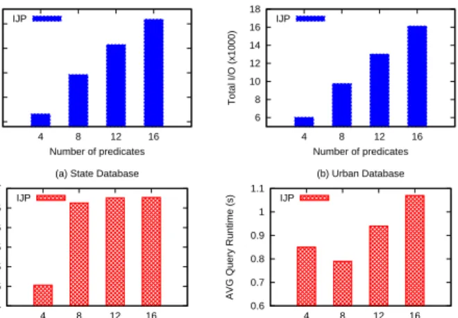
In the second set of experiments we analyze patterns with 1 and 2 variable predicates. In this set of experiments, we randomly selected spatial predicates to be changed to variable predicates. We increase the number of spatial predicates in a similar way as in the previous experiment, maintaining the number of variables to 1 or 2 in the pattern query. For example, patterns with 8 predicates contain 7 spatial and 1 variable predicate for the experiments with 1 variable, and 6 spatial and 2 variable predicates for the experiments with 2 variables. Figure 8 show the performance of the IJP algorithm when varying the number of spatial predicates (from 4 to 16) with 1 variable predicate. The experiments for 2 variables are shown in Figure 9. The total number of I/O for queries with 4 predicates is bigger than for queries with more predicates for some experiments. This is due to the fact that the phone database is accessed once there is a match after the IJP algorithm evaluated the spatial predicates. This behavior is noticed in all the experiments except for the Urban database for patterns with 1 variable.
22 24 26 28 30 32 34 36 4 8 12 16 Total I/O (x1000) Number of predicates (a) State Database IJP 7 8 9 10 11 12 13 14 15 16 4 8 12 16 Total I/O (x1000) Number of predicates (b) Urban Database IJP 5 5.5 6 6.5 7 4 8 12 16
AVG Query Runtime (s)
Number of predicates (a) State Database IJP 0.8 0.85 0.9 0.95 1 1.05 1.1 1.15 1.2 4 8 12 16
AVG Query Runtime (s)
Number of predicates (b) Urban Database IJP
Fig. 8. Total I/O and query runtime for patterns with 1 variable
The difference in the total number of I/O from 1 to 2 variables increases for patterns with 4 predicates. This is due the fact that many more matches occur for 2 spatial predicates (2 variables) than for 3 spatial predicates (1 variable). While in the other cases, this does not happen mainly because more spatial predicates (e.g. 7 spatial predicates) filter out candidates, and therefore, less accesses associated to the phone database are performed. This behavior also happens for the query running time, since less candidates are evaluated.
20 30 40 50 60 70 4 8 12 16 Total I/O (x1000) Number of predicates (a) State Database
IJP 10 15 20 25 4 8 12 16 Total I/O (x1000) Number of predicates (b) Urban Database IJP 4 6 8 10 12 14 16 4 8 12 16
AVG Query Runtime (s)
Number of predicates (a) State Database
IJP 0.5 1 1.5 2 2.5 3 3.5 4 4.5 5 4 8 12 16
AVG Query Runtime (s)
Number of predicates (b) Urban Database
IJP
Fig. 9. Total I/O and query runtime for patterns with 2 variables
D. Patterns with Range Predicates
The same process employed to generate queries with vari-ables were used to generate patterns with range predicates. For this set of experiments we generated a query set with 500 queries with 11 spatial predicates and 1 range predicate, and another query set with 10 spatial predicates and 2 range predicates. To generate range predicates, we randomly selected a spatial predicate to be changed to range predicate. The range predicate correspond to the original spatial predicate location. We then varied the window size in each dimension from 0.004
to 0.02 of its value. For the Urban database, window size of 0.004 selects around 2 BTS, while for 0.02 around 400 BTS are selected. For the State database, 0.02 selects up to 130 BTS due to the fact that the concentration of BTS is not so dense as in the Urban database.
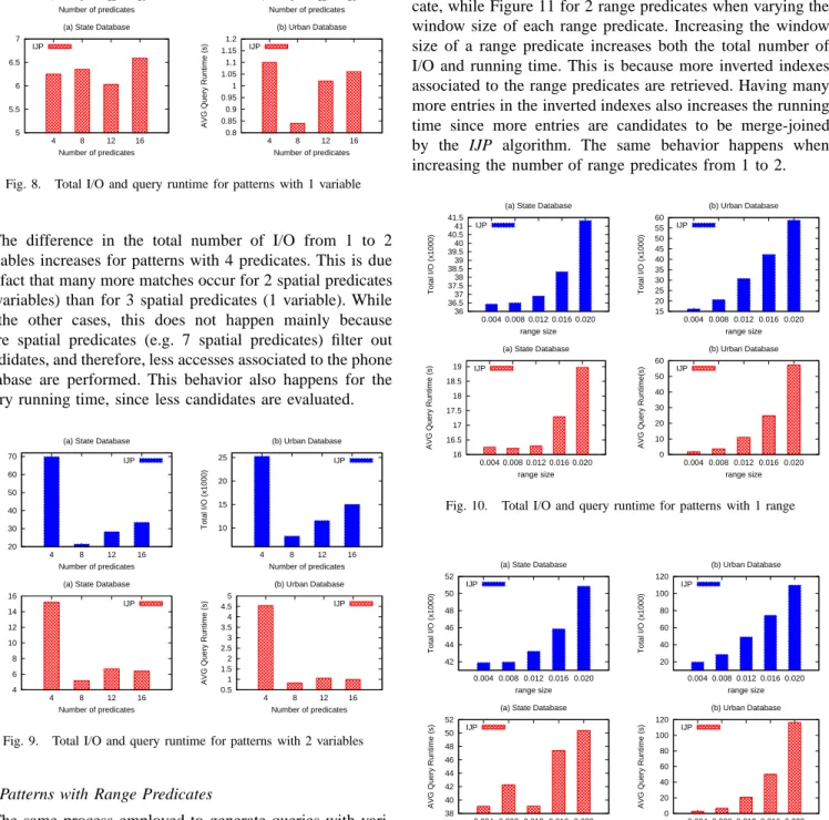
Figure 10 shows the results for queries with 1 range predi-cate, while Figure 11 for 2 range predicates when varying the window size of each range predicate. Increasing the window size of a range predicate increases both the total number of I/O and running time. This is because more inverted indexes associated to the range predicates are retrieved. Having many more entries in the inverted indexes also increases the running time since more entries are candidates to be merge-joined by the IJP algorithm. The same behavior happens when increasing the number of range predicates from 1 to 2.
36 36.5 37 37.5 38 38.5 39 39.5 40 40.5 41 41.5 0.004 0.008 0.012 0.016 0.020 Total I/O (x1000) range size (a) State Database IJP 15 20 25 30 35 40 45 50 55 60 0.004 0.008 0.012 0.016 0.020 Total I/O (x1000) range size (b) Urban Database IJP 16 16.5 17 17.5 18 18.5 19 0.004 0.008 0.012 0.016 0.020
AVG Query Runtime (s)
range size (a) State Database IJP 0 10 20 30 40 50 60 0.004 0.008 0.012 0.016 0.020
AVG Query Runtime(s)
range size (b) Urban Database IJP
Fig. 10. Total I/O and query runtime for patterns with 1 range
42 44 46 48 50 52 0.004 0.008 0.012 0.016 0.020 Total I/O (x1000) range size (a) State Database IJP 20 40 60 80 100 120 0.004 0.008 0.012 0.016 0.020 Total I/O (x1000) range size (b) Urban Database IJP 38 40 42 44 46 48 50 52 0.004 0.008 0.012 0.016 0.020
AVG Query Runtime (s)
range size (a) State Database IJP 0 20 40 60 80 100 120 0.004 0.008 0.012 0.016 0.020
AVG Query Runtime (s)
range size (b) Urban Database IJP
Fig. 11. Total I/O and query runtime for patterns with 2 ranges
E. Patterns with Temporal Predicates
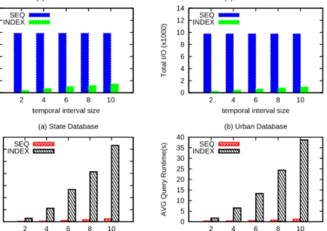
In the last set of experiments we evaluate patterns with temporal predicates (Figure 12). Patterns with temporal predi-cates were generated in a similar fashion as in with spatial
predicates, but here each predicate has both a spatial and an interval temporal predicate. The interval values in each temporal predicate were increased from two days to ten days covering the original timestamp of the call. Therefore, each pattern returns at least one match in the database. The query evaluation is performed in two different ways: the first method (SEQ) validates the temporal predicate while processing each entry in the inverted index for a particular spatial predicate; the second method (INDEX) employs the B+-tree to first evaluate the temporal predicate for each spatial predicate. In INDEX, entries that satisfy the temporal predicate are further sorted by (phoneid, timestamp) to be further processed by the IJP algorithm. 0 5 10 15 20 25 30 35 2 4 6 8 10 Total I/O (x1000)
temporal interval size (a) State Database SEQ INDEX 0 2 4 6 8 10 12 14 2 4 6 8 10 Total I/O (x1000)
temporal interval size (b) Urban Database SEQ INDEX 0 50 100 150 200 250 300 350 2 4 6 8 10
AVG Query Runtime(s)
temporal interval size (a) State Database SEQ INDEX 0 5 10 15 20 25 30 35 40 2 4 6 8 10
AVG Query Runtime(s)
temporal interval size (b) Urban Database SEQ
INDEX
Fig. 12. Total I/O and query runtime for patterns with temporal predicates The total number of I/O for the SEQ method is constant since all pages in the inverted indexes are retrieved. On the other hand, the number of I/O for the INDEX is much smaller than the SEQ approach since only entries that satisfies the temporal predicates are retrieved. Considering the running time for both methods, eventhough the SEQ performs much more I/O operations than the INDEX methods, the way they operate are different: the SEQ method accesses pages in a sequential way while the INDEX method accesses first pages in random order (B+-tree index) and then data pages in sequential order. Furthermore, in INDEX, entries that satisfy the temporal predicate have to be further ordered before being reported to the IJP algorithm. Increasing the interval of a temporal predicate also increases the running time of the INDEX method since the number of entries needed to be sorted increases substantially.
VII. CONCLUSIONS ANDFUTUREWORK
The ability to detect and characterize mobility patterns using CDRs opens the door to a wide range of applications ranging from urban planning to crime or virus spread. Nevertheless, the spatio-temporal query systems proposed so far cannot express the flexibility that such applications require. In this paper we have introduced the Spatio-Temporal Pattern System (STPS) for processing spatio-temporal pattern queries over mobile
phone-call databases. STPS defines a language to express pattern queries which combine fixed and variable spatial predicates with explicit and implicit temporal constraints. We described the STPS index structures and algorithm in order to efficiently process such pattern queries. The experimental evaluation shows that the STPS can answer spatio-temporal patterns very efficiently even for very large mobile phone-call databases. Among the advantages of the STPS is that it can be easily integrated in commercial telecommunication databases and also be implemented in any current commercially available RDBMS. As a next step we are extending the STPS to evaluate continuous pattern queries for streamming data.
REFERENCES
[1] K. Dasgupta and et al., “Social ties and their relevance to churn in mobile telecom networks,” in EDBT, 2008, pp. 668–677.
[2] A. Nanavati and et al., “On the structural properties of massive telecom call graphs: findings and implications,” in ACM CIKM, 2006. [3] M. Seshadri and et al., “Mobile call graphs: beyond power-law and
lognormal distributions,” in ACM SIGKDD, 2008, pp. 596–604. [4] E. Halepovic and C. Williamson, “Characterizing and modeling user
mobility in a cellular data network,” in ACM PE-WASUN, 2005. [5] B. Djordjevic, J. Gudmunsson, A. Pham, and T. Wolle, “Detecting
regular visit patterns,” in ESA, 2008, pp. 244–255.
[6] M. C. Gonzalez, C. A. Hidalgo, and A.-L. Barabasi, “Understanding individual human mobility patterns,” Nature, no. 7196, June 2008. [7] L. Liao, D. J. Patterson, D. Fox, and H. Kautz, “Learning and inferring
transportation routines,” Artif. Intell., vol. 171, no. 5-6, 2007. [8] H. Zang and J. Bolot, “Mining call and mobility data to improve paging
efficiency in cellular networks,” in ACM MobiCom’07, 2007. [9] M. Vieira, P. Bakalov, and V. Tsotras, “Querying trajectories using
flexible patterns,” in UNDER REVIEW, 2009.
[10] R. Sadri and et al., “Expressing and optimizing sequence queries in database systems,” ACM TODS, 2004.
[11] P. Seshadri, M. Livny, and R. Ramakrishnan, “SEQ: A model for sequence databases,” in IEEE ICDE, 1995.
[12] J. Agrawal and et al., “Efficient pattern matching over event streams,”
SIGMOD, pp. 147–159, 2008.
[13] M. Erwig and M. Schneider, “Spatio-temporal predicates,” TKDE, 2002. [14] H. Mokhtar, J. Su, and O. Ibarra, “On moving object queries,” in ACM
PODS, 2002, pp. 188–198.
[15] M. Hadjieleftheriou, G. Kollios, P. Bakalov, and V. Tsotras, “Complex spatio-temporal pattern queries,” in VLDB, 2005, pp. 877–888. [16] C. du Mouza, P. Rigaux, and M. Scholl, “Efficient evaluation of
parameterized pattern queries,” in CIKM, 2005, pp. 728–735. [17] A. Anagnostopoulos and et al., “Global distance-based segmentation of
trajectories,” in ACM KDD, 2006.
[18] Y. Cai and R. Ng, “Indexing spatio-temporal trajectories with Chebyshev polynomials,” in ACM SIGMOD, 2004.
[19] J. Ni and C. Ravishankar, “PA-Tree: A parametric indexing scheme for spatio-temporal trajectories,” in SSTD, 2005.
[20] Y. Yanagisawa, J.-I. Akahani, and T. Satoh, “Shape-based similarity query for trajectory of mobile objects,” in MDM, 2003, pp. 63–77. [21] M. Vlachos, G. Kollios, and D. Gunopulos, “Discovering similar
mul-tidimensional trajectories,” in IEEE ICDE, 2002.
[22] D. Pfoser, C. Jensen, and Y. Theodoridis, “Novel approaches in query processing for moving object trajectories,” in VLDB, 2000.
[23] Y. Tao, D. Papadias, and Q. Shen, “Continuous nearest neighbor search,” in VLDB, 2002, pp. 287–298.
[24] D. Knuth, J. Morris, and V. Pratt, “Fast pattern matching in strings.”
SIAM J. on Computing, 1977.
[25] M. Hadjieleftheriou, G. Kollios, V. Tsotras, and D. Gunopulos, “Index-ing spatiotemporal archives,” VLDB J., pp. 143–164, 2006.
[26] Y. Tao and D. Papadias, “MV3R-Tree: A spatio-temporal access method for timestamp and interval queries,” in VLDB, 2001, pp. 431–440.