GPU-Accelerated SART Reconstruction Using the CUDA
Programming Environment
Benjamin Keck
a,b, Hannes Hofmann
a, Holger Scherl
b, Markus Kowarschik
b, and Joachim
Hornegger
a,ca
Chair of Pattern Recognition, Friedrich-Alexander University Erlangen-Nuremberg, Germany
bSiemens Healthcare, CV, Medical Electronics & Imaging Solutions, Erlangen, Germany
cErlangen Graduate School in Advanced Optical Technologies (SAOT), Friedrich-Alexander
University Erlangen-Nuremberg, Germany
ABSTRACT
The Common Unified Device Architecture (CUDA) introduced in 2007 by NVIDIA is a recent programming model making use of the unified shader design of the most recent graphics processing units (GPUs). The programming interface allows algorithm implementation using standard C language along with a few extensions without any knowledge about graphics programming using OpenGL, DirectX, and shading languages.
We apply this novel technology to the Simultaneous Algebraic Reconstruction Technique (SART), which is an advanced iterative image reconstruction method in cone-beam CT. So far, the computational complexity of this algorithm has prohibited its use in most medical applications. However, since today’s GPUs provide a high level of parallelism and are highly cost-efficient processors, they are predestinated for performing the iterative reconstruction according to medical requirements.
In this paper we present an efficient implementation of the most time-consuming parts of the iterative re-construction algorithm: forward- and back-projection. We also explain the required strategy to parallelize the algorithm for the CUDA 1.1 and CUDA 2.0 architecture. Furthermore, our implementation introduces an ac-celeration technique for the reconstruction compared to a standard SART implementation on the GPU using CUDA. Thus, we present an implementation that can be used in a time-critical clinical environment.
Finally, we compare our results to the current applications on multi-core workstations, with respect to both reconstruction speed and (dis-)advantages. Our implementation exhibits a speed-up of more than 64 compared to a state-of-the-art CPU using hardware-accelerated texture interpolation.
Keywords: CT, CTCB, RECON, CUDA, GPU, SART, OTHER
1. INTRODUCTION
SART1is a well-studied reconstruction method for cone-beam CT scanners. Already ten years ago it was obvious that, in certain scenarios, the Algebraic Reconstruction Techniques (ART) has many advantages over the more popular filtered back-projection2(FBP) approaches. Due to its higher complexity, ART is rarely applied in most of today’s medical CT systems. The typical medical environment requires fast reconstructions in order to save valuable time. Industrial solutions face the performance challenge using dedicated special-purpose reconstruction platforms with digital signal processors (DSPs) and field programmable gate arrays (FPGAs). The most apparent downside of such solutions is the loss of flexibility and their time-consuming implementation, which can lead to long innovation cycles. In contrast, the Common Unified Device Architecture (CUDA) enables a conspicuous simplified development with improved but still limited flexibility. We have already shown that current GPUs offer massively parallel processing capability that can handle the computational complexity of three-dimensional cone-beam reconstruction.3 In 2007 NVIDIA introduced the QuadroFX 5600 architecture (359.3 GFlops∗, 1.4 GHz,
one multiply-add operation per clock cycle per Stream Processor), which uses 128 Stream Processors in parallel.
Further author information: (Send correspondence to Benjamin Keck)
Benjamin Keck: E-mail: [email protected], Telephone: +49 9131 85 28982
Since then, NVIDIA has developed and introduced new CUDA compatible computing architectures with even higher peak performance for solving complex computational problems on the GPU. Recently NVIDIA introduced the QuadroFX 5800 architecture offering 240 Stream Processors for parallel computation. In August 2008 NVIDIA released the second major release of their programming model, CUDA 2.0, enhancing flexibility and extending the hardware feature support.
So far, the iterative reconstruction performance on graphics accelerators has often been evaluated using graphics-based implementation approaches involving OpenGL and shading languages.4, 5 CUDA offers a unified hardware and software solution for parallel computing on CUDA-enabled NVIDIA GPUs supporting the stan-dard C programming language together with high performance computing numerical libraries†. In this paper
we describe our approach for dividing the computational steps and we measure the reconstruction performance using this innovative programming model.
Originating from ART, SART is an iterative method to reconstruct a volumetric object from a sequence of alternating volume projections and corrective back-projections.2 By measuring the difference between the current volume’s forward-projection and the projections acquired by the scanner, a corrective image can be distributed onto the volume grid in the back-projection step. Repeating this correction procedure makes the volume fit to almost all projections or at least minimizes the error in the case of convergence.
Differing from the original ART, where the volume is corrected ray by ray, SART performs a projection-wise correction. This concept becomes the SIRT method when taken one step further to compute all the correction images before they are back-projected onto the volume grid. Ordered Subsets6(OS) approaches are in between SART and SIRT, because they compute a set of corrective images and back-project them before computing the next set of corrective images. Therefore, the projections are partitioned into disjoint sets.
ART-based methods have many advantages over the commonly used FBP and FDK methods7 for 3D cone-beam reconstruction when a full set of projections is not available (e.g., short scan CT or super-short scan CT) or the projections are not distributed uniformly in angle.2 Furthermore, when projections are sparse or missing at certain orientations8, iterative methods can provide superior image quality. If an object is extended beyond the scanning field of view, satisfactory reconstruction results can be produced from incomplete data by applying iterative reconstruction techniques with special constraints.9
Comparing our results to other approaches towards accelerating iterative CT-image reconstruction, Xu et al.10 recently published a similar approach. In their paper the authors report on the efficiency of GPU accelerated iterative reconstruction. Therefore they insist of a general API to use GPUs, neglecting if the API is used for CG or CUDA implementation. Due to the fact of their statement that a ‘write operator can be executed only at the end of a computation’, it is clear that they used OpenGL and shading languages as before.4 With CUDA as the API of choice, this isn’t the case. CUDA allows write operations to the global memory during a kernel execution which is used in our back-projection implementation. In Xu’s approach the volume is represented as a stack of slices (2D arrays) analogous to our CUDA 1.1 approach. Despite from OpenGL and CUDA they have already shown an improved time performance on GPUs for an OS approach compared to the SART method.
In this work, we evaluate the performance of a more advanced reconstruction approach on the current GPU technology. We consider the parallelized implementation and optimization of the SART method for CUDA 1.1 and CUDA 2.0 and introduce a new concept for improving iterative reconstruction speed on GPUs. In the following Section we will briefly review the SART reconstruction theory and describe our CUDA implementation approaches in detail. In Section 3 we will report about the exemplary experiment and the achieved results. Finally, we will conclude our work.
2. METHODS AND IMPLEMENTATION
Algebraic Reconstruction Techniques in principle solve a system of linear equations according to the Kaczmarz method. As introduced SART1 performs a projection-wise correction of the object.
The SART method can be divided into two steps: the corrective image computation (including the forward-projection step, difference computation and scaling) and the back-forward-projection step. In the latter part we use
detector sourceX-ray volume x y z u v
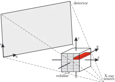
Figure 1. Perspective geometry of the C-arm device (the v-axis and z-axis are not necessarily parallel) together with the parallelization strategy of our back-projection implementation on the GPU using CUDA (thex-z plane is divided in several blocks to specify a grid configuration, and each thread of a corresponding block processes all voxels iny-direction).
our voxel-driven method3 in order to distribute the corrective image onto the volume. For the corrective image computation a forward-projection based on ray casting11 is employed to compute projections of the current volume estimation. The computed projections are then compared to the acquired projections. We adapted our implementation of a CUDA-based ray casting algorithm,12 where we make use of the hardware-accelerated interpolation of textures on graphics cards to compute the trilinearly interpolated samples along each ray.
In theory, the system matrix for the SART defines the forward- and back-projection such that the methods are transposed to each other. In our case, we have an unmatched forward-/back-projector pair for the iterative reconstruction, which has already been investigated.13 The authors demonstrate that an unmatched pair, where the forward-projector is ray-driven while the back-projector is voxel-driven, can effectively remove ring artifacts compared to a matched pair.
Because of deviations due to mechanical inaccuracies of real cone-beam CT systems such as C-arm scanners, the mapping between volume and projection image positions is described by a 3×4 projection matrix Pi for
each X-ray source position i along the trajectory. In a calibration step the projection matrices are calculated only once when the C-arm device is installed. As we use a voxel-based back-projection approach it is required to calculate a matrix vector product for each voxel and projection. However, for neighboring voxels it is sufficient to increment the homogeneous coordinates with the appropriate column of Pi.14 The homogeneous division is
still required for each voxel. It cannot be neglected for a line parallel to thez-axis of the voxel coordinate system since, in general, the projection planes are slightly tilted with respect to this axis (see Figure 1 for an illustration of the perspective geometry of a C-arm device). Due to the fact that the ray direction can be extracted out of the projection matrix, the calibrated geometry is also used in the forward-projection step. We intentionally avoided to use detector re-binning techniques that align the virtual detector to one of the volume axis since this technique decreases the achieved image quality and requires additional computations for the re-binning step.15
One of the important changes between CUDA 1.1 and CUDA 2.0 is the support of 3D textures. We will first review the implementation of the back-projection step, because this is not affected by different CUDA versions. After that we detail the forward-projection step which can exploit the new features of CUDA 2.0.
Back-projection
The back-projection step performs a voxel-based back-projection, which requires the calculation of a matrix-vector product for each voxel in order to determine the corresponding corrective projection value. We invoke our back-projection kernel on the graphics device, where each thread of the kernel computes the back-projection of a certain column and volume slice (see Figure 1).
0 6 12 18 24 0 4 8 12 16 20 24 28 32
Registers per thread
M u lti p ro c e s s o r w a rp o c c u p a n c y
Figure 2. Dependency of the multiprocessor warp occupancy on the register usage. Our CUDA back-projection imple-mentation uses only 10 registers.
8.20 7.65 7.09 7.06 7.14 7.06 6.40 6.60 6.80 7.00 7.20 7.40 7.60 7.80 8.00 8.20 8.40 32x8 64x1 64x2 64x4 128x1 128x2 Grid configuration B a c k -p ro je c ti o n ti m e [s ]
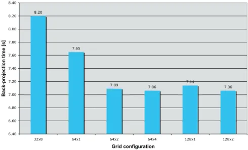
Figure 3. Back-projection execution time example for different grid configurations.
This allows to save six multiply-add operations by incrementing the homogeneous coordinates with the appropriate column ofPifor neighboring voxels iny-direction. This approach also reduces the register usage (see
Figure 2). In this regard, a rectification-based approach has theoretically the potential to further improve the reconstruction speed.15 During our experiments we, however, observed that this is not true for the used graphics hardware. The rectification-based method approach even degrades the reconstruction speed when compared to the approach described above.
An efficient grid configuration for the projection step was chosen experimentally for an arbitrary back-projection configuration (see Figure 3). A more detailed description can be found in Scherl et al.3
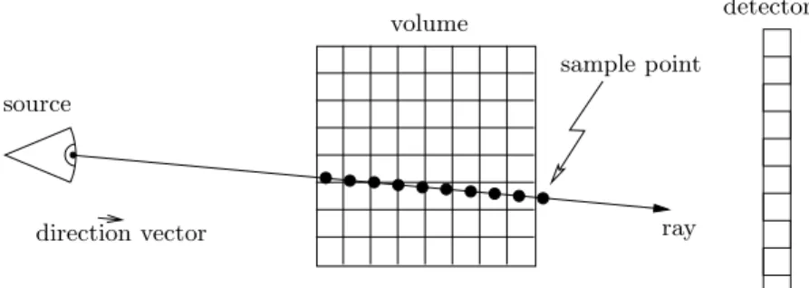
source detector volume ray direction vector sample point
Figure 4. Ray casting principle with an equidistant sample step size.
Corrective image computation
As introduced SART performs a projection-wise correction of the current estimation of the volume. Therefore, the corrective image has to be computed from the difference between the original projection and the appropriate simulated X-ray image of the current reconstruction estimate. All values in the corrective image are finally multiplied by the relaxation factor1before the back-projection step. The implementation principles for CUDA 1.1 and CUDA 2.0 are illustrated in Figures 6 and 7.
A realistic simulation of the X-ray imaging process can be achieved by a ray cast based forward-projection. Research on this grid-interpolated scheme, where the interpolation is performed using a trilinear filter and the integration according to the trapezoidal rule, showed that the root mean square (RMS) error is comparable to other popular interpolation and integration methods used in computed tomography.16 This scheme is our first choice, because it can be ideally mapped to the GPU hardware including hardware-accelerated texture access.
Algorithm 1Forward-projection with a ray casting algorithm
for allprojectionsdo
compute source position out of projection matrix compute inverted projection matrix
for allrays inside the projectiondo
compute ray direction depending on the image plane normalize direction vector
//RAY CASTING
compute entrance and exit point of the ray to the volume
if ray hits the volume then
set sample point to the entrance point initialize the pixel value
while sample point is inside the volumedo
add up the computed sample value at current position to the pixel value compute new sample point for given step size
end while else
set pixel value to zero
end if
normalize pixel value to world coordinate system units
end for end for
The volumetric ray casting principle for the forward-projection step is illustrated in Figure 4 and the algorithm is shown in Algorithm 1. To determine the attenuation value of a certain pixel on the detector plane, a ray is drawn pointing from the X-ray source towards the detector pixel position. Afterwards voxel intensity values inside the volume are sampled equidistantly along the ray. These sampling values add up to the respective
attenuation value in the simulated projection. Similar to the back-projection step we use projection matrices, instead of assuming an ideal geometry, to compute the resulting perspective projection.
To parallelize the forward-projection step, each thread of the kernel computes one corrective pixel of a projection. Analogous to the back-projection step we chose the grid configuration experimental due to our results.12 In the implemented kernel we compute the direction vector for a specific ray, which is the first step in the inner for loop in Algorithm 1. Therefore we take the source position vector and the 3D coordinate of the pixel position, compute the difference vector, and normalize it. The source position for all rays of a projection is obtained from the homogeneous projection matrix which is designed to project a 3D point to the image plane. Depending on the output format of the projection (2D image- vs. 3D world-coordinates), this matrix has three or four rows. In the latter case, the vector can be found in the fourth column of the inverted matrix (first three components). In the case of a 3×4 matrix it is possible to drop the fourth column, invert the 3×3 matrix and
multiply the inverse with the previously dropped fourth column to get the source position. This holds, because in case of a perspective projection with projection matrices, this fourth column represents the shift of the optical center to the origin of the coordinate system. Galigekere et al.17 have shown already how to reproject using projection matrices. − ∗ 2D texture volume projections S1 S2 S3 S4 FP BP update . . . relaxation factor
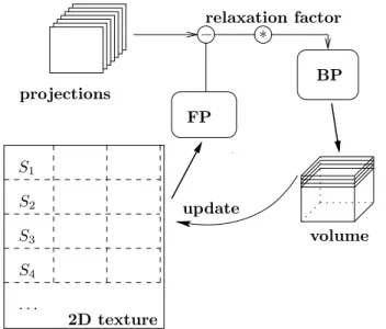
Figure 5. GPU implementation principle: Volume represented in a 2D texture by slices Sj is forward-projected (FP).
After computing the corrective image and scaling with the relaxation factor, the back-projection (BP) distributes the result onto the volume. After performing an update the 2D texture representation of the volume is equal to the volume.
In the kernel code, the inverse of the projection matrix is used to get the ray direction out of the pixel position in the projection image. The entrance and exit positions of the specific ray into the volume are calculated and stored as entrance and exit distances with respect to the source position. Between those points the volume is then sampled equidistantly. To get one sampling position, we take the entry vector and add the direction vector multiplied with the step size times a counter variable. The following sampling step itself proves to be crucial for the algorithm’s efficiency. In order to get satisfying results, a sub-voxel sampling is required, which introduces a trilinear interpolation.
The global memory offers write access and thus has a higher latency. In contrast read-only texture memory has conspicuous low latency due to caching mechanisms and further offers hardware-accelerated interpolation. In CUDA 1.1 the computation of each sample point intensity is a critical issue since support for 3D textures is not provided. In consequence, a workaround had to be applied that used just the bilinear interpolation capability of the GPU. The kernel computes a linear interpolation between stacked 2D texture slices (Sj) (see Figure 6).
Therefore, two values are fetched from proximate stack slices with hardware-accelerated bilinear interpolation and afterwards linearly interpolated in software. These sampling steps are substituted by only one hardware-accelerated 3D texture fetch in CUDA 2.0. Since texture memory is read-only, the back-projection updates the
original volume data kept in global memory. The volume-representing texture has to be synchronized with the updated estimate (Figure 6). Such a synchronization is referred to as a texture update.
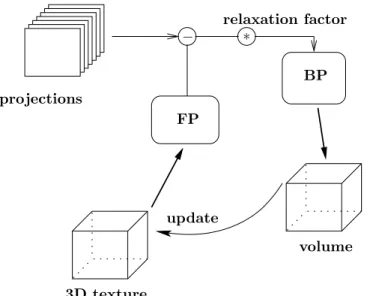
− ∗ 3D texture volume projections FP BP update relaxation factor
Figure 6. GPU implementation principle: Volume represented in a 3D texture is forward-projected (FP). After computing the corrective image and scaling with the relaxation factor, the back-projection (BP) distributes the result onto the volume. After performing an update the 3D texture representation of the volume is equal to the volume.
The difference in volume representation for the corrective image computation leads to two major principles of SART implementation using CUDA shown in Figure 6 for CUDA 1.1 and Figure 7 using CUDA 2.0. After all corrective images have been computed and back-projected for all iterations the reconstruction finishes by transferring the volume to the host system memory.
3. EXPERIMENTS AND RESULTS
In order to evaluate the performance of the GPU vs. the CPU we did the following experiment. On the CPU side we used an existing multi-core based reconstruction framework, while using NVIDIA’s QuadroFX 5600 on the GPU side. Our test data consists of simulated phantom projections, generated with DRASIM.18 We used 228 projections representing a short-scan from a C-arm CT system to perform iterative reconstruction with a projection size of 256×128 pixels. The reconstruction yields a 512×512×350 volume. In order to achieve a
sub-voxel sampling in the forward-projection step we used a step-size of 0.3 of the uniform voxel-size. Since the majority of time in reconstruction is spent on copying the volume data for the reconstructed image from the global memory to a texture memory in order to use the hardware-accelerated interpolation, we can significantly reduce this time by performing an ordered subsets method.
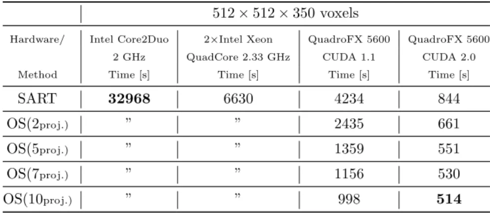
Table 1 shows the achieved performance for the CPU-based SART reconstruction as well as for our optimized GPU implementations using CUDA 1.1 and CUDA 2.0. The former does not need additional memory for the forward-projection step because there is no texture update, and therefore reconstruction times for the SART and OS are identical.
In principle, graphics cards have a very high internal memory transfer rate (≈62 GB/s on the QuadroFX 5600).
Since texture memory is not stored linearly, it has to be reorganized for texture representation, which is the rate-limiting factor using CUDA 1.1. We measured 476 seconds to transfer a 5123 volume 414 times to the texture stack representation. This is approximately 1.15 seconds for a single texture update. Using 3D textures in CUDA 2.0 this can be improved by a factor of 10 such that a texture update can be performed in approximately 0.11 seconds.
512×512×350 voxels
Hardware/ Intel Core2Duo 2×Intel Xeon QuadroFX 5600 QuadroFX 5600 2 GHz QuadCore 2.33 GHz CUDA 1.1 CUDA 2.0 Method Time [s] Time [s] Time [s] Time [s]
SART 32968 6630 4234 844
OS(2proj.) ” ” 2435 661
OS(5proj.) ” ” 1359 551
OS(7proj.) ” ” 1156 530
OS(10proj.) ” ” 998 514
Table 1. Comparison of iterative reconstruction times in seconds (for 20 iterations each).
A SART implementation in CUDA 1.1 wastes approximately 1 second per update to transfer the back-projected volume to a texture memory representation used for the projection. If the number of forward-and back-projections between two texture updates is increased slightly, the reconstruction speed will be faster while the convergence rate remains almost at the same level, but is not as fast as a standard SART (analogous to the relation between ART and SART). This trade-off between convergence and speedup is one of our main results. The convergence was recently examined by Xu et al.10
We compared reconstruction times on three different systems. First, an off-the-shelf PC equipped with an Intel Core2Duo processor running at 2 GHz, second, a workstation with two Intel Xeon QuadCore processors at 2.33 GHz and a NVIDIA QuadroFX 5600 with CUDA 1.1 and 2.0. The SART implementation using CUDA 1.1 is the slowest implementation on the GPU. Yet it is more than 7.5 times faster than the PC and 50 percent faster than the workstation. Employing the ordered subsets optimization yields another speedup of over 4 times. SART with 3D texture interpolation (CUDA 2.0) is even a bit faster, and using OS again results in a total speedup of 64 and 12 compared to the PC (2 cores) and the workstation (8 cores) respectively.
4. CONCLUSION
In conclusion, we have optimized the reconstruction speed and the convergence behavior in our algorithm design. We have shown the advantage of using the texture memory of current graphics cards to perform the most time-consuming parts of an iterative reconstruction technique effectively on the GPU using CUDA 1.1 and recently released CUDA 2.0. Apparently, in CUDA 1.1 the time consuming texture updates dominate the overall reconstruction time. This is dramatically relieved in the CUDA 2.0 implementation. Therefore, the impact of OS with CUDA 2.0 is much lower than with CUDA 1.1.
Furthermore, we have demonstrated the drawback of representing the volume data as a texture in that, it is the time-expensive update process, necessary in iterative reconstruction. Alternatively, the OS method reduces this effect because it requires fewer updates. For a small increase of forward-/back-projections between two update steps, the reconstruction speed is accelerated significantly, while the convergence rate is not decreased significantly. Due to a reconstruction time of less than 9 minutes, our implementation is already applicable for specific usage in the clinical environment.
5. OUTLOOK
Our research also demonstrates that there exists a lack of comparibility for fast 3D reconstruction implementa-tions, despite the plurality of publications. For future research, we want to improve this by providing an open platform –RabbitCT (www.rabbitCT.com)– for worldwide comparison in back-projection performance on differ-ent architectures using a specific high resolution angiographic dataset of a rabbit. This includes a sophisticated interface for rankings, a prototype implementation in C++ and image quality measures.
Acknowledgements
This work is being supported by Siemens Healthcare, CV, Medical Electronics & Imaging Solutions and the In-ternational Max Planck Research School for Optics and Imaging (IMPRS-OI), Erlangen, Germany, the Erlangen Graduate School in Advanced Optical Technologies (SAOT). We wish to give special thanks to Dr. Holger Kunze who supported us with his software framework for iterative reconstruction using multi-core CPUs.
REFERENCES
[1] Andersen, A. and Kak, A., “Simultaneous Algebraic Reconstruction Technique (SART): A superior imple-mentation of the ART algorithm,”Ultrasonic Imaging6, 81–94 (January 1984).
[2] Mueller, K. and Yagel, R., “Rapid 3D cone-beam reconstruction with the Algebraic Reconstruction Tech-nique (ART) by utilizing texture mapping graphics hardware,”Nuclear Science Symposium, 1998. Confer-ence Record. 1998 IEEE3, 1552–1559 (1998).
[3] Scherl, H., Keck, B., Kowarschik, M., and Hornegger, J., “Fast GPU-Based CT Reconstruction using the Common Unified Device Architecture (CUDA),” in [Nuclear Science Symposium, Medical Imaging Confer-ence 2007], Frey, E. C., ed., 4464–4466 (2007).
[4] Mueller, K., Xu, F., and Neophytou, N., “Why do Commodity Graphics Hardware Boards (GPUs) work so well for acceleration of Computed Tomography?,” in [SPIE Electronic Imaging Conference], (2007). (Keynote, Computational Imaging V).
[5] Churchill, M., “Hardware-accelerated cone-beam reconstruction on a mobile C-arm,” in [Proceedings of SPIE], Hsieh, J. and Flynn, M., eds.,6510, 65105S (2007).
[6] Hudson H.M., L. R., “Accelerated image reconstruction using Ordered Subsets of Projection Data,”IEEE Transactions on Medical Imaging13(4), 601–609 (1994).
[7] Feldkamp, L., Davis, L., and Kress, J., “Practical Cone-Beam Algorithm,” Journal of the Optical Society of AmericaA1(6), 612–619 (1984).
[8] Kak, A. and Slaney, M., [Principles of Computerized Tomographic Imaging], SIAM (2001).
[9] Kunze, H., H¨arer, W., and Stierstorfer, K., “Iterative extended field of view reconstruction,” in [Medical Imaging 2007: Physics of Medical Imaging. Edited by Hsieh, Jiang; Flynn, Michael J.. Proceedings of SPIE, Volume 6510, pp. 65105X (2007).], Presented at the Society of Photo-Optical Instrumentation Engineers (SPIE) Conference6510(Mar. 2007).
[10] Xu, F., Mueller, K., Jones, M., Keszthelyi, B., Sedat, J., and Agard, D., “On the Efficiency of Itera-tive Ordered Subset Reconstruction Algorithms for Accelerations on GPUs,” (2008). Workshop on High-Performance Medical Image Computing and Computer Aided Intervention (HP-MICCAI 2008).
[11] Rezk-Salama, C., Engel, K., Hadwiger, M., Kniss, J. M., and Weiskopf, D., [Real-time volume graphics], AK Peters (2006).
[12] Weinlich, A., Keck, B., Scherl, H., Korwarschik, M., and Hornegger, J., “Comparison of High-Speed Ray Casting on GPU using CUDA and OpenGL,” in [High-performance and Hardware-aware Computing (HipHaC 2008)], Buchty, R. and Weiss, J.-P., eds., 25–30 (2008).
[13] Zeng, G. and Gullberg, G., “Unmatched projector/backprojector pairs in an iterative reconstruction algo-rithm,”IEEE Transactions on Medical Imaging19, 548–555 (May 2000).
[14] Wiesent, K., Barth, K., Navab, N., Durlak, P., Brunner, T., Schuetz, O., and Seissler, W., “Enhanced 3-D-reconstruction algorithm for C-arm systems suitable for interventional procedures,”IEEE Transactions on Medical Imaging19(5), 391–403 (2000).
[15] Riddell, C. and Trousset, Y., “Rectification for Cone-Beam Projection and Backprojection,”IEEE Trans-actions on Medical Imaging25(7), 950–962 (2006).
[16] Xu, F. and Mueller, K., “A comparative study of popular interpolation and integration methods for use in computed tomography,”Biomedical Imaging: Nano to Macro, 2006. 3rd IEEE International Symposium on, 1252–1255 (April 2006).
[17] R. Galigekere, K. Wiesent, D. H., “Cone-Beam Reprojection Using Projection-Matrices,”IEEE Transactions on Medical Imaging22(10), 1202–1213 (2003).