Efficient Estimation of Linear Asset Pricing Models with Moving-Average Errors

NBER TECHNICAL WORKING PAPER SERIES

EFFICIENT ESTIMATION OF LINEAR ASSET PRICING MODELS WITH MOVING-AVERAGE ERRORS

Lars Peter Hansen Kenneth J. Singleton

Technical Working Paper No. 86

NATIONAL BUREAU OF ECONOMIC RESEARCH 1050 Msssachusetts Avenue

Cambridge, MA 02138 March 1990

Pe are grateful to the National Science Foundstion for financial support and to Kobi Boudoukh, Charles Evans, John Heaton, Robin Luinsdaine, Masao Ogaki, Karl Snow and Chi Wa 'Lien for research assistance. John Cochrsne and John Heaton provided helpful comments. The second author is also grateful for support from the Center for Research in Security Prices at The University of Chicago. Portions of this paper were written while the first author was a visiting scholar at the Graduate School of Business at Stanford University. This paper is part of NBER's research program in Financial Markets and Monetary Economics. Any opinions expressed are those of the authors and not those of the National Bureau of Economic Research.

NBER Technical Working Paper #86 March 1990

EFFICIENT ESTIMATION OF LINEAR ASSET PRICING MODELS WITH MOVING-AVERAGE ERRORS

ABSTRACT

This paper explores in depth the nature of the conditional moment restrictions implied by log-linear intertemporal capital asset pricing models (ICAPMs) and shows that the generalized instrumental variables (GMM) estimators of these models (as typically implemented in practice) are inefficient. The moment conditions in the presence of temporally aggregated consumption are derived for two log-linear ICAPMs.

The

first is a continuous time model in which agents maximize expected utility. In the context of this model, we show that there are important asymmetries between the implied moment conditions for infinitely and finitely-lived securities. The second model assumes that agents maximize non-expected utility, and leads to a very similar econometric relation for the return on the wealth portfolio. Then we describe the efficiency bound (greatest lower bound for the asymptotic variances) of the CNN estimators of the preference parameters in these models. In addition, we calculate the efficient CNN estimators that attain this bound. Finally, we assess the gains in precision from using this

optimal CNN estimator relative to the commonly used inefficient CMN

estimators.

Lars Peter Hansen Kenneth J. Singleton Department of Economics Graduate School of Business University of Chicago Stanford University

Chicago, IL 60637 Stanford, CA 94305

1. INTRODUCTION

The testable implications of intertemporal asset pricing theories

(ICAPMs) frequently take the form of conditional moment restrictions on

linear econometric models with moving-average disturbances. Moving-average errors may arise, for example, when multi-period returns are examined [e.g., Hansen and Hodrick (1980,1983), Dunn and Singleton (1986), Faina and French (1988)] or in the presence of time-averaged data [e.g., Barro (1981), Grossman, Melino and Shiller (1987), Hall (1988)1. The combination of moving average disturbances and limited information about distributions1 has led

naturally to estimation of the unknown parameters in these models using the generalized method of moments (GMM). The parameters of multi-period forecast equations are frequently estimated by least squares [Hansen and Hodrick (1980) and Fama and French (1988)], while instrumental variables procedures have been used in estimating simultaneous equations derived from ICAPM5

[Harvey (1988) and Hall (1988)]. For pedagogical purposes it is convenient to view both least squares and instrumental variables estimators as GMM estimators.

rn this paper we explore in depth the nature of the conditional moment restrictions implied by log-linear ICAPM5 and show that GMM estimators of

these models (as typically calculated in practice) are inefficient. The moment restrictions implied by two log-linear ICAPM5 in the presence of temporally aggregated consumption are derived in section 2. The first model

is a continuous time ICAPM which includes the models proposed by Grossman, Melino, and Shiller (1988) and Hall (1988) as special cases. In the context of this model, we show that there are important asymmetries between the moment conditions implied by expected utility models for infinitely and finitely-lived securities. For returns on infinitely-lived securities,

temporal aggregation induces autocorrelations in the disturbances that are known

a

priori, while for some finite-lived securities, the induced autocorrelations are not known

a

priori. Hence, Working's (1960) autocorrelation restriction for temporally aggregated Brownian motions need not apply to log-linear models of returns on short and intermediate term bonds. Whence, imposition of this restriction may lead to inconsistent estimators of standard errors and, in some cases, the preference parameters as well.

The second model studied is a special case of the ICAPM with

non-expected utility proposed by Epstein and Zin (1989a,b) for the return on the wealth portfolio. Though the economic underpinnings of this model and the expected utility ICAPM are different, they are shown to imply strikingly similar econometric equations for this return. Consistent with Hall's (1988) analysis, the parameter on consumption growth in the non-expected utility

model is the intertemporal elasticity of substitution and not the coefficient of relative risk aversion. However, these observations apply only to our expression for the return on the wealth portfolio and, in particular, do not provide a reinterpretation of log-linear models of bond returns.

There is a large (infinite-dimensional) class of GMM estimators for the preference parameters of these log-linear ICAPMs. Drawing upon the analyses in Hansen (1985) and Hansen and singleton (1989), fl

Section

3 we describe the efficiency bound (a greatest lower bound for the asymptotic variances) for this class of estimators, and present a GMM estimator that attains this bound. The GMM estimators typically implemented in practice for linear asset pricing models do not attain this bound because they exploit only a subset of

the implied conditional moment restrictions.

illustrated in the context of least squares estimation in the presence of

moving-average errors. Ever since Fama's (1965) pioneering study of the martingale representation of stock prices, substantial attention has been

given to multi-period optimal linear forecasting equations of the form:

(1.1) 3't+m — +

+

+ &y

+

e,

where the first element of vector is a return, excess return, or difference between a forward and future spot price over m periods.2 The 8.'s in (1.1) are square matrices that are either unrestricted or may depend on some lower-dimensional parameter vector fi. The disturbance term e+ is an

expectational error satisfying E(et+mIIt) — 0, where is generated by current and all past values of Under these assumptions, (er) follows an MA(m-l) process.

Consistent estimators of the Sj'5 (and in the case of a priori restrictions) are commonly obtained using least squares methods that exploit the moment conditions:

(1.2)

E(e+Yj')

—

0,

for j—0,1 p.

When (eu) is serially correlated, least squares is in general not the most

efficient estimation method in the presence of the conditional mean

restriction E(et+mIIt) —

0.

This is because the additional moment conditions

(1.3)

E(e.fYj')

—

0,

j

> p.

The log-linear ICAPMs described in section 2 imply an analogous, infinite collection of moments conditions that can be used in estimating the preference parameters. In section 4 we calculate efficient GM/I estimators that exploit all of the moment restrictions, and assess the gains in precision relative to the commonly used inefficient GM/I estimators. Our calculations exploit the characterization of efficient GM/I escimacors and algorithms for calculating these estimators presented in Hansen (1985) and Hansen and Singleton (1989).

2. LOG-LINEAR, INTUTEMPORAL ASSET PRICING MODELS

In

this section we investigate the conditional moment restrictions implied by two

log-linear,

continuous time ICAPMs linking consumption and asset returns. In the first of these models, consumers have state-separable preferences. This model includes the models studied by Grossman, Melino, and Shiller (1987) and Hall (1988) as special cases. The consumers in second model have preferences that are not state-separable as proposed recently by Epstein and Zin (1989a,b), Kocherlakota (1989) and Weil (1989). The models we consider depart from the assumptions of the log-linear model examined in Hansen and Singleton (1983) by replacing the assumption that the agents' decision interval coincides with the sampling interval of the data (e.g., one

month) with the assumption that agents adjust their consumption and

portfolios more frequently. Although the specifications of preferences in these models are different, they imply similar log-linear asset pricing relations. Therefore, a comparison of the implied relations is instructive for interpreting the conditional moment restrictions implied by log-linear ICAPMs. The implications of this discussion for the relative efficiency of alternative GM)! estimators are pursued in Section 3.

2.A A Continuous Time ICAIM with State-Separable Preferences

Following Grossman, Melino, and Shiller (1987) and Hall (1988), consider a representative consumer who chooses a consumption process (C(t) : tO) to maximize:

(2.1) exp(-6t)U[C(t)]dt

utility function U is:

(2.2) U(C) — - 1 ,

y

< 0

7+1

The marginal utility process associated with (2.2) is

(2.3) MU(t) —

exp(-fc(t)]

where c(t) —

log[C(t)].

Infinitely-Lived Securities

As in Grossman, Melino and Shiller (1987), we posit a price process for an infinitely-lived asset and deduce restrictions relating the equilibrium behavior of this price process to consumption. The price process presumes

that all dividends are reinvested in the security and that the entire return is measured by the capital gain or price appreciation. Let Q(t) denote the price in terms of consumption of this security, and q(t) —

log[Q(t)]

An implication of a large class of intertemporal asset pricing models is that in equilibrium the process (etMU(t)Q(t) : t?0) is a martingale adapted to the increasing sequence of agents' information sets (1(t)

(2.4) E(eS(t+MU(t+r)Q(t+r)$I(t)] —

etMU(t)Q(t)

for all rO. Since our focus is on estimation of linear models, we impose the additional assumption that

(2.6) d[MU(t)Q(t)] —

6MtJ(t)Q(t)dt

+ MU(t)Q(t)[a.dW(t)]

where (W(t) : tO) is a vector of uncorrelated Brownian motions adapted to (1(t) : taO) and the vector of real numbers c is constant over time. Since W(t) may be a vector, (2.6) allows multiple sources of uncertainty to affect Q(t) and C(t). Without loss of generality, we assume E[W(t)W(t)'] —

tI.

Relation (2.6) is consistent with the assumptions about the distributions of C(t) and Q(t) in Grossman, Melino and Shiller (1987) and Hall (1988). Using Ito's Lemma, the corresponding expression for logarithms is

(2.7) d(log(MU(t)Q(t)]) —

-)dt

+ a.dW(t)

That

is, ([7c(t) + q(t)] : tal) is a Brownian motion with drift 6-(c.c/2). From (2.7) it follows that

(2.8) [ic(t+l) + q(t+l)) —

[yc(t)

+ q(t)] + -

j) +

_{o.W(t+l) -}

o.W(t)

Suppose only discrete time data are available for studying (2.8). Typically, studies of (2.8) (e.g., Hansen and Singleton (1983), Ferson (1983)] have assumed that the decision interval of agents coincided with the sampling interval of consumption. However, several authors, including Grossman, Melino and Shiller (1987), and Hall (1988), have suggested that

discrete time consumption data be viewed instead as a geometric average over time of the instantaneous consumption flows. Under this interpretation, a version of (2.8) expressed in terms of measured variables is obtained by

averaging (2.8) backward over one unit of time:

(2.9)

[Ca(+l) -

Ca(fl

+ [qa(t+l) -

qa(t)]

-[6

-

Ua(÷l)

where

(2.10) u5(t+l) —

J

a.W(t+1-r)dr

-

Jc.W(t.r)dr

and Ca()

etc. Notice that [qa(t+l) -

qa(t)]

is a geometric average over time of real returns. Equation (2.9) is the econometric model that will be investigated empirically.

There are two implications of this model that can be tested using time series data. First,

(2.11) E[ua(t+2)II(t)] -

0

Second, as shown in Working (1960) the first-order autocorrelation of the

temporally aggregated first difference of a Brownian motion equals .25:

(2.12) E[.25 ua(t+2)2 -

u(t+2)u(t+].)II(t)]

—

0

Both of these conditional moment restrictions can be tested using discrete time data

without

having to parameterize the continuous time law of motion for ([c(t),q(t)1 : t0). To see this in the case of (2.11), let x(t) be any vector of variables observed by agents and the econometrician at date t,

let

and Pq denote the vector of coefficients in the regressions of [Ca(÷2)

-and (q&(t+2)

q(4)] onto x(t). respectively, and let and denote the coefficients on the constants in these two

regressions.

Then (2.11) implies that —

Pq

which identifies '

as

long as p 0 0, and leads

to overidentifying restrictions. Once

is

identified, he discount rate 6 can be identified from the variance of Ua(+2) and the coefficients and

The variance of Ua(÷2) is

(2.13) £[Ua()2] —

2a.a/3

Furthermore, (2.11) implies that (7v + Vq) — {6

•

-j] .

Therefore,

_{given -y}

and a•a, one can infer 6.

Pricing Discount Bonds

Relation (2.5) imposes a particular form of homoskedasticity by requiring that the a vector be independent of time. This restriction is not plausible for all security price processes and, in particular, is not in general satisfied for the case of nominal pure discount bonds. To show this, an innovations representation for consumption and nominal price processes is posited and then the equilibrium bond prices are derived endogenously. The model used for this analysis can be viewed as a simplified version of the

models investigated by Cox, Ingersoll, and Ross (1985) and Breeden (1986). We show that temporally aggregated models of bond prices do not in general lead to the same overidentifying restrictions as those deduced above for an infinitely- lived security.

Let

p(t)

denote the logarithm of the dollar price of one unit of consumption at time t. We abstract from modeling why dollars get valued, and view (p(t) tO) as an exogenous process that determines value in terms of a

time t numeráire. Hence, we are ignoring the distortions to real economies that might lead to valued-fiat money.3 We assume that (c(t) tO) and (p(t)

tO) have the following innovations representations

(2.14)

c(t) -

E[c(t)

1(0)] + fa(r).(tr)

p(t) -

E[p(t)

I

1(0)]

+

where {W(t):t0) is defined as before and a and a are vectors of

real-valued function of time. For simplicity, we assume that these functions are continuous, although weaker restrictions are permitted.

Let (b(t) : tO) be the logarithm of the price of a pure discount bond

at time t that pays a dollar at time t+r.

This r-period bond costs

exptbr(t)p(t)] units of consumption at time t and has a payoff of

exp[-p(t+r)] units of consumption at time t+r. The equilibrium bond price satisfies

(2.15) CXP[br(t) -

p(t)

-

tE]MU(t)

—

E(exp[-p(t+r)

-

(t+r)S)MU(t+r)II(t)}.

In

light

of (2.14), (2.15) can be rewritten as

(2.16) br(t)P(t)+IflU(t) —

E[ml.1(t+r)-p(t+r)-6r11(t))

+

Varfmu(t+r)-p(t+r)II(t)]/2.

(2.17) b(t).p(t)4mu(t) —

- [p(t÷r)IZ(O)1

-

6r

+ 7fa(r+r).dw(t.?)

-fa(r+r).ciw(t-r)

+ where (2.18)

°r —

Var[7c(t+f)

-p(t+r)II(t))

—

f%(r)

•

and

(r)

—

a(r)

-

a(r).

The expectational error from forecasting (mu(t+r) -

p(t+r)]

is

(2.19) ur(t+r) —

mu(t÷r)

-

p(t+r)

-

E[mu(t+r)

-

p(t+r)II(t))

—

r•t+r-Combining (2.16) -

(2.19)

gives

(2.20) c(t+r) -

-yc(t)

-

6r

-br(t)

-

p(t+r)

_{+ p(t) + Cr!2 —}

u(t+r)

where E[u(t+r)tI(t)] —

0.

Integrating (2.20) backward one unit of time gives the temporally aggregated version of (2.20):

(2.21) 7[ca(t+r).ca(tfl -

6r

-

ba

_{(t)pa(t+r) + p(t) + ar/I2 —}

u5(t+r).

The disturbance u5(t+r) satisfies the counterpart to the conditional

(2.22)

Erua(t+r+l)II(tfl

—

₀

In contrast to the model for infinitely-lived securities, there are no implied restrictions on the autocorrelation function of (u(t+r) tl). This can be seen from the integral representation of ua(t+r):

(2.23) La(t÷r) -

f Jc%(r).dw(t+r-r-s)drds

—

I %(r).[W(t+r-r)

-

W(t+r-l-r)]dr

In general, the function cannot be identified from discrete time data. This leads to two important differences between the implications of this bond pricing model and the equity pricing model. First, with u(t+r) given by (2.21) it is not possible to infer cr from the variance of ua(t+r) as in (2.13). It follows that the discount rate S is not identifiable using discrete time data on temporally aggregated consumption and bond prices. Second, the values of the first r autocorrelations of (ua(t+r) : tO)

are

not known a priori. Hence there is no conditional moment restriction analogous

to (2.12) in the case of bonds.

Hall (1988) studied a version of (2.21) for temporally aggregated returns on three-month Treasury bills (r—l) using postwar quarterly data. In constructing an IV estimator of his model, the first-order autocorrelation of the disturbance was assumed to be .25. The preceding discussion shows that this restriction is not implied by the model for this choice of returns. Thus, while Hall's (1988) parsmeter estimator is consistent, the standard

imposed the .25 autocorrelation restriction in a fully parameterized time

series model for temporally aggregated consumption and returns. One

of

the assets that they used in their analysis is a similar three-month Treasury

bill series. From the preceding discussion, it follows that they imposed an incorrect restriction on their time series parameterization which could render the resulting estimator of i inconsistent.

Holding-Period Returns on Long-Term Bonds

Restrictions analogous to those deduced for infinitely-lived securities do apply approximately to holding-period returns on long-term bonds. The logarithm of the one-period return from purchasing an r period bond and selling it after one period is given by br1(t+l) -

br(t)

Differencing the versions of (2.17) for br(t) and bri(t+l) gives:

(2.24) [c(t+l)-c(rfl +

[b

1(t+l)-b(t)-p(t+1)+p(t)] - S -

Q/2

+

— J

ab(r).dW(t+r_r)dr.

r-l

In addition to being continuous, suppose that (r) converges to a constant

as r gets arbitrarily large. The right-hand side of (2.24) can be decomposed as

(2.25)

%().[W(t+l)W(t)J +

J[%(r)%()].dYfI(t+rr)dr.

The convergence of a..0(r) to a,0('o)

implies

that the variance of the second term in (2.25) can be made arbitrarily small by choostng r to be sufficiently large. Thus, equation (2.24) is approximately of the same form as (2.8) for equities, where a.1(.o) appears in the place of a. It follows that there are

counterparts to the correlation restriction (2.12) for equities which will be (approximately)

satisfied by

the temporally aggregated model of holding-period returns for long-term bonds. Furthermore, the subjective rate of time preference, 8, can be (approximately) inferred from the constant

terms of consumption and return regressions.

aolling Over Discount Bonds

The correlation restriction also holds approximately for one-period returns formed by rolling over bonds. Let J be an integer greater than one and let ,

— l/J.

Consider an investment strategy that entails purchasing an r-period bond at time t,

selling

it at time t+,p

and

repeating this strategy J times. The logarithm of the resulting return is given by

(2.26)

v(t+l) —

(bq(t+1j)

-

br[t+f7(jl)])•

for bond returns. Consider the difference between the versions of (2.17) for

b(t+) and b(t),

(2.27) '[c(t)-c(t+)] + [b (t+,;)-b(t)-p(t+t;)+p(t)] -

i8

-

°r"2

+ —

J%(r+r-Il).dw(t+f1-)dr.

Next, shifting (2.27) forward j units forward in time for j—O,1,... J-l and summing the resulting terms gives

(2.28) 7[c(t)-c(t+l)] + v(t+l) - 6 -

J(a/2

+ c/2) —

where

(2.29)

db(t) -

f"[ab(r+r-t7)-ab(r)).dw(t+j1-r)dr

i—i 0

Since

b is continuous at r, the variance of Ob(t) can be made arbitrarily small by choosing J to be sufficiently large (p to be sufficiently small). Thus, equation (2.28) is approximately of the same form as (2.8) for equities, where %(r) appears in the place of a.

Perhaps arguments like these can be used to justify the imposition by Grossman, Melino and Shiller (1987) of autocorrelation restrictions in the models of holding period returns on long-term bonds and returns from various rollover strategies. The number of rollovers they used was quite small, however.

2.B A Log-linear ICAPM with Preferences that are not State Separable

Most ICAPMs have assumed that agents maximize von Neuman-Morgenstern

preferences, with particular attention having been given to the HARA class of preferences. Recently, Epstein and Zin (1989a,b) proposed an ICAPM

in

which agents maximize a non-expected utility function of the type introduced by

Kreps and Porteus (1979). Epstein and Zin (l989b) focused on the non-linear Euler equations associated with this model in their econometric analysis. They note that a special case of their model is a log-linear ICAPM. In this subsection we derive a temporally aggregated counterpart that is similar to (2.9). This derivation provides an alternative interpretation of the conditional moment restrictions and parameters in the log-linear ICAPMs deduced under the assumption of expected utility.

For pedagogical convenience, we adopt a discrete time formulation of the model, although a continuous formulation has been developed by Duffie and

Epstein (1989). We do, however, presume that consumers make choices at a time interval that is shorter than that of an econometrician. So while an econometrician observes consumption and returns at integer points in time, the decision interval for consumers is r —

l/J

where J is an integer that is greater than one. With this in mind, we assume that a representative agent has logarithmic risk preferences and examine the following special case of the recursive utility function studied by Epstein and Zin:

r +1

(2.30) Ut —

L(l-A)(C)7

+

...

where

<O and A is the subjective discount factor. In (2.30)

denotes a discrete time information set available to the consumer at date

t. The parameter -y governs intertenporal substitution of consumption, with the elasticity of substitution being -l/. In the special case in which 1 -1, preferences are state separable with a logarithmic period utility function.

Notice that (2.30) gives U as a function of C and

that is homogeneous of degree one. As a consequence the equilibrium wealth of the consumer inclusive of current consumption is proportional (conditioned on

time t information) to U, where the proportionality factor is the reciprical of the marginal utility for time t consumption. Let denote the date t

equilibrium wealth of the representative agent net of current consumption. Then

(U)'(C)"

(2.31) —

Ct.

Note that when —

-1,

_{wealth is linear in consumption which is a well known}

result

for logarithmic preferences (e.g. see Rubinstein (1974)]. The marginal rate of substitution of consumption between dates t

and

t+q

is

(2.32)

MRSt+,7

—

A(C÷/C)7exp[(7+l)E(logUI)]/(u)T,

and the

logarithm of

_{the return on the wealth portfolio over the time} interval t

to

t+i7

is

(2.33) —

log[(w

+ C+)/w].

Combining these _{observations,} the standard Euler _equation,

E[MRS

+exp(v

)jI] —

1,

the return on the wealth portfolio can be expressed as

(2.34) _{E[7(ct+,1 -}

c)

+

vt÷,,lI]

- _{— 0.}

where 8 —

- log(A)/,7.

_{This is equivalent to equation (2.15) in Epstein and} Zin (1989b). Note that 6 can be interpreted as the continuously compounded subjective rate of time preference.

An implication of (2.34) is that the disturbance

(2.35) u+,, —

7(ct+,,

-

c)

+

-satisfies

the moment restriction E(u

1 ) —

0.

The variance of u

t+t C _t+,7

conditional

on I may not be constant (i.e., there may be conditional

The process (us) typically will be a nondegenerate stochastic process except in the special case in which y —

-1.

Summing (2.35) over the J time intervals between t

and

t÷l gives

(2.36)

—

7(c+l

-

c)

+

rt+l

-

6.

There are several important differences between (2.36) and the corresponding expression (2.8) for the continuous time, expected utility ICAPM. First, the parameter multiplying consumption growth in (2.33) is the inverse of the elasticity of substitution, which may be different from the coefficient of relative risk aversion. Thus, this derivation confirms Hall's (1988) interpretation of -y. Second, while the derivation of (2.8) assumed that marginal utilities and asset prices were jointly lognormal, no distributional

assumptions were imposed in deriving (2.34). On the other hand, (2.8) is satisfied for any asset price that meets the distributional requirement (2.7), whereas (2.35) holds only for the return on the aggregate wealth portfolio. Finally, the constant terms in the two expressions are different due to the presence of the conditional variance in (2.8).

In spite of these differences, (2.7) and (2.32) have remarkably similar econometric implications. Equation (2.35) can be temporally aggregated to obtain

(2.37)

7tc1 -

c]

+

r5+1

+ 6 —

u1,

where the aggregation is again over the J decision intervals of length q.

The disturbance term u1 follows an MA(l) process, E(u+2II] —

0,

and has a

first-order autocorrelation that can be inferred a priori.

This

autocorrelation approaches .25 as tp

shrinks

to zero. The disturbance in (2.34), however, does not in general satisfy the conditional correlation restriction (2.12), and may be conditionally heteroskedastic.

3. EFFICIENT GN)( ESTIMATION

In this section we discuss the efficiency of GMM estimators of the linear asset pricing models described in Section 2. Let denote the value of the preference parameter y for the population used in the econometric analysis. In this section we focus on methods for estimating y efficiently using relation (2.9). This relation is a single equation of a simultaneous system determining consumption growth and the equity return. As such, can be estimated using a single-equation, limited information estimator or a system, full information estimation procedure that estimates y along with

the other parameters characterizing the joint process for consumption growth and the asset return. Initially, we focus on CNN estimation of the single equation (2.9). At the end of this section, we discuss the relative efficiency of limited information CNN estimators of in the context of

(2.9) and full information estimators.

To set up this discussion, let

— [ca(t+l)ca(t),

qa(t+l)qa(t)]

and A() —

[ 1]

, and assume that T evenly spaced observations on y at

integer points in time are available for estimation. Since is the parameter of interest, we assume all variables are deviated from their means and, thereby, suppress the constant term. Extensions of this discussion to the efficient estimation of y and the constant term are straightforward.

In terms of this notation, equation (2.9) can be expressed as

(3.1)

a(i0)y —

where

—

ua(t)

sampled at integer points in time t. The disturbance process tt is homoskedastic, follows an MA(l) process and has first-order

conditional moment restriction

(3.2)

E(+2IJ) —

0,

where J is the discrete time information Set generated by Y'

Y-Hence, any random variable with a finite second moment in the time t

information

set J is orthogonal to

Finite Lag

Efficiency

Following Hansen (1982) and Hansen and Singleton (1982),

these unconditional moment restrictions can be used to construct a rich class of GMM estimators of y. We focus on GMM estimators for which the orthogonal variables are linear combinations of current and past values of with time invariant coefficients. Initially, we construct a family of GM!1 estimators of using the 2(lag) unconditional moment restrictions,

(3.3)

E(xet÷2)

0, x' —

t'

''t-i'

't-lag+l'

lag

<

.

This

is accomplished by forming linear combinations of the instrument vector i.e. —

W'x,

and selecting the GMM estimator of to satisfy the

sample versionof the scalar moment condition E(zt6t+2) 0.

The asymptotic variance, avar(z), of the resulting GM/I estimator of depends on the choice of W used in constructing z. To display this dependence, define

Then

(3.5) avar(z) —

X[E(ztztj)E(ct÷26t+2j)]/[E(dt÷2zt)]2.

When E(zd+2) is zero, the parameter vector y

cannot

be identified using the unconditional moment condition E(ze÷2) —

0

and we interpret avar(z) as being infinite. The limits of the summation in (3.5) are dictated by the order of the MA disturbance term, I.

Holding lag fixed and choosing W such that the instrument zt —

1k'x

is

(3.6)

z —

E(xt'dt+2)[EE(xtxt.')E(6t2et2.)]xt.

gives the smallest value of (greatest lower bound for) avar(z) for all possible choices of W [Hansen (1982)]:

(3.7)

mflag —

{E(xt'dt÷2)[E(xtxti')E(et+2et÷2)]E(dt2x)}l

An equivalent way of obtaining this bound is to minimize a quadratic form in the sample counterpart of the moments E(xe+) using an optimal weighting matrix [Hansen (1982)].

A practical consideration that arises in constructing the sample

counterpart to (3.6) is that this approximation is not invariant to

normalization, even after accounting for the change in scale. Recall that A(7) —

[y

1] .

In

this case the second entry of 8 is normalized to be one.

Alternatively, suppose that is different from zero and divide both entries of 8(y) by .

In

this case we treat l/y as the parameter to be estimated.

This changes the normalization from the second entry to the first entry as in Hall (1988). Furthermore, it preserves the conditional moment restriction

(3.2) except that t+2 is replaced by t+2"o Notice that this change in normalization alters the random variable d+2 used in constructing z [see

(3.6)). Conditional moment restriction (3.2) implies that the columns of E(xy+2') are proportional which in turns

implies

that the z's computed from the alternative normalizations are proportional. In practice, however, E(xy+2') is approximated by a time series average, and the columns of this approximate matrix will typically not be proportional. As is well known in other estimation environments, the resulting single equation estimates may be quite sensitive to the choice of normalization [e.g. see Hillier (1990)].

We next propose an alternative estimator of y that attains inf and

0

lag

avoids this sensitivity to the normalization. This estimator exploits our observation in section 2 that y can be identified from the restriction

(3.8) 7c +

—

0,

where and Pq are the regression coefficients in the following two-period ahead forecast equation system:

'Cr.0 P

(39)

t÷2 —

Xfl0

+

e2;

X 0

no

C

t

q

(3.10)

E(X'e2) —

0.

The vector e+2 of projection errors is, by construction, orthogonal to but not necessarily to t-lag-j for j—0,l

(3.10) to estimate subject to restrictions (3.8):

(3.11)

minimize T{())X' yt+2-Xtn]}w

{c1)x

[y2-X1I]}

subject

to [I 1)11 — ₀ for some y in t

In (3.11) the matrix W is a positive definite distance or weighting matrix which will be described shortly. As long as the solution to (3.11) is not

7—0, an identical estimator of is obtained by minimizing (3.11) subject to the constraint [I 91]!! —

0

for some 9 in R, where it is understood that 9—l/. While the minimizer to (3.11) has this invariance property, it is harder to compute than the single-equation estimator because the optimization

problem (3.11) must be solved numerically.4

As is typically the case in GM/I estimation, the choice of weighting

matrix W has an impact on the asymptotic efficiency of the resulting estimator. To construct a W with the property that the solution to (3.11)

attains the bound inf , we first estimate H without restrictions using the

lag 0

ordinary

least squares procedures in Hansen and Hodrick (1980). This is equivalent to solving (3.11) without the constraint and with an arbitrary

choice of a positive definite macrix W. Then we use the least squares residuals e2 (estimated values of e÷2) to form an efficient W:

(3.12)

W -

[C(0)

+

C(1)

+

where

(3.13) C(j) a

()

Xt'Ce(i)Xtj;

'(i)—

'

Z

e+2e+2j

The matrix W in (3.12) is constructed as if the vector disturbance term e+2 satisfies E(e+2IJ) —

0.

It turns out that all, that is required for this estimator of 'y to attain the finite lag efficiency bound inf is the

0 _lag

weaker moment restriction E(Et+2IJt) —

0,

where —

l]e4; see the

appendix.

Infinite Lag Efficiency

The choice of lag in the previous discussion was arbitrary. Larger values of lag will lead to more efficient GMJI estimators of 'y. In this subsection we describe a GMM estimator that is efficient relative to all choices of lag. More precisely, let Z denote the family of estimators indexed by the scalar stochastic instrument process z —

which

includes the finite lag GMM estimators for all finite values of lag:

lag-I ₂

(3.14) Z —

(z

: z — for some E R j—l,2, .

. .lag-l,

some lag < and all t).

(In terms of our previous notation, W —

'O

2 ''''

lag-l

)•) The

optimal GMM estimator is constructed using a z° satisfying6

(3.15) inf —

avar(z°)

avar(z) for all z E Z

Hansen (1985) and Hansen and Singleton (1989) provide an explicit

representation of for a class of linear time series models of which (3.1) is a special case. From their analyses it follows that there exists a lag polynomial A(L) — _(A0 + A1LY1', with 1A11<1 and (A0,A1) chosen to solve the

equations A02 + 112 —

E(et2)

and 1011 —

. 25E(ct2)

such that

(3.16) —

A(L)(E(A(L)dt2(J]).

In general z0 is not a member of Z. The reason is that the the z's in Z are only permitted to depend on a finite number of current and lagged values of y, whereas the optimal index z0 depends on the entire past history of y.

Substituting (3.16) for z° into (3.5) yields the efficiency bound for the class of GMM estimators Z [see Hansen (1985)]:

(3.17)

inf —

avar(z°)

—

[E[E[A(cl)d2IJ]2J]

As the number of lagged values of included in x (lag) is increased, the finite-lag efficiency bound lag given by (3.6) converges to the efficiency bound mt given by (3.17) {Hayashi and Sims (1983) and Hansen and Singleton

(1989)] .

This

convergence follows from the observation that can be approximated in mean-square arbitrarily well by finite linear combinations of current and past values of

The form of the optimal GM!1 estimator has a natural interpretation. Temporal aggregation leads to an autocorrelation in the disturbance of

.25. The coefficients in the lag polynomial A(L) are chosen so that the

forward filter A(L1) —

(A0 + A1L1Y1 removes the serial correlation from

the process (€); that is, (A(L1)c) is a serially uncorrelated and

conditionally homoskedastic process with a unit variance. This forward filtered process satisfies E[A(L1)Et+2IJ] —

0,

because all future values of 5t+2 are mean independent of the elements of It follows that all

elements of J with finite second moments continue to be admissible

instruments for the forward-filtered disturbance. [This observation underlies the development of the forward-filtered instrumental variables estimator proposed by Hayashi and Sims (1983)]. The optimal instruments for a simultaneous equations model with serially uncorrelated and homoskedastic disturbances are obtained by taking the partial derivative of the disturbance vector with respect to the parameters to be estimated and then projecting

these partial derivatives onto the past history of the predetermined variables [Ainemiya (1977)]. This explains

the presence

of

E[A(L)dt÷2IJtJ in (3.8) as 3[A(LJ)Ay)y2]/37 —

A(L)d÷2.

Algorithms for calculating (3.16) and (3.17) are described in Hansen and Singleton (1989).

To compute z requires knowledge of tt(L). For asymptotic efficiency it suffices to know z°t up to a scale factor. Hence all that is required is knowledge of the ratio A1/10. This ratio can be inferred from the correlation of the disturbance term (.25). More generally the coefficients of A(L) would have to be estimated before calculating an optimal OHM estimator. It turns out that this first-stage estimation has no impact on the asymptotic distribution of the resulting OHM estimator.

Heteroskedasticity

The optimality of z° is relative to other 0MM estimators that exploit orthogonality conditions implied by conditional mean restrictions of the form (3.2) for which the associated expectational errors are homoskedastic. The disturbance in (2.9) is homoskedastic by construction. However, the corresponding disturbance in (2.33) derived from the model with preferences that are not state separable may be heteroskedastic. In this case 0 is not the optimal index for estimating ; because there is no correction for

heterosicedasticity included in (3.9).

Though z° is not the most efficient GMM estimator in the presence of

heteroskedasticity, the resulting estimator of y is still consistent. And

it seems plausible that is many circumstances the optimal adjustment for serial correlation in () underlying the construction of z° will result in a more efficient Gilt! estimator than simply using a small set of lagged values of y as instruments. Therefore it may be desirable to implement the estimators discussed in this paper in the presence of heteroakedastic disturbances. The asymptotic variance for the GMM estimator using the moment conditions E(zE+2) — 0 in the preaenc,e of heteroskedasticity is given by

(3.18)

XE(zz Et+2e+2)/[E(dt+2z)]2.

and not by .mE in (3.17). Unlike the similar expression (3.5), (3.18) incorporates heteroskedastic-consistent estimators of the autocovariances of (ztE÷2) as suggested in Hansen (1982).

Correlation Restriction

The expectational error u÷2 —

.25(€t+2)2

-t÷26t÷l

associated with the conditional second moment restriction (2.12) also follows an MA(l) process. However, because this error involves nonlinear functions of the and it is not homoskedastic and does not fit into our general framework

(3.1) -

(3.2).

Hansen, Heaton and Ogaki (1988) discussed efficient Gilt! estimation in the context of models with heteroskedaatic disturbances. In general, the form of these estimators is much more complicated than the optimal estimator for homoskedastic models and is correspondingly more difficult to implement.

In the case of expression (2.33) derived under the assumption of non-state separable preferences a counterpart to the conditional correlation restriction (2.12) does not hold. Nevertheless, there is an additional efficiency gain to exploiting the unconditional correlation restriction

(3.19)

E[.25(+2)2 t÷2Et÷]) —

0

in addition to the restriction E(z°Et+2) — 0 in calculating the CMII estimator of We pursue this observation in section 4.

System Estimation

An alternative approach to estimating the linear asset pricing model

(3.l)-(3.2) is to estimate a system of equations describing the evolution of subject to the conditional mean restriction (3.2).

This can be

accomplished using either CMII estimation or ML estimation obtained by maximizing the normal likelihood function for the model (3.1). System estimation requires that an additional auxiliary equation be appended to the econometric relation (3.1) so that the model gives a complete description of

the two-dimensional process

In section 4 we study two alternative parameterizatioflS of the process (ye). First, we consider the parameterization (3.9) under the assumption that II0x is the best predictor of t+2 based on the entire history of

In this case, the moment conditions (3.10) are replaced by the more stringent restrictions:

An efficient system GM estimator of U based on (3.20) can be constructed in a manner analogous to that described for efficient single equation estimation

of y.

This system estimator is asymptotically equivalent to the ML

estimator of II obtained by estimating both the autoregressive and moving-average parameters of the ARMA(lag+l,1) process (3.9) [Stoics, Soderstrum and Friedlander (1985), Hansen (1989), and Hansen and Singleton

(1989)]

We used the following method in our empirical analysis. First we estimated the parameter vector II using an efficient GMM estimator of the unconstrained equation (3.9). This estimator uses the sample counterparts of the moment conditions

(3.21) E(Z°'e+2) —

0,

where is dimensioned 2 by 4(lag). As with the single-equation optimal GMM estimator, Z will depend in general on the infinite past history of y. The procedure described in Hansen and Singleton (1989) was implemented to construct an approximation to Z, using least squares methods to estimate Il, and the least squares residuals to estimate E(ee') and E(eei'). This results in a matrix time series Z, t—l,2, .

. .T.

We then estimated y by

solving

(3.22)

minimize T[(!)XZ' (Yt+2-Xtfl)J " [()E1Z (yt+2-Xtfl)]

subject to [yI I]fl — 0 for some in P

Since is the efficient instrument matrix for estimating U0 without constraints and V is an efficient choice of weighting matrix to use for the 4(lag) moment conditions (3.21), it follows that the resulting estimator of

is asymptotically efficient.

For comparison, we also study the following alternative two-step ahead forecasting equation for y:

(3.23) —

[A(L)/B(L)]w

+

e+2

e2 —

Cw2

÷ C1w1.

In (3.23) (we) is a two-dimensional white noise process, the two by two natrix polynomial A(ç) has order lag and the scalar polynomial 8(ç) has order lag+l. Thus, the two-step ahead forecasts of ÷2 depend on the infinite past of The counterpart to restriction (3.8) for this representation of

(3.24) l]A(ç) —

0

for all ç.

The model can be estimated using the ML-bssed methods for estimating exact rational expectations models described in Hansen and Sargent (1990).

The estimators of within the systems [(3.9), (3.10)] and (3.23) have asymptotic variances that are generally smaller than the single equation efficiency bound mt. The efficiency gains emerge because of the assumed knowledge of the orders of the ABMA representations for these probability

models of y. If these orders are in fact not known a priori, then parametric system estimators of y must be based on approximate time series models for y. When an approximate time series model is used, mt is a measure of the asymptotic variance of the estimator of that accounts for the absence of

prior knowledge of the orders of the ARHA representation [Hansen (1989) and Hansen and Singleton (l989)]. In other words, without prior knowledge of the orders of the ARMA representation, there is no asymptotic efficiency gain from using full system versus single-equation GM/I estimators of described previously. This result is the linear time series counterpart to the asymptotic equivalence of the limited information ML

estimator

and the

two-stage least squares estimator in the classical simultaneous equations

4. EMPIRICAL ANALYSIS

To re-examine the consequences of temporal aggregation for the parameter estimates of log-linear ICAPM5, we estimated the models described in section 2 using the methods described in section 3. The equations characterizing equity returns were estimated using monthly data for consumption of nondurables and services and the time-averaged, value-weighted return on the NYSE common stock portfolio. The nominal temporally averaged stock return was constructed for the sample period August 1962 through December 1985 using CRSP data on daily stock returns.8 For the equations describing nominal bond returns we used quarterly data and measured the temporally averaged nominal three month return by the daily average of three month Treasury bill returns constructed by the Federal Reserve. The sample period was from the second quarter of 1947 through the fourth quarter of 1986. The nominal returns were converted to real returns appearing in (2.9) using the implicit price deflator for the monthly consumption data. The consumption price, and bill returns are from the CITIBASE data set. We let y denote the two-dimensional vector of temporally aggregated logarithms of consumption growth rates and real returns-- stock or bill returns-- (y2).

Most our our analysis focuses on the lognormal model

in which preferences are assumed

to

be state separable. As is evident from the discussion in section 2.B, some of our results can be reinterpreted as

applying to a model in which preferences are not state separable, although the resulting disturbance terms may be heteroskedastic. We will comment more on this reinterpretation later in this section.

We take equation (3.9)

as

as starting point for our empirical analysis. If

fl

is zero then there is no information about y in the

matrix of

0

0

test

(4.1) H : II —

0.

1 0

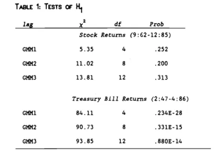
H is implied, for instance, by constant real interest rates as assumed by Hall (1978). For a different specification of preferences, this hypothesis has recently been tested by Christiano, Eichenbaum, and Marshall (1990) using methods similar to those discussed in this paper to account for temporal aggregation. Ignoring (3.8), fl is exactly identified by the least-squares normal equations (3.10). To test H we make the simplifying assumption that E(e+2IJt) — 0, which permits us to use the least-squares inference methods suggested by Hansen and Hodrick (1980).

The tests statistics for H are reported in Table 1 for three choices of lag. The column labeled x2

gives

the test st.tistic, which is distributed asymptotically as a chi-square with df degrees of freedom and probability

value Prob. The results for stock returns indicate that there is little evidence against H. This finding is consistent with the large standard errors for

reported

in previous studies and subsequently here for stock return equations. In contrast, there is substantial against H when Treasury bill returns are studied.

Next it is of interest to examine and Pq separately. Recall that satisfies the restriction (3.8): loPc —

Pq

When is zero, it follows that

(4.2)

H2: Pq —

0.

That is, temporally aggregated returns are not predictable given x.

Alternatively, since —

(4.3) _H3: —

0.

Equivalently, the growth rate of temporally aggregated consumption is not

predictable given x. Hypothesis H2 is consistent with linear utility while hypothesis H3 is consistent with an intertemporal elasticity of substitution equal to zero. One of our motivations for looking at H3 is Hall's recent finding that (l/7) is approximately zero. Hall's finding is in contrast to our earlier results [Hansen and Singleton (1982, 1983)] from a model in which the sampling interval of the data coincided with the decision interval of

agents.

So far we have examined hypotheses based on two extreme cases of proportionality restriction (3.8).

We now consider the more general

hypothesis:

(4.4)

H4: c —

Pq for some v

in

.

We test this hypothesis using the minimized value of (3.11) with W — W, which

is asymptotically distributed as chi square with lag - 1 degrees of freedom (Hansen 1982). The reduction in degrees of freedom by one relative to the

test statistics for hypotheses H2 and H3 occurs because y is no longer specified a priori, but is now estimated. While the derivation in Hansen (1982) relies on the assumption that E(e+2IJ) —

0,

in the appendix we show that the weaker assumption E(Et+2IJt) —

0

suffices, where Et+2 —

Estimates

of y and the chi-square statistics for testing H2, H3, and

H4 using stock return data are reported in Table 2.

The chi-square statistics indicate that there is little evidence against H2, but somewhat

more evidence against H .

Since

H is less restrictive than H ,

there

is

3 4 2

also little evidence against H. The estimate of _{y, is not very precise,} and in fact has the wrong sign. The last column of the table labeled corr

reports the estimated correlation of which should be .25. In all cases it is close to this magnitude.

Further insight into the sample information about y is provided in Figure 1. This figure was constructed by solving the optimization problem

(3.11) repeatedly, holding y fixed at values along the horizontal axis. In all cases W was set to W. The vertical axis displays the corresponding values of the criterion functions evaluated at the solutions to these problems. Each curve represents a different choice of lag. The minimum value of each curve- -

i.e.,

the statistic used to test H- -

occurs

at the y reported in Table 2. For y equal to the minimized value of the GM/I criterion function has an asymptotic chi square distribution with 2(lag) degrees of freedom. As already noted, there is a loss of one degree of freedom when y is set to y.

While the point estimates of are positive, the three curves in Figure 1 indicate that values of less than zero are plausible. Another interesting feature of these curves is that they all peak at values of 7 near -20 before asymptoting to the values at ii = reported in Table 2. These findings are consistent with the small values of y reported in Hansen and

Singleton (1982,1983). In contrast to Hall (1988), accounting for temporal aggregation does not lead us to conclude that larger values of _(smaller values of 1/171) are more plausible than values of y close to zero.

In the case of Treasury bill returns, there is substantial evidence against all of the null hypotheses H, H, and H, especially for lag equal to two and three. In contrast to equity returns and consistent with our

discussion in section 2, the estimated first-order autocorrelation of t+2 not close to .25. The fact the estimated autocorrelations of the bond

disturbances differ substantially from .25 suggests that the incorrect imposition of the restriction p — .25 may induce important biases in the

estimates of parameters or standard errors. While the point estimates for have the wrong sign, it is difficult to interpret these coefficients in light of the pervasive evidence against hypothesis H4.

More efficient, system estimates of can be obtained using the system GMM and ML methods described in section 3. In calculating these estimates. we focus on the stock return data because of the large values of the chi square statistics reported in Table 3 for the Treasury bill data. The rows labeled OGMM1ag. with lag —

1,

2, and 3, in Table 4 display the estimates of and the chi square statistics for the hypotheses H2, H3, and H4 from fitting (3.9) subject to the restriction (3.8) using the moment conditions (3.20). Estimated standard errors and probability values of the chi-square statistics are in parentheses. The estimated autocorrelations (corr) of —

[-y l]e [the disturbance in (2.9)] are reported in the last column of the table. Comparing the OGMM results in Table 4 with the corresponding GMM results in Table 2, there are small gains in precision in using OGMM system estimation. Also, the test statistics are similar across the two tables.

The ML estimates displayed in rows MLlag in Table 4 zere obtained using parameterization (3.23) and (3.24), where lag determines the orders of the lag polynomials A(L) and 8(L). We used a parameterization of 8(ç) suggested in Monahan (1984) to insure that the zeros of this scalar polynomial are outside the unit circle of the complex plane. To evaluate the Gaussian likelihood function, we used the filtering methods described in Anderson and Moore (1979) and Hansen and Sargent (1990). The ML estimates have smaller

estimated standard errors than both the CNN and CC/IN estimates. Also, the associated likelihood ratio tests provide somewhat more evidence against the hypothesis 113

—

Comparing Tables 2 and 4, recall that the CMII estimates based on the moment conditions (3.10) (Table 2) are consistent and the inference procedures are valid whether or not the true AR/IA representation for is (3.9) with E(e+2IJ) —

0.

In contrast, the efficiency of the OGMM and ML estimates displayed in Table 4 relies on a correct specification of the time series law of motion for Also, the OGMM and ML estimates were obtained using different probability models, which may help to explain the apparent gain in precision in using ML over OGMM.

Up to this point, we have presumed that the correlation restriction (3.19) implied by the ICAPMs for stock returns in section 2 are not imposed in estimation using GM/I or ML procedures. Estimator efficiency can, in general, be increased by imposing the unconditional correlation restriction (3.19) along with the moment restrictions implied by (2.11). The first three

rows of Table S display the GM/I estimates of y based on the moment

conditions (3.10) and (3.19). These estimates were calculated using the heteroskedastic-consistent weighting matrix described in Hansen (1982) in

order to accommodate two potential sources of heteroskedasticity. First the

original disturbance 6t+2 might be heteroskedastic as in the model

non-expected utility model. Additional heteroskedasticity is introduced into

2

the moment equations through the disturbance u÷2 —

25t+2

6t÷26t+l used in (3.19) to impose the correlation restrittion. The validity of this estimation for the non-expected utility model relies on the assumption that the value-weighted return is also the return on the wealth portfolio (see

H with the correlation restriction added.

The most striking feature of the GMM results in Table 5 is that the estimated standard errors are reduced dramatically over those displayed in Table 2. At the same time, adding the correlation restriction to the set of moment conditions leads to comparable point estimates, since this restriction is almost satisfied in Table 2. It is still true that there is little evidence against the hypothesis that

—

0.

The last three rows of Table 5 display ML results with the correlation restriction (3.19) imposed on the law of motion (3.23). In contrast to Grossman, Melino, and Shiller (1987), this restriction was imposed directly on the discrete time law of motion for (ye) rather than indirectly through a continuous time specification of the expected utility model. A potential advantage of focusing on the former is that we avoid the aliasing problem of identifying a continuous time probability law from discrete time data. Since homoskedasticity was imposed, these estimates relate to the expected utility

model. The ML results are comparable to the GMII results: the ML estimates of in Tables 4 and 5 are similar but the standard errors are notably smaller in Table 5.

Finally, Table 6 displays the population efficiency bounds associated with the various estimators.

The column headings refer to the six

probability models in Table 4, with the parameters taken to be the point estimates obtained under H. For each of these probability models and each

choice of lag, the single-equation efficiency bound, 11ag' for the CMII estimator based on the moment conditions (3.3) was calculated. To make this bound comparable to the estimated standard errors we divided it by 278 and took square roots. The row labeled lag — is computed using inf given by (3.17). The efficiency bounds

were

calculated using the recursive methods

described in Hansen and Singleton (1989) and GAUSS code written by John Heaton and Masao Ogaki.

In section 3 it was noted that, as lag 4

c 1fl1ag

converges to the single-equation efficiency bound for the model (2.9) with the moment conditions (2.11) imposed, ln.f.

From Table 6 it is seen that this

convergence is very rapid for the model of stock returns with the law of motion (3.9). This is consistent with our findings in Tables 2 and 4 that

there are no notable gains in precision from using OGMM instead of GMM estimation.

Convergence is slower for the parameterization (3.23). In the cases of ML1 and ML2, the estimates of the law of motion (3.23) predict much larger values of the standard errors than we found in practice in Table 2. On the other hand, ML3 predicts standard errors very similar to those reported in Table 2 for small values of lag. The lag — bounds reported in Table 6 for

all three ML runs are similar to the estimated standard errors reported in Table 4 for the corresponding ML estimates.9 This means that the efficiency of the system ML estimators can be attributed largely to their selection, at least implicitly, of efficient instruments rather than to their exploitation of the information about the order of the full ARMA model.

We

draw three conclusions

from these results. First, the estimated efficiency gains are aensitive to the choice of probability model for stock return and consumption data. The calculations with the ML3 model seem to replicate most closely our estimated standard errors for GMM and ML estimators of . Second, this probability model implies substantial gains in precision from exploiting the orthogonality conditions associated with the entire history of y. These gains are related to the location of the roots of the moving average polynomial. For the ML parameterizations there are

complex roots near the unit

circle

(see Hansen and Singleton (1989)]. Third, there seems to be very little efficiency gain to implementing the efficient system estimator instead of the efficient single-equation estimator.

Finally, we investigated the impact on asymptotic efficiency of imposing the the correlation restriction. Hansen, Heaton, and Ogaki (1988) characterized GMM efficiency bounds for general forms of multi-period conditional moment restrictions, and Heaton and Ogaki (1988) presented an

algorithm for computing an efficiency bound that incorporates a conditional moment restriction. Single-equation efficiency bounds that incorporate the

conditional moment restriction are displayed in the last row of Table 6. As was anticipated by the estimates in Table 5, there is a notable efficiency

V. CONCLUSIONS

In this paper we have accomplished the following. First we have investigated the extent to which the serial correlation restriction derived by Working (1960) for temporally aggregated Brownian motions apply to log-linear asset pricing models. We find that this restriction is not as pervasive as was previously thought. For instance, while the correlation restriction may be applicable to equities returns, it is not applicable to bond returns, except in two limiting cases: long term bonds or returns constructed by rolling over a large number of short term bonds. Second, we showed that when applicable, the serial correlation restriction can improve substantially the efficiency of estimators of the preference parameter Third we proposed two new GMM-type estimators. One of these estimators is asymptotically equivalent to the finite-lag efficient, single equation GM/I

estimator, but is constructed to be insensitive to the choice of

normalization. The other estimator is a fully efficient system estimator for

models in which the observed time series can be characterized as a

multi-period counterpart to a finite-order vector autoregression. Fourth, we provide statistical evidence showing that smaller (absolute) values of the preference parameter are more plausible than larger ones for equity data.

For bond data,

however, we found substantial evidence against the

restrictions implied by the model. This evidence is consistent with our previous empirical results, Hansen and Singleton (1982,1983), some of which did not accommodate time aggregation in consumption.

In this paper we have followed much of the theoretical and empirical

literature on continuous time IGAPM's by modeling preferences as time separable. In taking continuous time limits, however, it may be more plausible to introduce local durability so that consumption at near-by points

in time are close substitutes. Recently, Hindy and Huang (1989) have investigated theoretical continuous time ICAPM's with local durability. Such models may

be

better suited for analyzing the

effects

temporal aggregation

NOTES

1. Often the conditional moment restrictions are all that is known by the

econometrician about the distribution of the errors; in particular, the

family of distributions from which the errors are drawn is unknown.

2. The null hypotheses that risk premia are zero or constant can be expressed as restrictions on conditional forecasts of excess holding period returns. This observation underlies many of the tests of expectations theories of the term structure of interest rates, as well as tests of whether forward exchange rates are optimal forecasts of future spot exchange rates [e.g., Hansen and Hodrick (1980)). Similarly, recent studies of mean reversion in asset returns examine whether continuously compounded, multi-period returns have constant conditional means (e.g., Fama and French (1988)).

3. We are also ignoring the implication of a monetary econony that the prices of nominal discount bonds should be less than or equal to one.

4. For a given value of y, optimization problem (3.11) is quadratic and can be solved by simple matrix manipulations. Hence the estimate of y can be computed by first concentrating out all of the parameters for each and then doing a one-dimensional numerical search over y.

5. The fact that this estimator of y is not sensitive to normalization is no

guarantee that its finite sample behavior will dominate thst of the

asymptotically equivalent single equation GMM estimators.

past values of as well. Because of the linearity we presumed in the underlying estimation environment, there would be no efficiency gain associated with using such indices. It is still possible that linear forms of conditional moment restrictions such as (3.2) may exist even though the complete law of motion for y is nonlinear. In these circumstances, there may well be efficiency gains to using nonlinear functions of current and past values of y as indices.

7. The formal large sample justifications for using approximate time series models typically have the specification of the approximate model depend explicitly on sample size with the idea that more general models are fit with larger sample sizes. In this manner the approximation error is avoided asymptotically.

8. The monthly, temporally aggregated returns were derived by constructing monthly returns from daily data and then averaging the monthly returns over the days of the month. The monthly returns were constructed such that the monthly average involved daily returns from only the current and previous

months.

9. The asymptotic variance of the ML

estimator

of y

should

be less than or equsl to inf.

In

comparing Tables 4 and 6, we see that this ordering is actually reversed. This occurs because of the different methods used to estimate the asymptotic variance and irif. We used the inverse Hessian to construct an estimate of the asymptotic variance, and we used the estimated parameter values in conjunction with recursive formulas reported in Hansen and Singleton (1989) to construct an estimate of in.f.

TABLE 1: TESTS OF H1 2

lag

x

df

Prob Stock Returns (9:62-12:85) GMM1

5.35

4

.252

CMM2

11.02

8

.200

GMM3

13.81

12 .313

Treasury Bill Returns (2:47-4:86)

GMM1 84.11 4 .234E-28

GMM2

90.73

8 .331E-15

TABLE 2: GMM ESTIMATION FOR SToCKS

(9:6212:85)

x2tdl

-y H H H lag

o

2 3 4 cerr 1 1.73 0.26 [2] 4.54 [2] 0.07 [1] .266 (4.19) (.878) (.103) (.792) 2

2.14

0.73 [4]

8.85 [4]

0.38 [3]

.254

(3.82)

(.947) (.065 (.945) 3 3.05 2.46 [6] 9.10 [6] 1.71 [5] .231 (3.68) (.872) (.168) (.887)

TABLE 3: GMM ESTIMATION

FoR Bot-.ios (2:474-:86)

2

x [df]

H H H lag o 2 3 4 corr 1

11.61

80.90 [2]

1.04 [2]

0.36 (1]

.135

(14.25) (.2E-17)

(.594)

(.547)

2

11.36

72.80 [4] 18.74 [4] 18.12 [3]

.150

(13.48) (.5E-14)

(.001)

(.0004)

3

8.59

73.98 [6] 21.30 [6] 20.27 [5] .154

(7.85) (.6E-13)

(.002)

(.001)

TABLE 4: EFFICIENT SYSTEM ESTIMATION (9:6212:85)

x2[df]

H H H lag

o

2 3 4 corr OGMM1

1.01

0.10 [2]

6.17 [2] 0.01 [1] .275 (3.24) (.950) (.046) (.943) OGMM2 1.94 0.49 [4] 8.41 [4] 0.18 [3] .258 (3.62) (.974) (.077) (.981) OG!*f3 2.14 1.42 [6] 9.48 [6] 1.01 [5] .252 (3.31) (.964) (.149) (.962) ML1 2.25 3.87 [4] 11.91 [6] 2.69 [3] .253 (2.26) (.424) (.018) (.442) ML2 2.40 4.23 [6] 13.78 [6] 2.78 [5] .245 (2.22) (.631) (.032) (.733) ML3 2.28 5.80 [8] 15.33 [8] 4.43 [7] .245 (2.16) (.670) (.053) (.729)

TABII 5: ESTIMATION WITH CORRELATION RESTRICTION (9:62-12:85)

lag

df Prob GMM1

2.24

0.09

₂

.954

(1.73)

GMM2 2.17

0.31

4

.989

(1.73)

GMM3

2.10

1.38

6

.967

(2.20)

ML1 2.30

2.69

4

.610

(1.53)

ML2 2.29

2.78

6

.835

(1.42)

ML3 2.17

4.43

8

.816

(1.41)

T&BLE 6: EFFICIENCY BOUNDS

Model

OGMM1 OGMM2 OGMM3 ML1 ML2 ML3

Lag

1

3.29

4.19

4.24

12.30

6.10

4.28

2

3.16

3.63

3.83

7.01

4.35

3.81

3

3.15

3.59

3.31

5.80

4.31

3.79

4

3.15

3.59

3.28

5.08

4.19

3.68

5

3.15

3.59

3.28

4.62

3.71

3.40

10

3.15

3.59

3.28

3.57

3.07

2.89

20

3.15

3.59

3.28

2.90

2.67

2.56

40

3.15

3.59

3.28

2.49

2.37

2.29

3.15

3.59

3.28

2.03

1.98

1.93

correlation restriction

2.46

1.85

1.76

1.47

1.36

1.33

LLLOL6

L 9 c

4v

£

0

RZPKRENCES

Amemiya, T., "The Maximum

Likelihood

and Nonlinear Three-stage Least Squares Estimator in the General Nonlinear Simultaneous Equations Model,' Econometrics 45, 1977, 955-968.

Anderson, B. D.O., and J. B. Moore, Optimal Filtering, Prince-Hall, Inc. Englewood Cliffs, New Jersey, 1979.

Barro, R.J. , 'On the Predictability of Tax-Rate Changes,' manuscript, University of Rochester 1981.

Breeden, D., "Consumption, Production, and Interest Rates: A Synthesis," Journal of Financial Economies 16, 1986, 3-39.

Christiano, L., M. Eichenbaum and D. Marshall, "Permanent Income Model Revisited," forthcoming in Econometrics, 1990.

Cox, J., J. Ingersoll and S. Ross, "A Theory of the Term

Structure

of Interest Rates," Econometrica 53, 1985, 385-408.

Duffie, D. and L. Epstein, "Stochastic Differential Utility and Asset Pricing," manuscript, Stanford University, 1989.

Dunn, K. D., and K. J. Singleton, "Modeling the Term Structure of Interest Rates Under Nonseparability of Preferences and Durability of Goods," Journal of Financial Economics 17, 1986, 27-55.

Epstein, L. and S. Zin, "Substitution, Risk Aversion, and the Temporal Behavior of Consumption and Asset Returns: A Theoretical Framework,' Econometrics 57, l989a, 937-969.

Epstein, L. and S. Zin, "Substitution, Risk Aversion, and the Temporal Behavior of Consumption and Asset Returns II: An Empirical Anaysis, manuscript, University of Toronto, l989b.

Fama, E., and K. French, "Permanent and Temporary Components of Stock Prices," Journal of Political Economy 96, 1988, 246-273.

Ferson, W., "Expectations of Real Interest Rates and Aggregate Consumption: Empirical Tests," Journal of Financial and Quantitative Analysis 18, 1983, 477-497.

Grossman, S., A. Melino and R. J. Shiller, "Estimating the Continuous Time Consumption-Based Asset Pricing Model," Journal of Business and

Economic

Statistics 5, 1987, 315-327.

Hall, R. E., "Intertemporal Substitution and Consumption," Journal of Political Economy 96, 1988, 339-357.

Hansen, L.P., "Large

Sample

Properties of Generalized Method of Moments Estimators," Econometrics 50, 1982, 1029-1054.

Hansen, L.P., "A Method for Calculating Bounds

on

the Asymptotic Covariance Matrices of Generalized Method of Moments Estimators," Journal of

Econometrics, 30, 1985, 203-238.

Hansen, L.P., "Semi-Parametric Efficiency Bounds for Linear Time Series Models," manuscript, University of Chicago, 1989.

Hansen, L.P., J. Heaton and M. Ogaki, "Efficiency Bounds Implied by Multiperiod Conditional Moment Restrictions," Journal of the American Statistical Association 83, 1988, 863-871.

Hansen, L.P., and R. J. Hodrick, "Forward Exchange Rates as Optimal Predictors of Future Spot Rates: An Econometric Analysis," Journal of Political Economy 88, 1980, 829-863.

Hansen, L.P., and R. J. Hodrick, "Risk Averse Speculation in the Forward Foreign Exchange Market: an Econometric Analysis of Linear Models," in

J. Frenkel ed., Exchange R