Indirect Estimation of Long Memory Volatility Models
Nigel Wilkins
School of Finance and Economics University of Technology, Sydney
PO Box 123 Broadway NSW 2007 Australia Ph: 61 2 95147784 Fax: 61 2 95147711 [email protected] January 2004 Abstract
An indirect estimator is proposed for two long memory volatility models; the fractionally integrated generalised autoregressive conditional heteroskedasticity (FIGARCH) model and the long memory stochastic volatility (LMSV) model. The small sample properties of the indirect estimator are compared to the small sample properties of conventional maximum likelihood estimators. It is found that the indirect estimator has the potential to perform favourably with respect to maximum likelihood for higher order parameterised FIGARCH and LMSV models.
Keywords: Fractional Integration, Persistence, Simulation.
1
Introduction
Recent empirical research examining the time dependent conditional variances of financial variables has found that long memory is a relevant factor to be taken into consideration; see for example, Ding, Granger and Engle (1993), Ding and Granger (1996), Bollerslev and Mikkelsen (1996), and also Engle and Bollerslev (1986) for the original contribution on infinitely long memory conditional variances. This evidence of long range behaviour has lead to the development of integrated models for conditional variance. Under the restrictive integer framework, a stationary volatility process for a financial asset (where the level of integration isd= 0) exhibits exponential decay in response to an exogenous shock, while a nonstationary volatility process (whered= 1) displays no tendency to revert to its unconditional volatility, or variance, after an exogenous shock and actually retains some permanent component. In a manner similar to that for the conditional mean, it has been found that thisd= 0,1 dichotomy imposes too heavy a restriction on the allowable behaviour of the conditional second moment of a time series. Rather than restricting attention to integer levels of integration, it seems sensible to allow a compromise between the stationary models of conditional variance and nonstationary or integrated models. For the conditional mean, this has lead to the development and popularisation of the autoregressive fractionally integrated moving average (ARFIMA) model due to Granger and Joyeux (1980) and Hosking (1981); see also Baille (1996) for a survey of developments in ARFIMA modelling.
A natural framework on which to build a fractional model for the conditional variance is the autore-gressive conditional heteroskedasticity (ARCH) model due to Engle (1982) or the generalised ARCH (GARCH) model due to Bollerslev (1986). Both models have received extensive application in mod-elling the time varying properties of the conditional variance of financial time series; see Bollerslev, Chou and Kroner (1992) or Bollerslev, Engle and Nelson (1994) for a review of ARCH models. Baille, Bollerslev and Mikkelsen (1996) propose the fractionally integrated GARCH (FIGARCH) model and a time domain maximum likelihood (TDML) estimator for the parameters in this model. Alterna-tively, the stochastic volatility (SV) class of models, see Taylor (1994) for a survey, can be utilised as a framework on which to build a fractional model. Harvey (1993) was the first to consider this by specifying a fractional noise process to drive the long memory component of the SV model. Breidt, Crato and deLima (1998) propose the long memory stochastic volatility (LMSV) model and a frequency domain based maximum likelihood (FDML) estimator for the parameters in this model. Unfortunately, the maximum likelihood estimators for the FIGARCH and LMSV models have potential problems in their application. The TDML estimator for the FIGARCH model has truncation and starting value problems, while the FDML estimator for the LMSV model can be prone to sizeable finite sample bias problems. This paper overcomes these estimation problems by proposing an indirect estimator for the two models based on the Gorieroux, Monfort and Renault (1993) version of the indirect estimator. The
indirect estimator has already received application to fractional models for the conditional mean of a process; see Martin and Wilkins (1999) for details.
The outline of the paper is as follows. Section 2 briefly reviews models for conditional variance. Section 3 develops an indirect estimation procedure for FIGARCH and LMSV models by discussing alternative auxiliary models that may be implemented, computationally efficient simulation procedures and an estimation algorithm for empirical application. Section 4 reports the results of a set of simulation experiments to compare the small sample properties of the maximum likelihood and indirect estimators. Section 5 concludes.
2
Models for Conditional Variance
Consider some time seriesRt with conditional mean equation
Rt=f(xt) +σtεt (1)
where, in very general terms,f(xt) denotes some functional form of the explanatory variables xt,σt is
the time varying conditional standard deviation (variance) andεtis iid(0,1). Assuming the specification f(xt) =µtwhereµtis the conditional mean ofRt, then (1) can be expressed as the (conditional) mean
corrected series
rt=Rt−µt=σtεt (2)
where the time series rt is now a white noise (WN) process.
2.1 Autoregressive Conditional Heteroskedasticity
The process rt exhibits ARCH(q) effects ifσt can be written
σt2 =ω+α(L)rt2 (3) whereωis a positive constant andα(L) =Piq=1αiLi is a lag operator polynomial inLwith allα
i
non-negative to ensureσ2
t is positive for all possible realisations ofrt. When the appropriate specification
for (3) includes laggedσ2
t, the model becomes the generalised ARCH(p, q), or GARCH(p, q) model due
to Bollerslev (1986)
σ2t =ω+α(L)r2t +β(L)σ2t (4) where β(L) = Ppi=1βiLi is a lag operator polynomial in L with, once again, all βi non-negative to
ensureσ2
t is always positive. Bollerslev (1986) shows that (4) can be rearranged to give
wherevt=r2t−σ2t is a random shock, or error component in conditional variance and (5) is interpreted
as being an ARMA(q∗, p) model for r2
t where q∗ = max{p, q}.
Engle and Bollerslev (1986) extend (5) by allowing 1−α(L)−β(L) to contain a unit root, giving the integrated GARCH(q∗, p), IGARCH(q∗, p) model
Π(L)(1−L)ε2t =ω+ [1−β(L)]vt (6)
where Π(L) = (1−L)−1[1−α(L)−β(L)] = (1−L)−1[1−Φ(L)] is of order q∗−1; see also Nelson (1990). In practical application, d= 1 has been found to be a suitable parameterisation for this class of model. The two GARCH extremes represented in (4) and (6) might be considered too rigid to approximate the sensitive dynamics in the data generating process (DGP) of a financial time series accurately. This suggests the relevance of more general, fractionally integrated, versions of these models. This is advantageous because incorporating fractional integration into the conditional second moment of a time series allows the conditional variance function to display persistent but still mean reverting behaviour. This appears to be more consistent with actual financial returns data than that behaviour captured in thed= 0 ord= 1 models.
The fractionally integrated GARCH, or FIGARCH model due to Baille, Bollerslev and Mikkelsen (1996) overcomes the restrictions of these models. The FIGARCH model is obtained by using the fractional differencing operator in (6) rather than the integer differencing operator. The model now becomes
Π(L)(1−L)drt2=ω+ [1−β(L)]vt (7)
which is in its ARMA(q∗, p) representation forr2
t and the fractional differencing filter is as
convention-ally defined
(1−L)d= (j−d−1)!
j!(−d−1)!L
j (8)
for j = 1,2, . . . ,∞. Rearranging (7) results in an alternative expression for the FIGARCH(p, d, q∗) model
σ2t =ω+β(L)σt2+h1−β(L)−Π(L)(1−L)dir2t (9) which shows howσ2
t evolves over time. In an analogous fashion to the exponential GARCH model of
Nel-son (1991), Bollerslev and Mikkelsen (1996) extend (7) to the fractionally integrated EGARCH(p, d, q∗), or FIEGARCH(p, d, q∗) model. The FIGARCH model has been applied to stock market returns data by Bollerslev and Mikkelsen (1996) and Psaradakis and Sola (1995)
As an illustration, the specific formulation for the FIGARCH(1, d,1) model is
σ2t =ω+β1σ2t−1+
h
1−β1L−(1−π1L)(1−L)d
i
where π1 =α1 +β1 is as defined in reference to (6). Equation (10) can be expressed as the
observa-tionally equivalent infinite order ARCH representation
σt2 = ω 1−β1 + " 1− (1−π1L)(1−L) d (1−β1L) # rt2= ω 1−β1 +λ1(L)r 2 t (11)
where λ1(L) = P∞i=1λ1,iLi. Similarly, the FIGARCH(1, d,0) model is obtained by setting π1 = 0 in
(10) σt2=ω+β1σt2−1+ h 1−β1L−(1−L)d i r2t (12)
and this has the observationally equivalent infinite order ARCH representation
σt2= ω 1−β1 + " 1− (1−L) d (1−β1L) # rt2= ω 1−β1 +λ2(L)r 2 t (13) where λ2(L) = P∞
i=1λ2,iLi. Following Bollerslev and Mikkelsen (1996), the ARCH coefficients in the
lag operator polynomialλ1(L) have the recursive form
λ1,i=π1−β1+d (14) fori= 1 and λ1,i=β1λ1,i−1+ · (i−1−d) i −π1 ¸ δi−1 (15)
for i = 2,3, . . . and where δi = δi−1(i−1−d)/i is a recursive function for the coefficients in the
expression for (1−L)d in (8). The coefficients in the lag operator polynomial λ2(L) are found by
setting π1 = 0 in (14) and (15). The two FIGARCH models in (10) and (12) are used as alternative DGPs for the Monte Carlo experiments in Section 4.
Estimation of the conventional GARCH model is nontrivial, although straightforward, because of the restrictions on the model coefficients to ensure conditional variance is always positive. In the case of the FIGARCH model, this complexity is increased because negative coefficients in the differencing filter in (8) cannot be avoided. This implies the simplest class of model for long memory conditional variances, the FIGARCH(0, d,0) model is not defined because the resulting negative coefficients in (9) cannot be avoided. For the more general FIGARCH(p, d, q∗) model, a general expression for the required parameter restrictions is not yet available, but, as Bollerslev and Mikkelsen (1996) note, the restrictions necessary for specific FIGARCH(p, d, q∗) models can be obtained on a case by case basis. For the FIGARCH(1, d,1) model, these are
β1−d≤π1≤ (2−3 d) (16) and d · π1− (1−d) 2 ¸ ≤β1(π1−β1+d) (17) which simplify to 0< β1 < d <1 (18) for the FIGARCH(1, d,0) model.
2.1.1 Time Domain Maximum Likelihood Estimation
By assuming conditional normality, it is possible to estimate (9) by maximising the natural logarithm of the conventional ARCH likelihood function
lnL{Θ1;r2t}=− 1 2ln(2π)− 1 2 T X t=1 " lnσt2+ rt2 σ2 t # (19) where Θ1 = {d, ω, β1, β2, . . . , βp, π1, π2, . . . , πq∗} is the FIGARCH parameter vector, rt2 is obtained
using the conditional mean equation and σ2
t is obtained approximately according to (9) by using the
fractional differencing filter truncated at some point beyond which the contribution of extra terms in the summation is negligible. Estimation of the FIGARCH model using (19) is referred to as time domain maximum likelihood (TDML) estimation.
Three points should be noted about this TDML estimator. First, the truncation of the differencing filter means that maximum likelihood estimation is approximate only, although the extent of the approximation can be reduced by increasing the truncation point. This procedure is therefore not an exact estimator like the TDML estimator for the parameters of the ARFIMA(p, d, q) model for the conditional mean; see Sowell (1992a). Second, because of the truncation, estimation using (19) can be expensive in small samples. Although this might not be too much of a concern when using financial data sets, it still involves the loss of sample data and therefore sample information. Third, the truncation means the actual series being used is not the true fractionally differenced series and therefore there is a bias being introduced into the estimation procedure. This can be justified using an argument similar to that in Sowell (1992b) when discussing the estimation of the parameters in the conditional mean equation with an approximate TDML estimator.
Estimation using (19) is often referred to as quasi maximum likelihood (QML) estimation because the assumption of a normally distributed error process does not always hold in financial data sets. Using a robustified estimator of the covariance matrix of the parameter estimates is asymptotically valid however, see Weiss (1986) and Bollerslev and Wooldridge (1992). A heteroskedasticity consistent covariance matrix can be obtained using
H(Θb1)−1G(Θb1)H(Θb1)−1 (20)
whereG(Θb1) is the outer product of the gradients andH(Θb1) is the hessian, both of which are evaluated atΘb1.
2.1.2 Frequency Domain Maximum Likelihood Estimation
The ARMA representation of the FIGARCH model in (7) allows the model to be estimated using a frequency domain based likelihood function. The interpretation of (7) as an ARFIMA(q∗, d, p) model for the squared errors allows standard time series results to be used to obtain the spectrum forrt2. In its most general form, the spectrum is
Ir2(λ) = σ 2 ν 2π |Π(e−iλ)|2 |β(e−iλ)|2 ¯ ¯ ¯1−e−iλ¯¯¯−2d (21) where |Π(e−iλ)| and |β(e−iλ)| are the spectral generating functions corresponding to the lag operator
polynomials Π(L) andβ(L), andλis angular frequency.
Equation (21) now allows specification of the spectral likelihood function, see Fox and Taqqu (1986), lnL{Θ1;p(λj)}=− 1 2π T /2 X j=1 p(λj) Ir2(λj) (22)
where Θ1 is the parameter vector defined in reference to (19),λj = 2πj/T forj = 1,2, . . . , T /2 is the jth Fourier frequency and p(λj) is the estimated periodogram for the squared data. Once estimates
for the parameters in the lag operator polynomials in the ARFIMA representation in (7) have been obtained, they can be used to generate an estimate of the constantω, and all parameters can then be substituted into (9) to obtain the more familiar ARCH specification of the model. Estimation using (22) is advantageous because it avoids the restrictions inherent in the TDML procedure.
2.2 Stochastic Volatility
The ARCH class of models explain the conditional variance as a function of (squared) past errors, thus imposing dependence between rt and σt2. An alternative to this is the SV model, which specifies a
DGP forσ2
t that is independent of rt. The SV model can be written σ2t =σ2exp(νt
2)
2 (23)
where νt is some process that imposes the heteroskedasticity inσ2
t and that is also independent ofrt.
Most simply, νt can be taken to be an AR(1) process, νt =φ1νt−1+ηt, with the normal requirement that |φ1|<1 for stationarity to hold. An alternative fractionally integrated DGP for the conditional
variance is considered by Harvey (1993) and extended by Breidt, Crato and de Lima (1998). The equation explaining the evolution of the conditional variance is given the specification
σt=σexp(νt
where nowνt follows the ARFIMA(p, d, q) process
Φ(L)(1−L)dνt=δ+ Θ(L)ςt (25)
where Φ(L) =Ppi=0φiLi, Θ(L) =Pqi=0θiLiandςtis WN(0, σ2ς). The long memory stochastic volatility,
or LMSV(p, d, q) model is defined by the specification of the ARFIMA model in (25).
Following Breidt, Crato and de Lima (1998), the natural logarithm of the square of (2) with (24) substituted in can be rearranged to give
ln(rt)2 =E[lnε2t] +νt+²t (26)
where ²t = lnr2t −E[lnrt2] is an iid(0, σ²2) error process. Using (26), the persistence in conditional
variance nature of the series can now be examined using conventional ARFIMA methods. As a direct extension of (21), the spectrum of (26) is
Ir2(λ) = σ2 ς 2π |Θ(e−iλ)|2 |Φ(e−iλ)|2 ¯ ¯ ¯1−e−iλ¯¯¯−2d+ σ²2 2π (27)
which can be found directly by invoking the linearity property of the spectrum. As an example, the simplest model that can be considered is the LMSV(0, d,0) model
rt=σexp ( (1−L)−dς t 2 ) εt (28)
while a more general specification is the LMSV(1, d,1) model
rt=σexp ( (1−φL)−1(1−L)−d(1 +θL)ς t 2 ) εt (29)
Both of these models are used in Section 4 as alternative DGPs for the Monte Carlo experiments. An advantage of the LMSV model is that the restrictions on the parameters in the FIGARCH model are not present, see (16) to (18), and the simplest fractional model for conditional variances withp, q= 0 butd6= 0 can now be considered.
2.2.1 Frequency Domain Maximum Likelihood Estimation
Estimation of the SV model using TDML procedures requires numerical integration at each observa-tion; see for example Gourieroux, Monfort and Renault (1993). A frequency domain based likelihood function specified using (27) avoids this problem. From Breidt, Crato and de Lima (1998), the spectral representation of the likelihood function for the transformation of the LMSV model in (26) is
lnL{Θ2;p(λj)}=−2Tπ T /2 X j=1 " lnIr2(λj) + p(λj) Ir2(λj) # (30)
where Θ2 ={d, φ1, φ2, . . . , φp, θ1, θ2, . . . , θq, σς2, σ²2}is the LMSV parameter vector andp(λj) is now the
estimated periodogram for the natural logarithm of the squared mean corrected data. Estimation of the LMSV model using (30) is referred to as frequency domain maximum likelihood (FDML) estimation. Breidt, Crato and de Lima (1998) show the strong consistency of the estimates obtained using (30). The convenient spectral representation of fractional processes and the truncation involved in maximising (19), implies that maximisation of (30) has the potential to be computationally easier and more accurate than (19).
3
Indirect Estimation
3.1 The Indirect Estimator
At its most elementary level, the indirect estimator obtains parameter estimates for one model by estimating the parameters of another model. The estimation procedure has two basic requirements. The first is that the direct model of interest, that is the model the empirical researcher wishes to estimate, must be easy and computationally efficient to simulate. This model of interest is never actually “directly” estimated, only simulated. The second requirement is that there exists some indirect, or auxiliary model that is straightforward to estimate and that can be considered to be representative of the direct model of interest. The parameter estimates for this auxiliary model are of no interest in their own right. Indirect estimation yields consistent parameter estimates for the direct model by comparing the estimates of the auxiliary model obtained using the actual data to those obtained using artificial data simulated from the direct model. The direct model is then repeatedly simulated within an iterative routine until the parameter estimates for the auxiliary model obtained using the actual data and the simulated data are equal, or sufficiently close. The set of parameters for the direct model used to generate the last simulated series of numbers are the indirect parameter estimates for the direct model.
Martin and Wilkins (1999) consider estimating the parameters in the general ARFIMA(p, d, q) model using simple AR(p) processes as auxiliary models. As a specific example, denote the autoregressive parameter vector in an AR auxiliary model asρ, and the estimate of ρobtained using the actual data as ρ(a). Now denote the parameter vector for the direct model in (25) as Ψ = {d, δ,Φ(1),Θ(1), σ2}.
Indirect estimation involves simulating (25), for a particular set of parameter values, say Ψ1, and then
estimating the AR auxiliary model with this simulated series. Denote the estimate of the auxiliary model parameter using this simulated series asρ1(s). Then, intuitively, the indirect estimator of Ψ is
that Ψi corresponding to theith simulated series where
with a satisfactory tolerance level prespecified. When the dimension of the parameter vectors Ψ and
ρ are the same, the criterion simplifies to ρi(s) = ρ(a). This will be the case, for example, when
estimating a zero mean ARFIMA(0, d,0) model withεt∼(0,1) using an AR(1) process as an auxiliary
model.
Rather than simulating the model only once for every Ψi, increased precision for the estimator may
be obtained by simulatingh= 1,2, . . . , H series or paths, where each path consists of an independent drawing of random numbers with which the direct model is simulated. For H such paths, ρi(s) is
replaced by an average of the parameter estimates from allHpaths, 1/HPHh=1ρi,h(s), and the criterion
in (31) becomes 1 H H X h=1 ρi,h(s)→ρ(a) (32)
This general principle, of course, carries over to fractionally integrated models for the conditional variance. Now denote the parameter vector of interest asΘwhich represents the full set of parameters for the FIGARCH model (that is,Θ1) or the LMSV model (that is,Θ2). The GMR indirect estimator is formally given by b Θ= Argmin Θ Ã Π(a)− 1 H H X h=1 Πh(s) !0 Ω Ã Π(a)− 1 H H X h=1 Πh(s) ! (33) where Π(a) and Πh(s) are vectors containing the parameter estimates for the auxiliary model using the actual and simulated data sets respectively,Ωis a weighting matrix defined in Gourieroux, Monfort and Renault (1993) and the subscript i denoting simulated series has been dropped. The weighting matrixΩis of importance when the dimension ofΠis greater than the dimension ofΘ, otherwise the criterion in (33) simplifies to 1 H H X h=1 Πh(s) =Π(a) (34)
when the dimension of the direct and auxiliary models are the same.
3.2 Auxiliary Models and Simulation Procedures
3.2.1 FIGARCH Auxiliary Models
With respect to choosing an auxiliary model and in reference to the special cases in (11) and (13), note that the general FIGARCH(p, d, q) model can be expressed as the infinite order ARCH model
σ2t = ω
1−β(1) +λ(L)r
2
whereλ(L) = 1−[1−β(L)]−1Π(L)(1−L)d. This suggests that a natural choice of auxiliary model for
the FIGARCH model is given by an ARCH(k)
σt2 =λ0+
k
X
j=1
λjr2t−j (36)
wherekis chosen to be greater than or equal to the parameter dimension of the FIGARCH model. In practice, (36) is equivalent to a simple AR(k) for the squared errors
rt2=λ0+
k
X
j=1
λjr2t−j+ζt (37)
whereζtis WN, since, by definition,r2t =Et−1(r2t)+ζt,Et−1(rt2) =σt2andEt−1(ζt) =E(ζt) = 0, where Et−1 denotes the expectation conditional on the information set up to time t−1. This implies that
σ2
t =rt2−ζt, thus allowing (37) to be used. Using (37) negates the need to use maximum likelihood
estimation for the auxiliary model, thus reducing the computational burden of the indirect procedure. Another auxiliary model contender, that possibly has a stronger theoretical justification than (37), is the ARMA(q∗, p) model forr2
t that is obtained from (5) rt2=π0+ q∗ X j=1 πir2t−i+νt+ p X j=1 βiνt−i (38)
where πi = αi+βi. However, this latter auxiliary model is not considered because of the increased
computational burden it contains in estimating the moving average parameters when using the GMR (1993) indirect estimator. The Gallant and Tauchen (GT) (1996) indirect estimator can avoid this problem.
3.2.2 LMSV Auxiliary Models
The infinite order ARCH representation of the EGARCH(p, q) model due to Nelson (1991) suggests one possible auxiliary model that can be considered for the LMSV model is
lnσt2=ω+
k
X
j=1
ϕjlnσ2t−j+zt (39)
From this, an appropriate choice of auxiliary model might simply be an AR(k) for the natural logarithm of the squared errors
lnrt2=ω+
k
X
j=1
ϕjlnr2t−j +ζt (40)
where ζt is once again a WN error process. The EGARCH model can be viewed as a discrete time
3.2.3 Simulation Procedures
The simulation model can be writtenσt=f(rt) for the FIGARCH model andσt=f(νt) for the LMSV
model. For the FIGARCH model, σt can be simulated by expanding the lag operator polynomial for rt2 in (9) to obtain the moving average error process
˜ rt2= 1−(β1L+. . .+βpLp)−(π 1L+. . .+πq∗Lq ∗ ) n X j=1 (j−d−1)! j!(−d−1)!L j r2 t (41)
which will be of order s = max{p, n+q∗} and where (8) has been truncated at n. This particular truncation should not cause concern becausenis not dependent on the size of the sample, and so can be made arbitrarily large. The error process ˜r2
t can then be used to generate an AR(p) process for σ2
t using β(1) as the autoregressive weights. The LMSV model is more straightforward to simulate as
already established random number simulators can be used to generate the ARFIMA DGP, see Martin and Wilkins (1999) for a discussion of alternative procedures that may be implemented. Once the νt
have been obtained they can be substituted into (2) using (24).
3.3 Estimation Algorithm
Consider the AR(k) for the squared errors in (37) as an auxiliary model for the FIGARCH model and the AR(k) for the natural logarithm of the squared errors in (40) as an auxiliary model for the LMSV model, then the estimation algorithm follows that in Martin and Wilkins (1999) and can be expressed as follows:
1. Estimate the auxiliary models (37) and (40) for a given lag lengthk=k∗,using the actual data,
rt(a), and computeΠ(a).
2. Choose an initial set of parameter estimates for the FIGARCH(p, d, q) model
Θ(0)1 ={d(0), ω(0), β(0)i , i= 1,2, . . . , p, πi(0), i= 1,2, . . . , q∗, σ2(0)ε } (42)
or for the LMSV(p, d, q) model
Θ(0)2 ={d(0), φ(0)i , i= 1,2, . . . , p, θ(0)i , i= 1,2, . . . , q, σς2(0), σε2(0)} (43)
3. Draw a set of random numberswt, from aN(0,1) distribution. For the LMSV model, this set of
random numbers must be partitioned such that wt={w1,t, w2,t} in order to obtain the two sets
4. Using (2), simulate the FIGARCH model rt(s) = ω(0) 1−β(0)1 −. . .−βp(0) + 1−(π (0) 1 L+. . .+πq(0)∗ Lq ∗ )(1−L)d(0) (β1(0)L+. . .+βp(0)Lp) ε2 t 1/2 εt (44)
whereεt=σε(0)wt, or the LMSV model rt(s) =σ(0)ε exp (1−L)−d(0)³ 1 +θ1(0)L+· · ·+θ(0)q Lq ´ ςt 2³1−φ(0)1 L− · · · −φ(0)p Lp ´ εt (45) whereεt=σε(0)w1,t and ςt=σ(0)ς w2,t.
5. Estimate the auxiliary models (37) and (40) for the lag lengthk∗ using the simulated datar
t(s),
and calculateΠ(s).
6. Repeat steps 4 and 5, h= 1,2, . . . , H times.
7. Calibrate the parameter vector Θ(0)1 for the FIGARCH model or Θ(0)2 for the LMSV model to satisfy the GMR indirect estimation criterion in (33).
4
Monte Carlo Experiments
The asymptotic properties of consistency and normality of the indirect estimator follow directly from the results in Gourieroux, Monfort and Renault (1993). The performance of the indirect estimator for the long memory volatility models in finite samples is however unknown.
4.1 Simulation Design
The sample size for the Monte Carlo experiments is set at T = 1000 observations, a sample size not uncommon in applied financial economics andR= 1000 replications are performed. In simulating each series, T+l= 6000 observations are generated and the first l= 5000 observations are then truncated to ensure that there are no starting value dependencies in the simulated series. The indirect estimator utilises H = 2 and H = 10 simulation paths. In all cases, the dimension of the parameter vector for the auxiliary model is the same as the dimension of the parameter vector for the direct model, allowing
Ω=I to be used in (33).
Two first order FIGARCH models are considered. The DGP for the FIGARCH(1, d,1) model is (10) and the DGP for the FIGARCH(1, d,0) model is (12). The indirect results for the FIGARCH(1, d,0) model are based on an AR(2) auxiliary model for the squared errors according to that in (37) while
the indirect results for the FIGARCH(1, d,1) model are based on an AR(3) auxiliary model for the squared errors. Both auxiliary models contain a constant term. The maximum likelihood procedure uses a truncation parameter ofT /5 = 200 observations; the sensitivity of the TDML estimator on this truncation parameter is examined later. The restrictions in (16) to (18) are imposed in the estimation routines for both the TDML and indirect estimators. The DGP parameter values for each FIGARCH model are reported in Tables 1 and 2. For each DGP, six parameter sets are investigated.
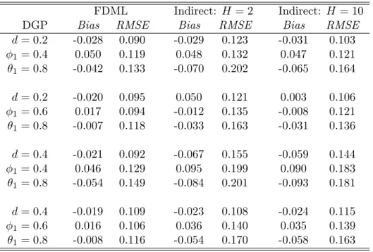
Two first order LMSV models are considered. The DGP for the LMSV(0, d,0) model is (28) and the DGP for the LMSV(1, d,1) model is (29). The indirect results for the LMSV(0, d,0) model are based on an AR(1) auxiliary model for the natural logarithm of the squared errors according to that in (40) while the indirect results for the LMSV(1, d,1) model are based on an AR(3) auxiliary model. The FDML estimator uses the likelihood function in (30) specified using (27). The DGP parameter values for each LMSV model are reported in Tables 4 and 5.
4.2 Comparison of Alternative Estimators: The FIGARCH Model
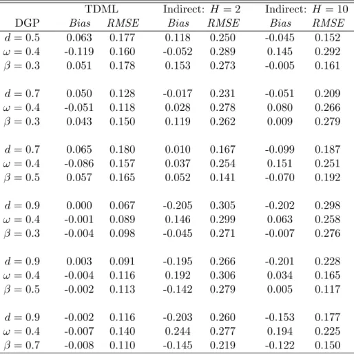
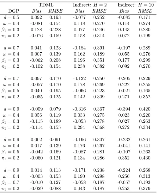
The bias and root mean square error (RMSE) of the TDML and indirect estimators for the FIGARCH DGP are reported in Tables 1 and 2. Across the two tables and the 12 DGP specifications, the bias levels for the estimators are mostly comparable; the TDML estimator is consistently the more efficient however. Despite this, the TDML estimator does struggle a few times, for example the bias levels for the d = 0.9, ω = 0.4, β1 = 0.3, π1 = 0.2 specification are high, but the indirect estimator appears to struggle more. The general performance of the indirect estimator seems to improve as H increases from 2 to 10. However, for the indirect estimator the results in these tables are not strong. The TDML estimator dominates in terms of bias and RMSE for nearly every specification. Further investigation into auxiliary models and simulation paths is necessary to establish the indirect estimator’s optimal properties.
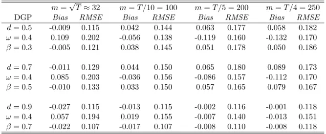
Table 3 reports the impact of the truncation parameter on the TDML estimator for the T = 1000 sample. Four truncation parameters are examined, ranging from m = √T ≈ 32 to m = T /4 ≈ 250, and three DGPs are utilized from Table 1. The results suggest the different truncation parameters used in the TDML estimator do not uniformly affect the finite sample properties of the estimator. It might be expected that asm increases bias may fall and RMSE rise, since the smaller estimation sample will reduce efficiency but avoid any starting value problems biasing the estimates. Table 3 suggests, at least for the sample size being considered, that the TDML estimator is reasonably robust to the values of
4.3 Comparison of Alternative Estimators: The LMSV Model
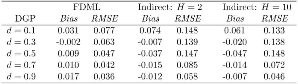
The small sample properties of the FDML and indirect estimators for the LMSV model are reported in Tables 4 and 5. Five values of dare considered for the LMSV(0, d,0) DGP in Table 4. The FDML estimator has superior finite sample properties; with RMSEs that are particularly low relative to the indirect estimator. The performance of the indirect estimator does appear to improve asH goes from 2 to 10. Table 5 suggests the performance of the indirect estimator improves relative to the FDML estimator for the slightly more complicated LMSV(1, d,1) DGP. Several of the RMSEs for the two estimators are reasonably close and the indirect estimator has a better bias estimate for a couple of the specifications; although this would not appear to be a strong result. Again, the performance of the indirect estimator improves as H goes from 2 to 10. Overall, it would appear the indirect estimator performs relatively better for the LMSV DGP than for the FIGARCH DGP.
5
Conclusion
The development, estimation and testing for long memory volatility models is a rapidly growing research area for econometricians and applied financial economists. Fractionally integrated models of conditional variance are important because of their empirical relevance and the flexibility they offer over the relatively rigid nature of integer restricted GARCH, IGARCH and SV models. Baille (1996) remarks that comparison of FIGARCH and LMSV models is a promising area for future research. However, as with fractionally integrated models for the conditional mean, the difficulties associated with estimation threaten to inhibit their widespread application. This paper has addressed this issue by extending the indirect estimator for ARFIMA models in Martin and Wilkins (1999) to fractionally integrated GARCH and fractionally integrated SV models. Simulation results comparing maximum likelihood and indirect estimators suggests there is scope for further investigation into alternative indirect estimator specifications.
References
[1] Baillie, R.T. (1996) Long memory processes and fractional integration in econometrics. Journal of Econometrics, 73, 5-59.
[2] Baillie, R.T., T. Bollerslev and H.O. Mikkelson (1996) Fractionally integrated generalized autore-gressive conditional heteroskedasticity.Journal of Econometrics, 74, 3-30.
[3] Bollerslev, T. (1986) Generalised autoregressive conditional heteroskedasticity. Journal of Econometrics, 31, 307-327.
[4] Bollerslev, T., R.Y. Chou and K.F. Kroner (1992) ARCH modelling in finance.Journal of Econo-metrics, 52, 5-59.
[5] Bollerslev, T. and R.F. Engle (1993) Common persistence in conditional variances. Economet-rica, 61(1), 167-186.
[6] Bollerslev, T., R.F. Engle and D.B. Nelson (1994) ARCH models. In R.F. Engle and D. McFadden,
The Handbook of Econometrics 4, North-Holland.
[7] Bollerslev, T. and H.O. Mikkelson (1996) Modeling and pricing long memory in stock market volatility.Journal of Econometrics, 73, 151-184.
[8] Bollerslev, T. and J.M. Wooldridge (1992) Quasi-maximum likelihood estimation and inference in dynamic models with time-varying conditional variances.Econometric Reviews, 11, 143-172.
[9] Breidt, F.J., N. Crato and P.J.F. de Lima (1998) The detection and estimation of long memory in stochastic volatility.Journal of Econometrics, 83, 325-348.
[10] Ding, Z. and C.W.J. Granger (1996) Modeling volatility persistence of speculative returns: A new approach.Journal of Econometrics, 73, 185-215.
[11] Ding, Z., C.W.J. Granger and R.F. Engle (1993) A long memory property of stock market returns and a new model.Journal of Empirical Finance, 1, 83-106.
[12] Engle, R.F. (1982) Autoregressive conditional heteroscedasticity with estimates of the variance of UK inflation.Econometrica, 50, 987-1008.
[13] Engle, R.F. and T. Bollerslev (1986) Modelling the persistence of conditional variances. Econo-metric Reviews, 5(1), 1-50.
[14] Fox, R. and M.S. Taqqu (1986) Large sample properties of parameter estimates for strongly de-pendent stationary Gaussian time series.Annals of Statistics, 14, 517-532.
[15] Gallant, R. and G. Tauchen (1996) Which moments to match? Econometric Theory, 12, 657-681.
[16] Geweke, J. and S. Porter-Hudak (1983) The estimation and application of long memory time series models.Journal of Time Series Analysis, 4, 221-238.
[17] Gourieroux, C.A., A. Monfort and E. Renault (1993) Indirect inference. Journal of Applied Econometrics, 8, s85-s118.
[18] Granger, C.W.J. and R. Joyeux (1980) An introduction to long-memory time series models and fractional differencing.Journal of Time Series Analysis, 1(1), 15-29.
[19] Harvey, A.C. (1993) Long memory in stochastic volatility. Working Paper. [20] Hosking, J. (1981) Fractional differencing.Biometrika, 68, 165-176.
[21] Martin, V.L. and N.P. Wilkins (1999) Indirect estimation of ARFIMA and VARFIMA models.
Journal of Econometrics, 93, 149-175.
[22] Nelson, D.B. (1991) Conditional heteroskedasticity in asset returns: A new approach. Economet-rica, 59, 347-370.
[23] Psaradakis, Z. and M. Sola (1995) Modelling long memory in stock market volatility: A fractionally
integrated generalised ARCH approach.Discussion Paper No. DP 12-95, London Business
School.
[24] Sowell, F. (1992a) Maximum likelihood estimation of stationary univariate fractionally integrated time series models.Journal of Econometrics, 53, 165-188.
[25] Sowell, F. (1992b) Modeling long-run behaviour with the fractional ARIMA model. Journal of Monetary Economics, 29, 277-302.
[26] Taylor, S. (1994) Modelling stochastic volatility: A review and comparative study.Mathematical Finance, 4, 183-204.
[27] Weiss, A.A. (1986) Asymptotic theory for ARCH models: Estimation and testing.Econometric Theory, 2, 107-131.
Table 1: Small Sample Properties of the FIGARCH(1, d,0) Estimators
TDML Indirect: H= 2 Indirect: H= 10
DGP Bias RMSE Bias RMSE Bias RMSE
d= 0.5 0.063 0.177 0.118 0.250 -0.045 0.152 ω = 0.4 -0.119 0.160 -0.052 0.289 0.145 0.292 β = 0.3 0.051 0.178 0.153 0.273 -0.005 0.161 d= 0.7 0.050 0.128 -0.017 0.231 -0.051 0.209 ω = 0.4 -0.051 0.118 0.028 0.278 0.080 0.266 β = 0.3 0.043 0.150 0.119 0.262 0.009 0.279 d= 0.7 0.065 0.180 0.010 0.167 -0.099 0.187 ω = 0.4 -0.086 0.157 0.037 0.254 0.151 0.251 β = 0.5 0.057 0.165 0.052 0.141 -0.070 0.192 d= 0.9 0.000 0.067 -0.205 0.305 -0.202 0.298 ω = 0.4 -0.001 0.089 0.146 0.299 0.063 0.258 β = 0.3 -0.004 0.098 -0.045 0.271 -0.007 0.276 d= 0.9 0.003 0.091 -0.195 0.266 -0.201 0.228 ω = 0.4 -0.004 0.116 0.192 0.306 0.034 0.165 β = 0.5 -0.002 0.113 -0.142 0.279 0.005 0.117 d= 0.9 -0.002 0.116 -0.203 0.260 -0.153 0.177 ω = 0.4 -0.007 0.140 0.244 0.277 0.194 0.225 β = 0.7 -0.008 0.110 -0.145 0.219 -0.122 0.150
Table 2: Small Sample Properties of the FIGARCH(1, d,1) Estimators
TDML Indirect: H= 2 Indirect: H = 10
DGP Bias RMSE Bias RMSE Bias RMSE
d= 0.5 0.092 0.193 -0.077 0.252 -0.085 0.171 ω = 0.4 -0.081 0.154 0.118 0.270 0.114 0.274 β1 = 0.3 0.128 0.228 0.077 0.246 0.143 0.280 π1 = 0.2 -0.076 0.159 0.158 0.314 0.072 0.199 d= 0.7 0.041 0.123 -0.184 0.391 -0.197 0.289 ω = 0.4 0.007 0.139 0.162 0.189 0.055 0.276 β1 = 0.3 -0.062 0.208 0.196 0.351 0.177 0.299 π1 = 0.2 -0.102 0.154 0.238 0.382 0.092 0.270 d= 0.7 0.097 0.170 -0.122 0.250 -0.205 0.229 ω = 0.4 -0.057 0.170 0.178 0.269 0.222 0.255 β1 = 0.5 0.040 0.195 -0.066 0.223 -0.021 0.165 π1 = 0.2 -0.055 0.125 0.142 0.309 0.271 0.352 d= 0.9 -0.009 0.079 -0.316 0.367 -0.394 0.420 ω = 0.4 0.056 0.119 0.033 0.275 0.023 0.220 β1 = 0.3 -0.115 0.189 -0.053 0.278 0.027 0.263 π1 = 0.2 -0.114 0.155 0.294 0.368 0.272 0.334 d= 0.9 0.002 0.091 -0.196 0.307 -0.232 0.261 ω = 0.4 0.017 0.139 0.176 0.267 -0.041 0.141 β1 = 0.5 -0.042 0.169 -0.087 0.281 -0.107 0.263 π1 = 0.2 -0.060 0.121 0.134 0.286 0.352 0.430 d= 0.9 0.014 0.113 -0.171 0.238 -0.224 0.268 ω = 0.4 -0.003 0.153 0.190 0.298 0.256 0.313 β1 = 0.7 -0.010 0.127 -0.058 0.187 -0.057 0.193 π1 = 0.2 -0.029 0.088 0.043 0.187 0.253 0.379
Table 3: Impact of Truncation on the TDML Estimator for the FIGARCH(1, d,0) DGP withT = 1000 Observations
m=√T ≈32 m=T /10 = 100 m=T /5 = 200 m=T /4 = 250
DGP Bias RMSE Bias RMSE Bias RMSE Bias RMSE
d= 0.5 -0.009 0.115 0.042 0.144 0.063 0.177 0.058 0.182 ω= 0.4 0.109 0.202 -0.056 0.138 -0.119 0.160 -0.132 0.170 β = 0.3 -0.005 0.121 0.038 0.145 0.051 0.178 0.050 0.186 d= 0.7 -0.011 0.129 0.044 0.150 0.065 0.180 0.089 0.173 ω= 0.4 0.085 0.203 -0.036 0.156 -0.086 0.157 -0.112 0.170 β = 0.5 -0.010 0.133 0.033 0.150 0.057 0.165 0.079 0.167 d= 0.9 -0.027 0.115 -0.013 0.115 -0.002 0.116 -0.001 0.118 ω= 0.4 0.057 0.194 0.019 0.155 -0.007 0.140 -0.013 0.151 β = 0.7 -0.022 0.107 -0.017 0.107 -0.008 0.110 -0.008 0.118
Table 4: Small Sample Properties of the LMSV(0, d,0) Estimators
FDML Indirect: H= 2 Indirect: H = 10
DGP Bias RMSE Bias RMSE Bias RMSE
d= 0.1 0.031 0.077 0.074 0.148 0.061 0.133
d= 0.3 -0.002 0.063 -0.007 0.139 -0.020 0.138
d= 0.5 0.009 0.047 -0.037 0.147 -0.047 0.148
d= 0.7 0.010 0.042 -0.015 0.085 -0.014 0.072
d= 0.9 0.017 0.036 -0.012 0.058 -0.007 0.046
Table 5: Small Sample Properties of the LMSV(1, d,1) Estimators
FDML Indirect: H= 2 Indirect: H= 10
DGP Bias RMSE Bias RMSE Bias RMSE
d= 0.2 -0.028 0.090 -0.029 0.123 -0.031 0.103 φ1 = 0.4 0.050 0.119 0.048 0.132 0.047 0.121 θ1 = 0.8 -0.042 0.133 -0.070 0.202 -0.065 0.164 d= 0.2 -0.020 0.095 0.050 0.121 0.003 0.106 φ1 = 0.6 0.017 0.094 -0.012 0.135 -0.008 0.121 θ1 = 0.8 -0.007 0.118 -0.033 0.163 -0.031 0.136 d= 0.4 -0.021 0.092 -0.067 0.155 -0.059 0.144 φ1 = 0.4 0.046 0.129 0.095 0.199 0.090 0.183 θ1 = 0.8 -0.054 0.149 -0.084 0.201 -0.093 0.181 d= 0.4 -0.019 0.109 -0.023 0.108 -0.024 0.115 φ1 = 0.6 0.016 0.106 0.036 0.140 0.035 0.139 θ1 = 0.8 -0.008 0.116 -0.054 0.170 -0.058 0.163