Discussion Papers are a series of manuscripts in their draft form. They are not intended for circulation or distribution except as indicated by the author. For that reason Discussion Papers may not be reproduced or distributed without the written consent of the author
CIRJE-F-184
Improving Small Sample Properties of the
Empirical Likelihood Estimation
Naoto Kunitomo University of Tokyo
Improving Small Sample Properties of the Empirical
Likelihood Estimation
∗Naoto Kunitomo†
November 2002
Abstract
We propose to use a simple modification of the maximum empirical likelihood (MEL) method for estimating structural equations in econometrics. The modified estimator improves both the asymptotic bias and the mean squared error of the MEL estimator in the orders ofO(n−1) andO(n−2),respectively, at the same time. It also improves the asymptotic bias of the generalized method of moments (GMM) estimation (or the estimating equation (EE) method) significantlywhen there are manyinstruments in the econometric literatures.
Key Words
Modified Empirical Likelihood Method, Estimating Structural Equation, Asymptotic Bias, Mean Squared Error, LIML Method, GMM Method
JEL Code: C-13, C-30
∗The author thanks Mr. Yukitoshi Matsushita for his assistance on preparing numerical examples
in Section 6 of the present work.
1. Introduction
The studyof estimating a single structural equation in econometric models has led to develop several estimation methods as the alternatives to the least squares esti-mation method. The classical examples in the econometric literatures are the limited information maximum likelihood (LIML) method and the instrumental variables (IV) method including the two-stage least squares (TSLS) method. See Anderson, Kunit-omo, and Sawa (1982) and Anderson, KunitKunit-omo, and Morimune (1986) for their finite sample properties, for instance. In addition to these classical methods the maximum empirical likelihood (MEL) method has been proposed and has gotten some attention recentlyin the statistical and econometric literatures. It is probablybecause the MEL method gives asymptotically efficient estimator in the semi-parametric sense and also improves the serious bias problem known in the estimating equation method or the generalized method of moments (GMM) method when the number of instruments is large in econometric models. See Owen (2001), Qin and Lawless (1994), and Kitamura, Tripathi, and Ahn (2001) on the details of the MEL method.
The main purpose of this studyis to propose a modification of the MEL estimation method for estimating a single structural equation and show that it improves the small sample properties of the MEL estimator. Our modification method is simple and it has an intuitive interpretation. Thus it is quite appealing from the views of theoryas well as practice. We shall show that the modified MEL estimator (which is abbreviated as the MMEL estimator) we are proposing in this paper has not onlythe smaller asymptotic bias in the order of O(n−1) but also the smaller asymptotic mean squared errors in the order of O(n−2) than the original MEL estimator at the same time where n is the sample size. Thus the MMEL estimation method we are proposing dominates the MEL estimation method in the asymptotic higher order sense. Also by investigating a set of simulations systematically we have found that the modified MEL estimator has better small sample properties in the sense of the bias, the mean squared error, and the probabilityconcentration than the MEL estimator in all cases.
In the econometric literatures the generalized method of moments (GMM) esti-mation method has been quite popular in the past decade. The GMM method was originallyproposed byHansen (1982) in the econometric literature and it is essentially the same as the estimating equation (EE) method proposed byGodambe (1960) which has been used in statistical applications. This approach has an attractive feature that it has rather broad applicabilityand it is easilyimplemented in statistical analyses. However, it has been known that there is a serious bias problem in the GMM estima-tion when there are manyinstruments in econometric models. In this respect we should notice that the MMEL estimator we are proposing is quite similar to the MEL estima-tor when there are manyinstruments. Hence the MMEL estimation method improves the MEL estimation while it retains the good small sample properties of the MEL es-timation method. In our limited simulations the MMEL estimator has better small sample properties in the sense of the bias, the mean squared error, and the probability concentration than the GMM estimator in all cases when the number of instruments is large. Therefore our new method is quite attractive for the problem of estimating econometric models in the semi-parametric sense.
(MEL) estimation method. In Section 3 we shall give a modified MEL estimation method for the problem of estimating a linear structural equation when there are in-strumental variables and the disturbances are homoscedastic. Then in Sections 4 and 5 we shall discuss the modified MEL estimation method for the heteroscedastic distur-bance case and the nonlinear structural equation case, respectively. In Section 6 we give some numerical examples and some conclusions are given in Section 7. The more detailed derivations of our results are given in the Appendix.
2. Estimating a Single Structural Equation by the Maximum Empirir-cal Likelihood Method
Let a single equation in the econometric model be given by
y1i =h(y2i,z1i, θ) +ui (i= 1,· · ·, n),
(2.1)
where h(·,·,·) is a function,y1i and y2i are 1×1 and G1×1 (vector of) endogenous
variables,z1i is aK1×1 vector of exogenous variables,θis an r×1 vector of unknown
parameters, and{ui}are mutuallyindependent disturbance terms withE(ui) = 0 (i=
1,· · ·, n).
We assume that (2.1) is the first equation in a system of (G1+ 1) structural equations relating the vector of G1 + 1 endogenous variables yi = (y1i,y2i) and the vector of
K (= K1+K2) exogenous variables {zi} which includes {z1i}. The set of exogenous
variables{zi}are often called the instrumental variables and we have the orthogonality
condition
E(uizi) =0 (i= 1,· · ·, n).
(2.2)
Because we do not specifythe equations except (2.1) and we onlyhave the limited information on the set of instrumental variables or instruments, we onlyconsider the limited information estimation methods. When the function h(·,·,·) is of the linear form, (2.1) can be written as
y1i = (y 2i,z 1i)( β γ ) +ui (i= 1,· · ·, n), (2.3)
whereθ = (β, γ) is a 1×p(p=K1+G1) vector of unknown coefficients.
Furthermore, when all structural equations in the econometric model are linear, the reduced form equations ofyi = (y1i,y
2i) can be defined by yi =Π zi+vi (i= 1,· · ·, n), (2.4) wherevi= (v1i,v
2i) is a 1×(1 +G1) disturbance terms withE[vi] =0
and Π = ( π 1 Π2 ) (2.5)
is a (1 +G1)×K partitioned matrix of the linear reduced form coefficients. Bymulti-plying (1,−β) from the left-hand side, we have the restriction
(1,−β)Π = (γ,0) .
The maximum empirical likelihood (MEL) estimator for the vector of unknown parametersθ in (2.1) is defined bymaximizing the Langrangian form
L∗n(λ, θ) = n i=1 logpi−µ( n i=1 pi−1)−nλ n i=1 pizi[y1i−h(y2i,z1i, θ)], (2.7)
whereµ and λ are a scalor and aK×1 vector of Lagrangian multipliers, andpi (i=
1,· · ·, n) are the weighted probabilityfunctions to be chosen. It has been known (see Qin and Lawles (1994) or Owen (2001)) that the above maximization problem is the same as to maximize Ln(λ, θ) =− n i=1 log{1 +λzi[y1i−h(y2i,z1i, θ)]}, (2.8)
where we have the conditions ˆµ=n ,and [npˆi]−1= 1 +λ
zi[y1i−h(y2i,z1i, θ)].
(2.9)
Bydifferentiating (2.7) with respect to λ and combining the resulting equation with (2.9), we have the relation
n i=1 ˆ pizi [y1i−h(y2i,z1i, θ)] =0 (2.10) and ˆ λ= [ n i=1 ˆ piu2i( ˆθ)ziz i]−1[ 1 n n i=1 ui( ˆθ)zi], (2.11)
where ui( ˆθ) = y1i −h(y2i,z1i,θˆ) and ˆθ is the maximum empirical likelihood (MEL)
estimator for the vector of unknown parameters θ . From (2.7) the MEL estimator of
{θ} is the solution of the set ofp equations ˆ λ n i=1 ˆ pizi[− ∂h(y2i,z1i,θˆ) ∂θj ] = 0 (j = 1,· · ·, p). (2.12)
When the structural equation of (2.1) is linear, the MEL estimator of the vector of coefficient parametersθ = (β, γ) can be simplified as the solution of
[ n i=1 ˆ pi( y2i z1i )zi][ n i=1 ˆ piui( ˆθ)2ziz i]−1[ 1 n n i=1 zi y1i] (2.13) = [ n i=1 ˆ pi( y2i z1i )zi][ n i=1 ˆ piui( ˆθ)2ziz i]−1[ 1 n n i=1 zi(y 2i,z 1i)]( ˆ β ˆ γ ).
If we substitute 1/nfor ˆpi (i= 1,· · ·, n) in (2.13), then we have the generalized method
of moments (GMM) estimator for the vector of coefficient parameters θ = (β, γ),
which is the solution of [1 n n i=1 ( y2i z1i )zi][ 1 n n i=1 ui( ˆθ)2ziz i]−1[ 1 n n i=1 ziy1i] (2.14) = [1 n n i=1 ( y2i z1i )zi][ 1 n n i=1 ui( ˆθ)2ziz i]−1[ 1 n n i=1 zi(y 2i,z 1i)]( ˆ β ˆ γ ),
where ˆθis an initial (consistent) estimator of θ .( See Hayashi (2000) on the details of the GMM method in econometrics, for instance. )
3. A Modified MEL Estimation in the Linear Homoscedastic Case
The most important feature of the MEL estimation is the use of the estimated weight functions ˆpi (i= 1,· · ·, n).We notice that if we substitute (1/n) for ˆpi (i= 1,· · ·, n),
the resulting estimation method is identical to the estimating equations method or the generalized method of moments (GMM) in the econometric literatures. This is a simple fact which lead us to consider a simple modification of the MEL method we are proposing in this paper.
Let ˆ p∗i = 1 n[1 +δ λziui( ˆθ)] , (3.1)
where δ is a positive constant (0 ≤ δ ≤ 1) and ˆθ is the MEL estimator of θ . Then we can define a modification of the MEL estimation bysubstituting ˆpi (i = 1,· · ·, n)
into (2.9)-(2.11). We shall denote the resulting Lagrangian multiplier and the modified estimator as ˆλ∗ and ˆθ∗ .
In the rest of the present paper we shall consider the standardized error of estimators as ˆ e=√n( βˆ−β ˆ γ−γ ) , (3.2)
where ˆθ = ( ˆβ,γˆ) . We denote ˆefor the MEL estimator and its modification as ˆeEL
and ˆe∗,respectively.
In this section we consider the situation that the disturbances are homoscedas-tic random variables. Under a set of regularityconditions, the asymptohomoscedas-tic variance-covariance matrix of the asymptotically efficient estimators in the semi-parametric framework is given by Q−1 =DMC−1MD, (3.3) whereC=σ2Mand D = [Π2,( IK1 O )], (3.4) M = plimn→∞1 n n i=1 ziz i . (3.5)
Here we have implicitlyassumed that E(u2i) = σ2 (>0), the (constant) matrix M is positive definite, and the rank condition
rank(D) =p(=G1+K1).
(3.6)
These conditions assure that the limiting variance-covariance matrixQis non-degenerate. The rank condition implies the order condition
L=K−p≥0,
(3.7)
In order to compare alternative efficient estimation methods in the asymptotic sense, we need to derive the asymptotic expansions of the density functions of the standardized estimators (3.2) in the form of
f(ξ) =φQ(ξ)[ 1 +√1 nH1(ξ) + 1 nH2(ξ) ] +o( 1 n), (3.8) whereξ = (ξ1,· · ·, ξp)
, φQ(ξ) is the multivariate normal densityfunction with mean
0 and the variance-covariance matrix Q , and Hi(ξ) (i = 1,2) are some polynomial
functions of elements of ξ. For the rest of our arguments we need a set of regularity conditions.
Assumption I:
(i) The sequence of random vectors {ui ,v
i} are independentlyand
identicallydis-tributed, and their sixth order moments are bounded. (ii) We have the rank condition given by(3.6).
(iii) The sequence of exogenous variables{zi} are random vectors or non-random (i.e.
deterministic) vectors, but theyare i.i.d. random variables being independent of{ui},
and their sixth order moments are bounded in the first case. Theysatisfy(iii-a) 1
n1max≤i≤n|zi|
2 p
−→0 (3.9)
asn−→ ∞,(iii-b) there exists (constant) positive definite matrixM such that 1 n n i=1 ziz i (=Mn) =M+Op( 1 √ n), (3.10)
and (iii-c) we have the condition 1 n n i=1 E[z(ij)zi(k)zi(l)u3i] =O(√1 n) , (3.11)
where we denote theK×1 vector zi = (z( j) i ).
When {zi} are a sequence of i.i.d. random vectors, we have the notation C =
E[u2iziz
i] =σ2E(ziz
i) (i= 1,· · ·, n).
We notice that the conditions inAssumption Iare rather strong, but the conditions lead to some simplifications in the derivations and the resulting expressions of the asymptotic bias (ABIAS) and the asymptotic meas suared errors (MSE). Nonetheless, these conditions can be relaxed considerablyat the cost of complicated derivations and notations. Some possible directions will be given in the next two sections. We expect that the most of the results we are reporting in this paper are essentiallytrue under a set of the weaker conditions.
We shall use the mean operator AMn(ˆe), which is defined as the mean of ˆe with
respect to the asymptotic expansion of its density function of the standardized estima-tors up toO(n−1).Then we write the asymptotic bias and the asymptotic MSE of the standardized estimator by ABIASn(ˆe) =AMn(ˆe),and
AM SEn(ˆe) =AMn(ˆeeˆ
).
Furthermore, as an important criterion we shall use the asymptotic probability of con-centration (APC)
AP Cn=P( ˆe∈S),
where the integrand is taken with respect to the asymptotic expansion of the density function of estimators up toO(n−1) in the form of (3.8) andS is anystar-shaped set. ( Here we define that for anyreal number α ∈ [0,1] αS ∈ S if S is a star-shaped. ) This criterion is important in the present case because there are important cases when the estimators do not posses moments. For instance, it has been known that the LIML estimator does not have anyinteger order moments. (see Anderson et. al. (1982)). For the asymptotic bias of the modified MEL estimator, we have the following result and its derivation is given in the Appendix.
Theorem 3.1 : Under Assumption I, the asymptotic bias (ABISAS) of ˆe∗ as n →
+∞ is given by AMn(ˆe∗) = 1 √ nQ q[L−1−δL], (3.12)
where q is thep×1 vector given by
q= 1
σ2Cov((
v2i
0 )ui) (i= 1,· · ·, n).
(3.13)
Byusing this result we immediatelyobserve that the asymptotic bias of the MEL estimator and the GMM estimator are (−1)Q q/√nand (L−1)Q q/√n,respectively. Then it is possible to remove the asymptotic bias of the MEL estimator by setting
δ∗= L−1
L
provided that L > 0 . One interpretation of this modification is that δ∗ is a kind of shrinkage factor to the estimated Lagrangian multiplierλand hence the estimators of probabilityparameters{pi}. We now state the main result whose proof is given in the
Appendix.
Theorem 3.2 : Suppose we chooseδ∗L=L−1 (L≥1)in the class of modified MEL estimators. Then under Assumption I,
lim n→∞n[AM SEn(ˆe ∗)−AM SE n(ˆeEL)]≤0 (3.14) and lim n→∞n[AP Cn(ˆe ∗)−AP C n(ˆeEL)]≥0 (3.15)
asn→ ∞.The strict inequalities in (3.14) and (3.15) hold whenq=0 in the positive definite sense, where qis given by (3.13).
4. The Linear Heteroscedastic Case
The results reported in Section 3 can be extended to the case when the disturbances are heteroscedasticallydistributed under a set of additional assumptions. The limiting
variance-covariance matrix of the standardized errors for the estimator ˆein this case shoud be modified as Q−1 =DMC−1MD, (4.1) where C= lim1 n n i=1 E[u2iziz i], (4.2)
provided that the (constant) matrix M is positive definite, the probabilitylimit (con-stant) matrix C is positive definite, and sup1≤i≤nE(u2i) < +∞ . For deriving the asymptotic bias (ABIAS) and the asymptotic mean squared errors (AMSE), we need stronger regularityconditions.
Assumption II:
(i) The sequence of random vectors {ui,v
i} are a sequence of martingale differences
with E[(ui,v
i)|Fi−1] = 0
(i= 1,· · ·, n) and their sixth order moments are bounded, where Fi−1 is theσ−field generalted by(uj,vj) (j ≤ i−1) and zj (j≤i) .( We use
the convention thatF0 contains onlythe null set. ) Also there exists ap×1 constant vectorqsuch that wi = (v
2i,0 )−qui and q= 1 σ2iCov(( v2i 0 )ui) +o( 1 √ n), (4.3) whereE(u2i) =σi2 (i= 1,· · ·, n).
(ii) We have the rank condition given by(3.6).
(iii) The sequence of exogenous variables{zi} are random vectors or non-random (i.e.
deterministic) vectors, but theyare stationary, ergodic and their sixth order moments are bounded in the former case. Also theysatisfythe conditions (3.9)-(3.11) in As-sumption Iand there exists a (constant) positive definite matrixCsuch that
1 n n i=1 u2i ziz i =C+Op( 1 √ n). (4.4)
We notice that while some conditions are automaticallysatisfied for the heteroscedas-tic normal disturbances, theycan be restrictive. In order to remove the asymptoheteroscedas-tic bias of the MEL estimator in the more general case, however, we need to have more compli-cated modifications. In this paper we restrict our discussions to the simple modification method which can be practical for real applications. If we have the situation
plim1 n n i=1 E(u2i) =σ2 (>0) (4.5)
and the variables {zi} are a sequence of i.i.d. random vectors, and ziz
i are
asymp-toticallyuncorrelated with u2i ,then we have C=σ2M and the asymptotic variance-covariance matrix reduces to (3.3). For the asymptotic bias of the modified MEL estimator, we have the following result.
Theorem 4.1 : Under Assumption II, the asymptotic mean function of eˆ∗ as n →
+∞ is given by AMn(ˆe∗) = 1 √ nQ q[L−1−δL] . (4.6)
Byusing this result on the asymptotic bias of the general modified MEL estimator, we have the next result on the asymptotic MSE and the asymptotic PC as Theorem 3.2.
Theorem 4.2 : Suppose we chooseδ∗L=L−1 (L≥1)in the class of modified MEL estimators. Then under Assumption II,
lim n→∞n[AM SEn(ˆe ∗)−AM SE n(ˆeEL)]≤0 (4.7) and lim n→∞n[AP Cn(ˆe ∗)−AP C n(ˆeEL)]≥0 (4.8)
as n → ∞ . The strict inequalities in (4.7) and (4.8) hold if q = 0 in the sense of positive definiteness and q is defined by (4.3).
5. The Nonlinear Case
When the structural equation in (2.1) is nonlinear, we have similar arguments and our modification of the MEL estimation method can be still useful. However, we need complicated notations and a set of additional regularityconditions including the differentiabilities of the function h(·,·,·) . For the nonlinear function h(·,·,·),we use the notation gi(θ) =zi [y1i−h(y2i,z1i, θ)] (i= 1,· · ·, n) (5.1) and let C = plim[1 n n i=1 gi(θ0)g i(θ0)], (5.2) D(M) = plim1 n[− n i=1 ∂gi(θ0)], (5.3)
where θ0 = (θ0(i)) is a p×1 vector of true value of the unknown parameters θ and
∂gi(θ) = (∂g∂θi(iθ)).
We assume aK×K matrixCis positive definite and aK×p matrixD(M) is of full rank ( p ≤ K ). Then the asymptotic variance-covariance matrix of asymptotically efficient estimators in the semi-parametric sense can be given by
Q= [D(M)C−1D(M)]−1 ,
(5.4)
provided that it is non-singular.
In order to derive the asymptotic bias of the MEL estimator, we consider the situation when we have the nonlinear relations
y2i = Π2(zi,v2i, π2),
(5.5)
∂hi
∂θ = qui+m(wi,zi, θ),
(5.6)
whereπ2 = (π2ij) is a vector of unknown parameters, v2i is a vector of random terms, wi=m(wi,zi, θ)−E[m(wi,zi, θ)] (i= 1,· · ·, n),
p×1 random vectors which are uncorrelated withui and E[wi] =0. Assumption III:
(i) The same conditions as (i) in Assumption II. (ii) The K×pmatrix D(M) is of full rank and it is p.
(iii) We assume the same conditions on{zi}as (iii) ofAssumption II. Also the functions
gi(θ) are twice continuouslydifferentiable and their sixth order moments are bounded.
There exist constant matricess Cand D(M) such that 1 n n i=1 gi(θ)g i(θ) = C+Op( 1 √ n), (5.8) (−1)1 n n i=1 ∂gi(θ) = D(M) +Op( 1 √ n). (5.9)
(iv) The true value θ0 of unknown parameters is an interior point of the compact parameter space Θ.
We note that the conditions in Assumption IIIare pararell to those inAssumption IandAssumption II in the linear case. In the simplest linear homoscedastic case when
{zi} are a sequence of i.i.d. random vectors, then D(M) =MDand C=σ2M.
For the asymptotic bias of the modified MEL estimator, we have the following result and its proof is given in the Appendix.
Theorem 5.1 : Under Assumption III, the asymptotic bias of the standardized esti-mator ˆe∗ as n→+∞ is given by AMn(ˆe∗) = 1 √ nQ q[L−1−δL]− 1 √ n[( 1 2)Q D(M) C−1tr(FQ)], (5.10) where F= (fjk) and fjk = plim 1 n n i=1 zi ∂2hi ∂θj∂θk .
Byusing this result we immediatelyobserve that the asymptotic bias of the MEL estimator and the GMM estimator have the corresponding terms as in the linear case and there is a common extra term due to the nonlinear relation in (2.1). Then it is possible to reduce the asymptotic bias of the MEL estimator by using the same modification of the MEL estimation method given that the second bias term in (5.10) is not verylarge. This is the case when the degrees of overidentification L is large.
The asymptotic expansions of the density functions of the modified MEL estima-tor and its asymptotic mean squared error have many terms in the general nonlinear case. However, we expect that the similar results asTheorem 3.2 would hold in many situations under a set of additional regularityconditions.
6. Some Simulations
In order to investigate the finite sample properties of the MEL estimation method and our modified MEL estimation method, we have done a set of numerical simulations. For this purpose we set a simple linear structural model
y1i =β1+β2y2i+γ1z1i+ui ,
where yki (k = 1,2) are the endogenous variables, z1i is an exogenous variable, and
βi (i= 1,2) and γ1 are constant coefficients. We have investigated the situation when
the endogenous variable y2i can be solved as
y2i =π20+π21z1i+π
22z2i+v2i ,
(6.2)
whereπ2j (j= 0,1) are scalor coefficients, π22is aK2×1 vector of coefficients, andz2i
is a vector of instrumental variables. BecauseG1= 1,the degrees of overidentification
L=K2−1 in the present case. We first setL= 3,5,10,20;n= 50,100,and then we simulated the normal random numbers for the exogenous variables zi = (z1i,z
2i), the
disturbance terms ui , and the endogenous variables (y1i, y2i) (i = 1,· · ·, n) byusing
the Gaussian number generators. The number of replications in each case is 5,000. We have summarized our simulation results in Table 6. For the sake of comparison we have given the mean squared error (MSE), the mean absolute error (MAE), and the probabilityof concentration (PC) for the GMM estimator, the MEL estimator, and the Modified MEL (MMEL) estimator. The PC has been calculated as
P C =P(|√nQ11−1/2( ˆβ−β)| ≤c),
(6.3)
where ˆβ is the estimator ofβ andQ11is the (1,1) element ofQwhich is the asymptotic variance-covariance matrix of the standardized estimator ˆe.We have used the normal-ization or standardnormal-ization because it is often easyto make comparisons of alternative estimation methods and we setc= 1 for our numerical analysis.
Table 6.1 :Finite Sample Properties of Estimators (L=5, n=50)
Bias MSE MAE PC GMM -0.0567 0.8367 0.7479 0.6018
MEL 0.0180 1.0930 0.7700 0.6418 MMEL 0.0005 0.9107 0.7345 0.6422
Table 6.2 :Finite Sample Properties of Estimators (L=10, n=50)
Bias MSE MAE PC GMM -0.0671 0.6146 0.6526 0.5100
MEL 0.0093 0.6911 0.6373 0.5672 MMEL 0.0003 0.6361 0.6189 0.5734
Table 6.3 :Finite Sample Properties of Estimators (L=3, n=100)
Bias MSE MAE PC GMM -0.0207 0.5475 0.5905 0.6552
MEL 0.0115 0.6164 0.6068 0.6662 MMEL -0.0002 0.5684 0.5898 0.6724
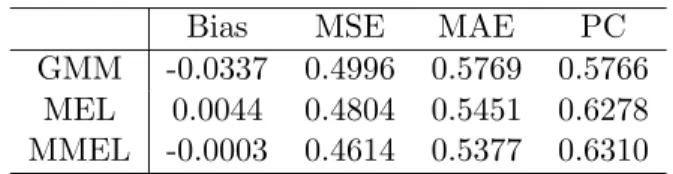
Table 6.4 :Finite Sample Properties of Estimators (L=10, n=100)
Bias MSE MAE PC GMM -0.0337 0.4996 0.5769 0.5766
MEL 0.0044 0.4804 0.5451 0.6278 MMEL -0.0003 0.4614 0.5377 0.6310
Table 6.5 :Finite Sample Properties of Estimators (L=15, n=100)
Bias MSE MAE PC GMM -0.0358 0.3369 0.4759 0.5118
MEL 0.0037 0.3148 0.4392 0.5810 MMEL 0.0013 0.3046 0.4337 0.5892
There are several interesting findings on the small sample properties of the alterna-tive estimation methods from the set of our experiments.
First, in terms of the MSE and MAE criteria the GMM estimator often performs well when L is small. In such cases the MEL estimator perform well in term of the probabilityof concentration. Thus we should be careful on the choice of loss functions when we want to compare alternative estimation methods in order to make a fair comparison of alternative estimation methods. ( See Anderson et. al. (1982) on the related issues. ) Second, the good performance of the GMM estimator becomes deteriolated quicklyas the number of instruments L becomes large. This is the case regardless of the choice of criteria for comparison. On the other hand, the MEL method outperforms the GMM estimator in this situation byusing anycriteria.
Most importantly, in all cases the modifoed MEL (MMEL) estimator outperforms the MEL estimator in the sense of the Bias, the MSE, the MAE, and the PC. When L is large, the MMEL estimator is better than the MEL estimator, but the differences are not large.
On the whole these findings agree with our investigations on the finite sample prop-erties based on the asymptotic expansions of the density functions of estimators up to
O(n−2) in the previous sections. It is consistent with the studyon the small sample properties of the MEL estimator and the GMM estimator byKunitomo and Matsushita (2002). Theyhave given extensive tables of the distribution functions of two estimators in the linear homoscedastic case.
7. Conclusions
We have proposed a new estimation method of a structural equation bymodifying the maximum empirical likelihood (MEL) method. Our estimator (MMEL) has not onlythe smaller asymptotic bias than the MEL estimator but also has the smaller asymptotic mean squared error when the sample size is large. Also we have given the numerical examples which suggest that the new estimation method has better small sample properties than the original MEL estimation method. Therefore we should use the modified MEL estimation method whenever we want to use the MEL estimation method for practical purposes. Also our modified estimator has good small sample properties when the degree of overidentification is large. It has been known that the GMM estimator has large bias in such situations and our method gives an alternative estimation method in this respect.
We should mention that the empirical likelihood (EL) method has been originally developped as the non-parametric testing and constructing confidence interval prob-lems. (See Owen (2001) in the details.) In this respect there would be some useful ways to incorporate the modified MEL estimation method proposed in this paper for the related problems. It is currentlyunder investigation.
References
[1] Anderson, T.W., N. Kunitomo, and T. Sawa (1982), “Evaluation of the Distribu-tion FuncDistribu-tion of the Limited InformaDistribu-tion Maximum Likelihood Estimator,” Econo-metrica, Vol. 50-4, 1009-1027.
[2] Anderson, T.W., N. Kunitomo, and K. Morimune (1986), “Comparing Single Equation Estimators in a Simultaneous Equation System,” Econometric Theory, Vol. 2, 1-32.
[3] Fujikoshi, Y., K. Morimune, N. Kunitomo, and M. Taniguchi (1982), “Asymptotic Expansions of the Distributions of the Estimates of Coefficients in a Simultaneous Equation System,” Journal of Econometrics, Vol. 18, 2, 191-205.
[4] Godambe, V.P. (1960), “An Optimum Propertyof Regular Maximum Likelihood Equation,” Annals of Mathematical Statistics, Vol. 31, 1208-1211.
[5] Hansen, L. (1982), “Large Sample Properties of Generalized Method of Moments Estimators,” Econometrica, Vol. 50, 1029-1054.
[6] Hayashi, F. (2000),Econometrics, Princeton UniversityPress.
[7] Kitamura, Y. G. Tripathi, and H. Ahn (2001), “Empirical Likelihood-Based Infer-ence in Conditional Moment Restriction Models,” Unpublished Manuscript. [8] Kunitomo, N. and Y. Matsushita (2002), “On Finite Sample Distributions of
the Empirical Likelihood Estimator and the GMM Estimator,” Unpublished Manuscript (in preparation).
[9] Morimune, K. (1985), Estimation and Testing of Econometric Models, Kyoritsu (in Japanese).
[10] Newey, W. K. and R. Smith (2001), “Higher Order Properties of GMM and Gen-eralized Empirical Likelihood Estimator,” Unpublished Manuscript.
[11] Owen, A. B. (1990), “Empirical Likelihood Ratio Confidence Regions,”The Annals of Statistics, Vol. 22, 300-325.
[12] Owen, A. B. (2001),Empirical Likelihood, Chapman and Hall.
[13] Qin, J. and Lawless, J. (1994), “Empirical Likelihood and General Estimating Equations,” The Annals of Statistics, Vol. 22, 300-325.
Mathematical Appendix
In this appendix, we give the mathematical details of derivations omitted in the previous sections. There are two cases depending on whether the sequence of exogenous variables
{zi}are random vectors or non-random (i.e. deterministic) vectors. In order to simplify
our proofs and to avoid tedious derivations, we shall discuss the non-random case under the additional conditon Mn=M+O(n1).Nonetheless, other cases can be handled in
the similar ways as we shall discuss in this Appendix.
Appendix A : Derivations of Asymptotic Expansions
[A-1]: First we applythe similar arguments used in Owen (1990) and Qin and Lawless (1994) on the probabilitylimits and the consistencyof the MEL estimator. Then we have npˆi
p
→ 1, θˆEL p
→ θ0, (θ0 is the true value of θ) and √nˆλconverges to a random vector asn→ ∞.
In the linear case we substitute (2.1) into (2.13) and we have the corresponding representation of the standardized estimator ˆeas
[ n i=1 ˆ pi( y2i z1i )zi][ n i=1 ˆ piui( ˆθ)2ziz i]−1[ 1 √ n n i=1 ziui] (A.1) = [ n i=1 ˆ pi( y2i z1i )zi][ n i=1 ˆ piui( ˆθ)2ziz i]−1[ 1 n n i=1 zi(y 2i,z 1i)]ˆe,
where we use the notation ˆθ for ˆθEL without anysubscript whenever we do not have
anyconfusion. Asn→ ∞,we write the first order term of ˆeas ˜e0,which is given by ˜ e0 = [D(plimn1 n i=1 ziz i)(plim 1 n n i=1 ziz iu2i( ˆθ))−1(plim 1 n n i=1 ziz i)D]−1 (A.2) ×[D(plim1 n n i=1 ziz i)(plim 1 n n i=1 ziz iu2i( ˆθ))−1( 1 √ n n i=1 ziui).
The probabilitylimits and the random variable on the right hand side of (A.1) have been defined properlybecause the matricesMand Care non-singular andD is of full rank byour assumptions. Byusing the central limit theorem (CLT) to the last term, we have the weak convergence
˜
e0−→d Np(0,Q),
(A.3)
where a p×p matrix Q has been defined by(3.3) and −→d means the convergence of distribution asn→ ∞.Also asn→ ∞we notice that
1 √ n n i=1 ziui( ˆθ) = 1 √ n n i=1 ziui+ 1 n[− n i=1 zi(y 2i,z 1i)ˆe] (A.4) = √1 n n i=1 ziui−( 1 n n i=1 zizi)Deˆ+Op( 1 √ n).
Then byutilizing the representation of (2.11) for ˆλ ,we have √ nλ−λ0 −→p 0, (A.5) where λ0 =C−n1/2[IK−C−n1/2MnD(D MnC−n1MnD)−1D MnC−n1/2][C−n1/2 1 √ n n i=1 ziui],
and we have denotedK×K matricesMn= 1n
n i=1ziz i andCn= n1 n i=1u2iziz i .The random variable Bn=C−1/2 1 √ n n i=1 ziui (A.6)
converges to NK(0,IK) byCLT, and Mn p
−→ M, Cn p
−→ C as n −→ +∞ under
Assumption I, whereCis defined by(4.2). Hence we also have the convergence
C1n/2
√
nλˆ−→d NK(0,P¯E),
(A.7)
and the projection matrix onE is defined by ¯
PE =IK−E(E
E)−1E ,
(A.8)
which is constructed byaK×pmatrix E=C−1/2MD and E
n =C−n1/2MnD p
−→E
asn−→+∞.
[A-2]: The method we shall use to derive the asymptotic expansion of the density function of the standardized estimator ˆe is similar to the one used in Fujikoshi et. al. (1982) and Anderson et. al. (1986). The validityof the asymptotic expansions can be given bylengthyarguments which are similar to Appendix C of Fujikoshi et. at. (1982). We first derive the asymptotic expansion of the density function of the standardized estimator when the disturbance terms are normallydistributed. Then we shall consider the same problem for more general disturbances.
Byexpanding (3.2) and (2.13) with respect to ˜e0,formallywe can write
ˆ e= ˜e0+ [e0−˜e0] +√1 ne1+ 1 ne2+op( 1 n), (A.9) and √ nˆλ=λ0+√1 nλ1+ 1 nλ2+op( 1 n), (A.10) where we denote e0 = [DMnCn−1MnD]−1[D MnC−n1 1 √ n n i=1 ziui]. (A.11)
Bysubstituting these expansions into (2.9), we can also expand the estimated proba-bilityfunction as npˆi = 1 + 1 √ np (1) i + 1 np (2) i +op( 1 n), (A.12)
where p(1)i = −λ0zi[ui− 1 √ nz iDe0] p(2)i = −λ1zi[ui− 1 √ n(y 2i,z 1i)e0] +λ0zi[ 1 √ n(y 2i,z 1i)e1+ (v 2i,0 )e0] + (λ0zi)2[ui− 1 √ n(y 2i,z 1i)]2.
Byusing the relation
(y2i,z 1i) =z iD+w i+q ui, (A.13) we shall expand ˆ Cn = n i=1 ˆ piu2i( ˆθ)ziz i (A.14) = Cn+ 1 √ nCˆ (1) n + 1 nCˆ (2) n +op( 1 n) = Cn+ 1 √ nC (1) n + 1 nC (2) n +op( 1 n), and n i=1 ˆ pi( y2i z1i )zi = [D Mn] + 1 √ nE (1) n + 1 nE (2) n +op( 1 n), (A.15)
where we denote the random matrices as ˆ C(nj) = 1 n n i=1 p(ij)ziz iu2i( ˆθ) (j = 1,2), (A.16) E(1)n = 1 √ n n i=1 ( v2i 0 )z i+D 1 n n i=1 p(1)i ziz i+ 1 n n i=1 p(1)i ( v2i 0 )z i , (A.17) E(2)n = D 1 n n i=1 p(2)i ziz i+ 1 n n i=1 p(2)i ( v2i 0 )z i. (A.18)
Byusing (A.12)-(A.14), we notice thatC(1)n can be rewritten as C(1)n = 1 n n i=1 ziz i[p(1)i u2i + 2ui(−1)(y 2i,z 1i)e0] = 1 n n i=1 ziz i[−2(q e0)u2i −2ui(w i+z iD)e0−λ ziu3i] +Op( 1 √ n) = (−2)(qe0)Cn+ [−2 1 n n i=1 ziz iui(w i+z iD)e0− 1 n n i=1 ziz iu3iλ0] +Op( 1 √ n).
Bysubstituting the above expressions into (A.1) for ˆe,ˆλ,and ˆpi (i= 1,· · ·, n),we can
determine each terms of the stochastic expansions in the recursive wayas
e1 = −QnD MnC−n1[ 1 √ n n i=1 zi(v 2i,0)]e0 (A.19) +Qn[A1][ 1 √ n n i=1 ziui−MnD e0], e2 = Qn[A2][ 1 √ n n i=1 ziui−MnD e0] (A.20) −Qn[A1][MnDe1+ 1 √ n n i=1 zi(v 2i,0 )e0] −QnD MnC−n1 1 √ n n i=1 (v2i,0 )e1 ,
where we have used the corresponding notations
Q−n1 =D MnC−n1MnD, A1 =−DMnC−n1Cn(1)C−n1+E(1)n C−n1 , A2 =DMn[−C−n1C(2)n C−n1+C−n1Cn(1)C−n1C(1)n C−n1]−E(1)n C−n1C(1)n C−n1 +E(2)n C−n1 .
We also define two random vectors ˜e1 and ˜e2 bysubstitutingC forCn in (A.19) and
(A.20), respectively. Our next strategy is to derive the asymptotic expansion of the densityfunction of the random vector
˜
e= ˜e0+√1ne˜1+n1˜e2+op(
1
n)
(A.21)
and then we shall evaluate the effects of the differences in the form [ˆe−˜e] = [e0−˜e0] +√1n[e1−˜e1] + n1[e2−˜e2] +op(
1
n).
(A.22)
Although there are manyterms in the above stochastic expansion of ˜e,manyof them can be ignored for order calculations. This consideration leads to some simplifications of its stochastic expansions.
Because (1 n) n i=1 ˆ p(1)i ziz i= (−1) 1 n n i=1 ziz iλ ziui=Op( 1 √ n),
and we have the relation that
E(1)n ∼= 1 √ n n i=1 wiz i+q[ 1 √ n n i=1 uiz i−δλ 0Cn] +Op( 1 √ n), (A.23)
we have the effect of our modification of the MEL estmation onlyin the last term for the asymptotic bias. By using the relation
−QDMC−1[√1 n n i=1 ziui](q e0)∼=−˜e0(q˜e0) +Op( 1 √ n),
we can calculate the conditional expectation of each terms ine1 given x,which is the limiting random vector of e0,under the assumption of normal disturbances. Since the
random vectors ˆe and √nλ converge to the normal random variables, the effects of nonnormalityoccur in higher orders which should be evaluated later. The conditional asymptotic bias is given as
E[˜e1|x] =−(qx)x+Q q[L−δL] +Op(
1
√ n),
(A.24)
where we have used the relation on the projection operators such as PEP¯E = O ( PE =E(E
E)−1E is aK×K projection matrix ) and
λ0C1n/2P¯EBn=B nP¯EBn d −→χ2(L) (A.25)
as n → ∞ . We notice that e0 and BnP¯EBn are independent under the assumption
of normal disturbances. ( In fact theyare asymptoticallyindependent in the general case. ) We also have
e0 e0=QnD MnC−n1( 1 √ n n i=1 uizi 1 √ n n i=1 uiz i)C−n1MnDQn p −→Q
as n → ∞ and Q is non-singular. Then we have the results on the asymptotic bias for the class of modified MEL estimators inTheorem 3.1 and Theorem 4.1. It is easily seen that the formula for the asymptotic bias does not depend on the distribution of disturbances.
[A-3]: Since there are manyterms in the expression of e2 and ˜e2, at first it looks
formidable to evaluate the stochastic orders of these terms. Fortunately, we can show that we can ignore manyterms because their stochastic orders do not affect the asymp-totic bias and the asympasymp-totic mean squared error.
We use the notationx be the random limit vector of ˜e0 asn→ ∞.After
straightfor-ward but quite tedious calculations as illustrated inAppendix B, we have the conditional expectation of ˜e2 given xunder the normal disturbances as
E[˜e2|x] = xC∗1x·x+QQ∗QC∗2x−(1−δ)QC∗2xtr[ ¯PEM∗] (A.26) −(1−δ)[2LQC∗1x+xtr{C∗1Q]}+Op( 1 √ n),
where we have used the matrix notationsC∗1 =qq,C∗2=E[wiw
i]/σ2,M∗ =C−1/2MC−1/2,
and Q∗ =DMC−1MC−1MD .The trace notation has been used as tr(A) =iaii
for anyconformable matrixA= (aij).
Also byutilizing the expression of ˜e1 and byusing lengthycalculations, we can derive the conditional expectation of ˜e1˜e1 as
E[˜e1˜e1|x] (A.27)
= xC∗1x xx+QQ∗QxC∗2x+QC∗2Qtr[ ¯PEM∗]
+(1−δ)2L(L+ 2)QC∗1Q−(1−δ)L[QC∗1xx+xxC∗1Q] +Op(
1
√ n) .
Next we consider the characteristic function of the standardized estimator ˜ewhich can be written as C(t) =E[exp(itx)] (A.28) +√1 nE[it E(˜e1|x) exp(itx)] + 1 2nE{2it E(˜e2|x) exp(itx) +i2tE(˜e1˜e1|x)texp(itx)}+O( 1 n√n),
where t = (ti) is a p×1 vector of real variables and i2 = −1 . Byusing the Fourier
Inversion Formulae developed by Appendix Bof Fujikoshi et. al. (1982), we can invert the characteristic function in (A.28). The intermediate computations are quite tedious but straightforward and theyare similar to those reported in Appendix of Anderson et. al. (1986). Byarranging each terms in the Fourier Inversions we finallyhave the next result.
Theorem A.1 : Suppose that the conditions in Assumption II hold and the distur-bances are normallydistributed. Then the asymptotic expansion of the joint density function of ˜e∗ for the class of modified (MEL) estimators asn→ ∞ is given by
f(ξ) =φQ(ξ) 1 + √1 n(q ξ)[p+ 1 + (1−δ)L−ξQ−1ξ] + 1 2n ξC∗1ξ{[p+ 1 + (1−δ)L−ξQ−1ξ]2+p+ 1−3ξQ−1ξ+ 2(1−δ)2L} +tr(C∗1Q)[(1−δ)L][2−(1−δ)(L+ 2)] +ξC∗2ξ{tr[ ¯PEM∗][1−2(1−δ)]−p−4 +ξ Q−1ξ} +tr(C∗2Q){tr[ ¯PEM∗][2(1−δ)−1]}+ 2ξ Q∗QC∗2ξ +o(1 n) ,
whereξ is a p×1 (p=G1+K1) vector andφQ(ξ) is the multivariate normal density
function with mean 0 and the variance-covariance matrixQ.
Byusing the asymptotic expansion of the densityfunction, we can evaluate the asymptotic mean squared errors of the modified MEL estimator. We summarize the resulting formulae.
Theorem A.2 : Suppose that the conditions in Assumption II hold and the distur-bances are normallydistributed. Then the asymptotic mean squared errors of ˜e∗for the modified (MEL) estimators based on the asymptotic expansion of the density function asn→ ∞ up toO(n−1) is given by
AMn(˜e˜e
)
= Q+ 1 n QC∗1Q[6−6(1−δ)L+ (1−δ)2L(L+ 2)] +Qtr(C∗1Q)[3−2(1−δ)L] +QQ∗Qtr(C∗2Q) +QC∗2Qtr[ ¯PEM∗][1−2(1−δ)] +2QQ∗QC∗2Q} .
Remark A.1: When the disturbance terms are homoscedastic as inAssumption Iand normalydistributed random vectors, we can show the relations
Q∗ = σ−2Q−1 (A.29) tr[ ¯PEM∗] = σ−2L , (A.30) because tr[IK−E(E E)−1E] = L (= K−p) and σ2 = E(u2i) (i = 1,· · ·, n) . Then the formulae given inTheorem A.1andTheorem A.2are identical to the corresponding formulae for the limited information maximum likelihood (LIML) estimator whenδ = 1 except some differences in the parametrizations. Also the the formulae given inTheorem A.1 and Theorem A.2 are identical to the corresponding formulae for the two satge least squares (TSLS) estimator when δ= 0 (the GMM case). Theyhave been already derived byFujikoshi et. al. (1982) and extensivelyused byAnderson et. al. (1986) for the comparison of alternative single equation parametric estimation methods. Thus we have extended their results to the non-parametric or the semi-parametric single equation estimation methods in this Appendix.
[A-4] Proof of Theorem 3.2 and Theorem 4.2 :
Our method of proof consists of two steps and also we use one Lemma.
[i] We take two standardized estimators ˆeEL and ˜e∗ with an arbitrary δ (0≤δ ≤ 1)
and apply Theorem A.2. We first compare the MSE of ˜eEL and ˜e∗, which are the
corresponding main parts of ˆeEL and ˜e∗ .Then we have
n[AMn(˜e∗ ˜e∗ )−AMn(˜eEL˜e EL)] (A.31) = QC∗1Q[(1−δ)2L(L+ 2)−6(1−δ)L] +Qtr(C∗1Q)[−2(1−δ)L] +QC∗2Qtr[ ¯PEM∗][−2(1−δ)] .
We notice that the fourth order termxC1x·xxin the conditional stochastic expansion
of ˜eEL and ˜e∗ has disappeared in the above expression. Hence the differences of the
asymptotic MSE (AMSE) of two main parts of estimators do not depend on the fourth order moments of {ui} . That is, it does not depend on the normalityof disturbance
terms.
[ii] Next we consider the effects of the differences between ˆe and ˜e on the AMSE’s for the modified MEL estimators. Byignoring some higher order termso(n−1),we can write AMn(ˆeˆe )−AMn(˜e˜e ) (A.32) = E (˜e0+√1 ne˜1) )(e0−e˜0)+ (e0−˜e0)(˜e0+√1 n˜e1) + (e0−e˜0)(e0−˜e0)
+√1 n˜e0(e1−˜e1) + 1 √ n(e1−˜e1)˜e0) .
Then we need to evaluate each terms up to Op(n1) . Because of Assumption I or
As-sumption IIon the third order moments, it is straightforward to show that
E[(e1−˜e1)˜e0] =o(√1 n). (A.33) Also E[(e0−˜e0)˜e0] (A.34) = E[(QnD MnC−n1−QD MC−1)(√1 n n i=1 ziui)( 1 √ n n i=1 ziui) C−n1MDQ].
We notice that under our assumptions we can use the order relations Cn− C =
Op(1/ √ n) and also [(√1 n) n i=1 ziui][( 1 √ n) n i=1 ziui] −C=Op( 1 √ n),
this term is asymptotically the same as
−QDMC−1E[CnA(Cn−C)C−n1MnDQn] (A.35) = (−κ4 n)QD MC−1[1 n n i=1 ziz i tr(Aziz i)]C−1MDQ+O( 1 n√n),
whereκ4is the fourth cumulant given byκ4 =E(u4i)−3(E(ui2))2andA=C−1/2P¯EC−1/2 .
Similarlywe can evaluate
E[(e0−˜e0) (e0−˜e0)] (A.36) = QDMC−1E[(Cn−C)ACnA(Cn−C)]C−1MDQ = κ4 nQD MC−1[1 n n i=1 ziz i tr(Aziz i)]C−1MDQ+O( 1 n√n).
Byusing the calculations illustrated in Appendix B, it is possible to show that other terms are asymptotically negligible. Hence we have shown that the above terms depend on the nonnormality, but they are common in the class of estimators we are comparing. Then byusing the following lemma, which isLemma 1of Anderson et. al. (1986), we can immediatelyobtain the second parts on the APC’s of estimators in Theorem 3.2
and Theorem 4.2. (Q.E.D.)
Lemma A.3 : LetSbe a star-shaped set inRp .Then for anyarbitraryp×ppositive semidefinite matrixC∗,
S[ξ
C∗ξ− tr(C∗Q)]φQ(ξ)dξ≤0 .
(A.37)
Furthermore, for anyarbitraryvectorb,
S(b
ξ)2[p+ 2−ξQξ]φQ(ξ)dξ≥0,
where ξ is a p×1 vector and φQ(ξ) is the multivariate normal densityfunction with
mean0 and the variance-covariance matrix Q.
Appendix B : Derivations of (A.26) and (A.27)
In this subsection we give some details of our calculations onE(e2|x) we have omitted in Appendix A, where x is the limiting random vector of e0 . Since there are three
terms in (A.20), we write e2 = e(1)2 +e(2)2 +e(3)2 as their corresponding orders. All terms involving the differences between ˜e2 and e2 are of orderOp(n−1/2) ,which can
be ignored for the present purpose. First byusing the stochastic expansion of e2, we
notice that e(3)2 = −QnD MnC−n1[( 1 √ n n i=1 (ziw i) + ( 1 √ n n i=1 (ziui)q ] ×{Q(√1 n n i=1 (wiz i)C−1P¯EBn−QD MC−1(√1 n n i=1 ziw i)e0−e0(q e0) +(1−δ)QqBnP¯EBn} = −QnD MnC−n1( 1 √ n n i=1 ziw i)[−QnD MnC−n1( 1 √ n n i=1 ziw i]e0] −QnD MnC−n1( 1 √ n n i=1 ziui)q [−e0(qe0) + (1−δ)QqBnP¯EBn+e(32∗) ,
where the last terme(32 ∗)denotes other terms ine(3)1 which cab be ignored. Then byus-ing the relations thatE(e(32 ∗)|x) =O(n−1/2) ande0 =QnD
MnC−n1[(1/
√
n)ni=1ziui],
we have the expression
E[e(3)2 |x] = QDMC−1MDQC∗2x+x(qx)2−(1−δ)LqQqx (A.39) = QQ∗QC∗2x+xC∗1x−(1−δ)L tr(C∗1Q) +Op( 1 √ n) .
For the second term we rewrite
e(2)2 =−Qn[A1]{MD[−QnD MnC−n1( 1 √ n n i=1 zi(v 2i,0))e0+Qn[A1]C1n/2P¯EBn] +(√1 n n i=1 zi(v 2i,0))e0} =−Qn[A1]MDQn[A1]C1n/2P¯EBn−Qn[A1]Cn1/2P¯EC−n1/2[( 1 √ n n i=1 zi(v 2i,0))e0] +Op( 1 √ n) .