Envelopes for efficient multivariate parameter estimation

(1)

A DISSERTATION

SUBMITTED TO THE FACULTY OF THE GRADUATE SCHOOL OF THE UNIVERSITY OF MINNESOTA

BY

Xin Zhang

IN PARTIAL FULFILLMENT OF THE REQUIREMENTS FOR THE DEGREE OF

Doctor of Philosophy

R. Dennis Cook, Advisor

(2)

c

(3)

This thesis would not have been possible without the encouragement, help and support of my family, friends and so many wonderful people that I met at the University of Minnesota. My heartfelt thanks to all of you.

I would like to offer my special thanks to Professor Cook for his constant guidance and patience. I feel extremely fortunate to have Dennis as my PhD advisor and feel really lucky to be trained by such a great master in Statistics. Whenever I felt insufficiently intelligent and insufficiently motivated, Dennis helped me to get what I wanted with his vision, insight and enthusiasm. I have benefited greatly from his wisdom, probably much more than I have realized.

I would also like to extend my gratitude to my friends who have come through Professor Cook’s group for setting good examples for me: Xin Chen, Liliana Forzani, Do Hyang Kim, Lexin Li and Zhihua Su.

I also owe special thanks to the members of my committee: Professors Christopher Nachtsheim, Adam Rothman and Yuhong Yang for their insightful comments and sugges-tions over the years.

I would like to thank the faculty and staff in the School of Statistics for their lectures and assistance. In particular, thank Professor Galin Jones for recruiting me as a PhD student; thank Professor Lan Wang for teaching me three core statistics courses, which helped me making my mind to become a statistician; thank Professors Gongjun Xu and Hui Zou for their help with job application. I am also grateful to Professor Wei Pan from Biostatistics Department for serving on my preliminary exam committee.

Again, I thank all my friends. I find words can hardly describe their incredible impact on my life. Finally, I want to thank my parents and my wife Qing Mai. Without their support and love, it would be meaningless and certainly impossible for me to finish this work.

(4)

Dedication

To my parents.

(5)

Multivariate linear regression with predictors X ∈ _Rp _{and responses} _Y _∈

Rr is a

cor-nerstone of multivariate statistics. When p and r are not small, it is widely recognized that reducing the dimensionalities ofXand Ymay often result in improved performance. Cook, Li and Chiaromonte (2010) proposed a new statistical concept–envelopes for increas-ing efficiency in estimation and prediction in multivariate linear regression. The idea is to envelope the information in the data that is material to the estimation of the parameters of interest, while excluding the information that is immaterial to estimation. This is achieved by estimating an envelope, which is essentially a targeted dimension reduction subspace for particular parameters of interest, to reduce the dimensionality of original problems. In this dissertation, we first propose a fast and stable 1D algorithm for envelope estima-tion in general. Because envelope estimaestima-tion involves Grassmann manifold optimizaestima-tions, our scalable algorithm largely lessens the computational burdens of past and future enve-lope methods. We then naturally propose two new enveenve-lope methods for simultaneously reducing X and Y, and for combining envelopes with reduced-rank regression. At the final chapter, we extend the idea of envelope beyond multivariate linear model to rather arbitrary multivariate estimation problems. We propose a constructive definition and a unified framework for incorporating envelopes with many future applications.

(6)

List of Tables

1.1 Bootstrap standard errors for Kenward’s cow data . . . 8

2.1 Comparison: 1D algorithm versus full Grassmannian optimization . . . 18

3.1 Bootstrap standard errors for simultaneous envelope estimator . . . 43

3.2 Prediction performances of various methods based on estimated dimensions 47 3.3 Prediction performances of various methods based on true dimensions . . . 49

3.4 Estimating dimensions for simultaneous envelope . . . 52

5.1 A summary of various exponential family distributions . . . 115

5.2 Least squares envelope estimators with heterogeneous covariance . . . 118

5.3 Least squares envelope estimators with isotropic covariance . . . 119

5.4 GLM envelope estimators with heterogeneous covariance . . . 122

5.5 GLM envelope estimators with isotropic covariance . . . 122

5.6 Cox regression envelope estimators . . . 123

5.7 Wheat protein data for envelope LDA . . . 125

5.8 Horseshoe crab data for envelope Poisson regression . . . 125

(11)

1.1 Kenward’s cow data . . . 7

2.1 Meat protein data . . . 20

3.1 Working mechanism of simultaneous envelope reduction . . . 33

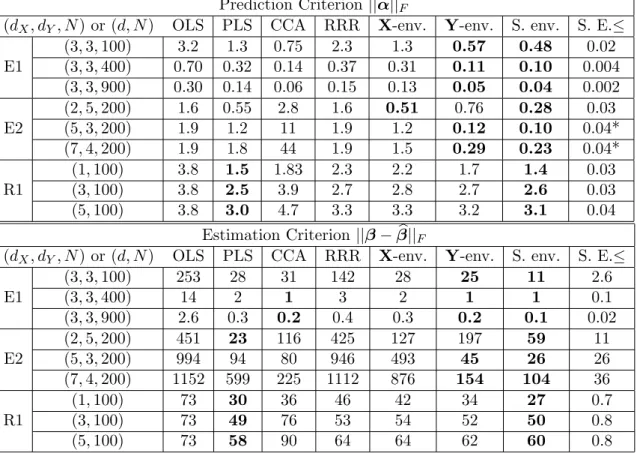
3.2 Prediction versus OLS for varying simultaneous envelope dimensions . . . . 48

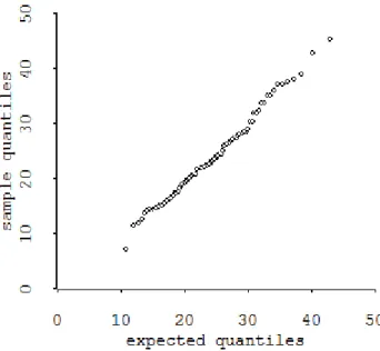
3.3 Probability plot of 1D algorithm estimator . . . 50

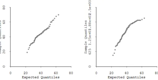
3.4 Probability plots based on 1D and SIMPLS algorithms . . . 51

3.5 Biscuit dough data . . . 53

4.1 Effect of rank and dimension . . . 81

4.2 Determining envelope dimensions . . . 82

4.3 Varying signal-to-noise and immaterial-to-material ratios . . . 83

4.4 Theoretical, bootstrap and actual standard errors . . . 84

5.1 Illustration of envelopes in logistic regression . . . 105

5.2 AIS data: heights and weights of male and female athletes . . . 124

(12)

Chapter 1

Introduction

1.1

Background and organization of this dissertation

An important topic in statistics is to reduce the dimensionality of data set and parameter space without losing any necessary information. There is a nascent area in dimension reduction called envelopes, whose goal is to increase efficiency in multivariate parameter estimation and prediction. This is achieved by enveloping the information in the data that is material to the estimation of the parameters of interest, while excluding the information that is immaterial to estimation. The reduction in estimative variation can be quite substantial when the immaterial variation is relatively large.

Envelopes were introduced by Cook, Li and Chiaromonte (2010) for response reduction in the multivariate linear model with normal errors. They showed that the asymptotic co-variance matrix of the envelope estimator of the regression coefficients is never larger than that of the usual maximum likelihood estimator and has the potential to be substantially smaller. When some predictors are of special interest, Su and Cook (2011) proposed the partial envelope model, with the goal of improving efficiency of the estimated coefficients corresponding to these particular predictors. Cook, Helland and Su (2013) used envelopes to study predictor reduction in multivariate linear regression and established a connection between envelopes and the SIMPLS algorithm (de Jong 1993; see also ter Braak and de Jong , 1998) for partial least squares regression. They showed that SIMPLS is based on a √n-consistent estimator of an envelope and, using this connection, they proposed an envelope estimator that has the potential to dominate SIMPLS in prediction. Still in the context of multivariate linear regression, Schott (2013) used saddle point approximations to improve a likelihood ratio test for the envelope dimension. Su and Cook (2013) adapted envelopes for the estimation of multivariate means with heteroscedastic errors, and Su and Cook (2012) introduced a different type of envelope construction, called inner envelopes, that can produce efficiency gains when envelopes offer no gains.

This dissertation deepens and broadens existing statistical theories and methodologies

(13)

in the envelope literature by making the following major achievements: (i) a fast and stable one-dimensional algorithm is proposed in Chapter 2 for estimating an envelope in general; (ii) in Chapter 3, we connect envelope methods with other popular methods for dimension reduction, and introduce envelopes for simultaneously reducing the predictors and responses in multivariate linear regression; (iii) in Chapter 4, we construct a hybrid method of reduced-rank regression and envelope models, and also illuminate such general applicable approach of combining the strength of envelopes and other methods; (iv) finally in Chapter 5, we break through the limitation of envelopes in multivariate linear models and introduce the novel constructive principle of enveloping an arbitrary parameter vector or matrix, based on a pre-specified asymptotically normal estimator.

1.2

Notations

The following notations and definitions will be used in our exposition. Matrices and subspaces.

Let Rm×n be the set of all real m×n matrices and letSk×k be the set of all real and

symmetric k×k matrices. Suppose M ∈ _Rm×n_{, then span(M)} _⊆

Rm is the subspace

spanned by columns of M. The Grassmann manifold consisting of the set of all u dimen-sional subspaces of Rr, u ≤ r, is denoted as Gu,r. We use PA(V) = A(ATVA)−1ATV

to denote the projection onto span(A) with the V inner product and use PA to denote

projection onto span(A) with the identity inner product. Let QA(V) = I−PA(V). We

will use operators vec : Ra×b → Rab, which vectorizes an arbitrary matrix by

stack-ing its columns, and vech : Ra×a → Ra(a+1)/2, which vectorizes a symmetric matrix by

stacking the unique elements of its columns. LetA⊗Bdenote the Kronecker product of two matrices A and B. The Kronecker product of two subspaces A and B is defined as A ⊗ B ={a⊗b|a ∈ A, b ∈ B}, which equals span(A⊗B) for any A and B such that A= span(A) andB= span(B). For anm×nmatrixAand ap×q matrixB, their direct sum is defined as the (m+p)×(n+q) block diagonal matrixA⊕B= diag(A,B). We will also use the⊕operator for two subspaces. IfS ⊆_Rp_and_{R ⊆}

RqthenS ⊕R= span(S⊕R)

where S and R are basis matrices for S and R. The sum of two subspaces S1 and S2 of

Rm is defined as S1+S2 ={v1+v2|v1∈ S1,v2∈ S2}.

Random vectors and their distributions.

For three arbitrary random vectors A, B and C, let A ∼ B denote that A has the same distribution as B, let A ⊥⊥ B denote that A is independent of B and let A ⊥⊥ B|C indicate that A is conditionally independent of B given C. In multivariate linear regression of Y on X: Y = α+βX+, we use ΣX and ΣY to denote the population

covariance matrices ofXandY, useΣXYto denote their cross-covariance matrix, and use

(14)

3

ΣY|X = ΣY −ΣT_XYΣ−_X1ΣXY. The sample counterparts of these population covariance

matrices are denoted bySX,SY,SXY,SY|XandSX|Y. Sample covariance matrices based

on an i.i.d. sample of (X1,Y1), . . . ,(Xn,Yn) are defined with the divisorn. For instance, SX =Pni=1(Xi−X)(Xi−X)T/n,SXY =Pni=1(Xi−X)(Yi−Y)T/nandSY|Xdenotes the

covariance matrix of the residuals from the linear fit ofYonX: SY|X=SY−SYXS−_X1SXY,

andSY◦X=SYXS−X1SXY denotes the sample covariance matrix of the fitted vectors from

the linear fit ofYonX. We also defineΣ_A|B andSA|B in the same way for two arbitrary

random vectors.

Estimation methods and some common abbreviations.

We use θb_α to denote an estimator of θ with known parameters α. If

√

n(θb−θ)

converges to a normal random vector with mean 0 and covariance matrix Φwe write its asymptotic covariance matrix as avar(√nθb) =Φ. Some commonly used abbreviations are:

AIC Akaike information criterion

BIC Bayesian information criterion

CCA Canonical correlation analysis

MLE Maximum likelihood estimator

OLS Ordinary least squares

PCA Principal component analysis

PLS Partial least squares. Also, SIMPLS and NIPALS are two popular algorithms for partial least squares (linear) regression, and IRPLS is the popular algorithm for partial least squares in generalized linear models.

RRR Reduced-rank regression

For a common parameter θ in different models, we will use subscripts to distinguish the estimators according to different models: θb_env for the envelope estimator, θb_OLS for the

ordinary least square estimator, θb_RE for the reduced-rank envelope estimator (a method

proposed in Chapter 4) andθb_RR for the reduced-rank regression estimator.

1.3

Envelope models and methods

In this section, we first review some key definition for envelopes and then illustrate the concepts by a simple data set from Kenward’s study (1987).

(15)

1.3.1 Definition of an envelope

This following definition of a reducing subspace is equivalent to the usual definition found in functional analysis (Conway 1990) and in the literature on invariant subspaces, but the underlying notion of reduction is incompatible with how it is usually understood in statistics. Nevertheless, it is common terminology in those areas and is the basis for the definition of an envelope (Cook, et al., 2010) which is central to our developments. Definition 1.1. A subspace R ⊆_Rd _{is said to be a reducing subspace of} _M_∈

Rd×d if R decomposes M as M=PRMPR+QRMQR. If R is a reducing subspace of M, we say thatR reduces M.

The next definition shows how to construct an envelope in terms of reducing subspaces. Definition 1.2. Let M∈_Sd _{and let} _{B ⊆}_span(M)_{. Then the} _M_{-envelope of} _B_{, denoted}

by E_M(B), is the intersection of all reducing subspaces of M that containB.

The intersection of two reducing subspaces ofMis still a reducing subspace ofM. This means that EM(B), which is unique by its definition, is the smallest reducing subspace

containing B. Also, the M-envelope of B always exist because of the requirement B ⊆ span(M). If span(U) = B, then we write E_M(U) := E_M(span(U)) = E_M(B) to avoid notation proliferation. LetE_M⊥(U) denote the orthogonal complement of EM(U).

The following proposition summarizes some key algebraic properties of envelopes in Cook et al. (2010). For a matrix M ∈ Sp×p, let λi and Pi, i = 1, . . . , q, be its distinct eigenvalues and corresponding eigen-projections so thatM=Pq

i=1λiPi. Define the

func-tion f∗ : Rp×p → Rp×p as f∗(M) = Pqi=1f(λi)Pi, where f : R→ R is a function such

thatf(x) = 0 if and only ifx= 0. Proposition 1.1. (Cook et al. 2010)

1. If M ∈ _Sp×p _has _q _≤ _p _{eigenspaces, then the} _M_{-envelope of} _{B ⊆} _span(M) _{can be}

constructed as EM(B) =Pq_i₌₁PiB;

2. With f and f∗ as previously defined,E_M(B) =E_M(f∗(M)B). 3. If f is strictly monotonic thenE_M(B) =E_f∗₍_M₎(B) =E_M(f∗(M)B).

From this proposition, we see that the M-envelope of B is the sum of the eigenspaces of M that are not orthogonal to B; that is, the eigenspaces of M onto which B projects non-trivially. This implies that the envelope is the span of some subset of the eigenspaces of M. In the regression context, Bis typically the span of a regression coefficient matrix or a matrix of cross-covariances, andMis chosen as a covariance matrix which is usually positive definite. We next illustrate the potential gain of envelope method using a linear regression example.

(16)

5

1.3.2 Concepts and methodology

We use Kenward’s (1987) data to illustrate the working mechanism of envelopes in multi-variate linear regression. These data came from an experiment to compare two treatments for the control of an intestinal parasite in cattle. Thirty animals were randomly assigned to each of the two treatments. Their weights (in kilograms) were recorded at the beginning of the study prior to treatment application and at 10 times during the study corresponding to weeks 2, 4, 6, ..., 18 and 19; that is, at two-weeks intervals except the last which was over a one-week interval. The goal was to find if there is a detectable difference between the two treatments and, if such a difference exists, the time at which it first occurred. As emphasized by Kenward (1987), although these data have a typical longitudinal structure, the nature of the disease means that growth during the experiment is not amenable to modeling as a smooth function of time, and that fitting growth profiles with a low degree polynomial may hide interesting features of the data because the mean growth curves for the two treatment groups are very close relative to their variation from animal to animal. Indeed, profile plots of the data suggest no difference between the treatments. Kenward modeled the data using a multivariate linear model with an “ante-dependence” covariance structure. Here we proceed with an envelope analysis based on a multivariate linear model, following the structure outlined by Cook et al. (2010).

Neglecting the basal measurement for simplicity, let Yi ∈ R10, i = 1, . . . ,60, be the

vector of weight measurements of each animal over time and let Xi = 0 or 1 indicate the two treatments. Our interest lies in the regression coefficientβfrom the multivariate linear regression Y=α+βX+, where it is assumed that ∼N(0,Σ_Y|X). Letβb_OLS denote

the ordinary least squares estimator ofβ, which is also the maximum likelihood estimator. The estimates and their residual bootstrap standard errors are shown in Table 1.1. The maximum absolutet-value over the elements ofβb_OLSis 1.30, suggesting that the treatments

do not have a differential affect on animal weight. However, with a value of 26.9 on 10 degrees of freedom, the likelihood ratio statistics for the hypothesis β = 0 indicates otherwise. We next turn to an envelope analysis.

Let Γ ∈ _R10×u _{be a semi-orthogonal basis matrix for} _E

ΣY|X(β), the ΣY|X-envelope

of span(β), and let (Γ,Γ0) be an orthogonal matrix. Then span(β) ⊆ EΣY|X(β) by

Definition 1.2 and we can express β =Γη, whereη ∈ _Ru×1 _{carries the coordinates of} _β

relative to the basis Γ and 1 ≤ u ≤ 10. Also, because span(Γ) is a reducing subspace of ΣY|X (Definition 1.1), the envelope version of the multivariate linear model can now be written as Y =α+ΓηX+, with Σ_Y|X =ΓΩΓT +Γ0Ω0ΓT0, where Ω∈Ru×u and

Ω0 ∈R(10−u)×(10−u)are positive definite matrices. Under this model,ΓT0Y|X∼ΓT0Yand

ΓT₀Y ΓTY|X. Consequently,ΓT₀Ydoes not respond to changes inXeither marginally or because of an association withΓTY. For these reasons we regard ΓT₀Y as the immaterial

(17)

information and ΓTY as the material information. Envelope analyses are particularly effective when the immaterial variation var(ΓT₀Y) is large relative to the material variation var(ΓTY). After finding a value Γb of Γ that minimizes the likelihood-based Grassmann

objective function log|ΓT_S−1

Y Γ|+ log|ΓTSY|XΓ|, which will be discussed in Section 2.2, over all semi-orthogonal matrices Γ ∈ R10×u, the envelope estimator of β is given by

b

βenv=P_Γ_bβb_OLS. Becauseu(10−u)≤25, the real dimensions involved in this optimization

are small and the envlp code can be used without running into computational issues. Standard methods like BIC and likelihood ratio testing can be used to guide the choice of the envelope dimension u. Both methods indicate clearly that u = 1 in this illustration. In other words, the treatment difference is manifested in only one linear combinationΓTY of the response vector.

The envelope estimateβb_env is shown in Table 1.1 along with bootstrap standard errors

and standard errors obtained from the asymptotic normal distribution of √n(βb_env −β)

by the plug-in method (See Cook et al. (2010) for the asymptotic covariance matrix). We see that the asymptotic standard errors are a bit smaller than the bootstrap standard errors. Using either set of standard errors and using a Bonferroni adjustment for multiple testing, we see that there is a difference between the treatments and that the difference is first manifested around week 10 and remains thereafter. As shown in the final row of Table 1.1, the bootstrap standard errors for the elements of βb_OLS were 2.2 to 5.9 times

those of βb_env. Hundreds of additional samples would be needed to reduce the standard

errors of the elements ofβb_OLS by these amounts.

We conclude this example by considering the regression of the 6th and 7th element of Y, corresponding to weeks 12 and 14, on X, now letting Y = (Y6, Y7)T. This allows

us to represent the regression graphically and thereby provide intuition on the working mechanism of an envelope analysis. Figure 1.1 shows a plot of Y6 versus Y7 with the

points marked by treatment. Sinceβ= E(Y|X = 1)−E(Y|X = 0)∈_R2×1_{, the standard}

estimator for β is obtained as the difference in the marginal means after projecting the data onto the horizontal and vertical axes of the plot. The two densities estimates with the larger variation shown along the horizontal axes of the plot represent this operation. These density estimates are nearly identical, which explains the relatively small t-values from the standard model mentioned previously. However, it is clear from the figure that the treatments do differ.

An envelope analysis infers that β= (β6, β7)T is parallel to the second eigenvector of

ΣY|X = cov(Y6, Y7). Hence by Proposition 1.1, EΣY|X(β) = span(β), as shown on the

plot. The envelope represents the subspace in which the populations differ, which seems consistent with the pattern of variation shown in the plot. The orthogonal complement of the envelope, represented by a dashed line on the plot, represents the immaterial variation. The two populations are inferred to be the same when projected onto this subspace, which

(18)

7

also seems consistent with the pattern of variation in the plot. The envelope estimator of a mean difference is obtained by first projecting the points onto the envelope and thus removing the immaterial variation, and then projecting the points onto the horizontal or vertical axis. The two density estimates with the smaller variation represent this operation. These densities are well separated, leading to increased efficiency.

240 260 280 300 320 340 360 260 280 300 320 340 360 Weight on week 12 Weight on week 14 Envelope ΓT Y E Γ₀T_Y E S

Figure 1.1: Kenward’s cow data with the 30 animals receiving one treatment marked as o’s and the 30 animals receiving the other marked as x’s.The curves on the bottom are densities of Y6|(X = 0) and Y6|(X = 1): the flat two curves are obtained by projecting

the data onto the Y6 axis (standard analysis), and the two other densities are obtained

by first project the data onto the envelope and then onto theY6 axis (envelope analysis).

Representative projection paths, labeled ‘E’ for envelope analysis and ‘S’ for standard analysis, are shown on the plot.

(19)

OLS estimator Week 2 4 6 8 10 12 14 16 18 19 b βOLS 2.4 3.3 3.1 4.7 4.7 5.5 -4.8 -4.5 -2.8 5.0 Bootstrap SE 2.9 3.2 3.5 3.6 4.0 4.2 4.4 4.5 5.4 6.0 Envelope estimator b βenv -2.2 -0.5 0.9 2.4 2.9 5.4 -5.1 -4.6 -3.7 4.2 Bootstrap SE 1.13 0.84 1.07 1.03 0.81 1.12 1.07 1.04 1.08 1.02 Asymptotic SE/√n 0.88 0.74 0.72 0.84 0.70 1.02 0.92 0.86 0.90 0.85

Bootstrap SE ratios of OLS estimator over envelope estimator

SE ratios 2.6 3.8 3.3 3.5 5.0 3.7 4.1 4.3 5.0 5.9

Table 1.1: Bootstrap standard errors of the 10 elements inβbunder the OLS estimator and

the envelope estimator with u = 1. The bootstrap standard errors were estimated using 100 bootstrap samples.

(20)

Chapter 2

Algorithms for Envelope

Estimation

2.1

Introduction

As mentioned earlier in Chapter 1, envelope methods aim to reduce estimative variation in multivariate linear models. The reduction is typically associated with predictors or responses, and can generally be interpreted as effective dimensionality reduction in the parameter space. Such reduction is achieved by enveloping the variation in the data that is material to the goals of the analysis while simultaneously excluding the immaterial vari-ation. Efficiency gains are then achieved by essentially basing estimation on the material variation alone. The improvement in estimation and prediction can be quite substan-tial when the immaterial variation is large, sometimes equivalent to taking thousands of additional observations.

All current envelope methods, for example Cook et al. (2010; 2013), are all likelihood-based. The likelihood-based approach to envelope estimation requires, for a given envelope dimension u, optimizing an objective function of the form f(Γ), where Γ is a k ×u, k > u, semi-orthogonal basis matrix for the envelope. The objective function satisfies f(Γ) = f(ΓO) for any u×u orthogonal matrix O. Hence the optimization is essentially over the set of allu-dimensional subspaces ofRk, which is a Grassmann manifold denoted

asG_u,k. Sinceu(k−u) real numbers are required to specify an element ofG_u,k uniquely, the optimization is essentially overu(k−u) real dimensions. In multivariate linear regression, k can be either the number of responses r or the number of predictors p, depending on whether one is pursuing response or predictor reduction.

All present envelope methods rely on the Matlab package sg min by Ross A. Lip-pert (_{http://web.mit.edu/~ripper/www/software/}) to optimize f(Γ). This package provides iterative optimization techniques on Stiefel and Grassmann manifolds, including

(21)

non-linear conjugate gradient (PRCG and FRCG) iterations, dog-leg steps and Newton’s method. For more background in Grassmann manifolds and Grassmann optimizations, see Edelman, Tomas and Smith (1998) and Absil, Mahony and Sepulchre (2008). Since Grass-mann manifold optimization is not popular in statistics, it is worth mentioning that there are two packages for sufficient dimension reduction methods using Grassmann manifold optimization: R packageGrassmannOptim by Adragni, Cook and Wu (2012) and Matlab packageLDRby Cook, Forzani and Tomassi (2011), which usessg minto implement several sufficient dimension reduction methods

To implement an envelope estimation procedure, one needs to specify the objective functionf(Γ) and its analytical first-order derivative function. Then given an initial value of Γ, this package will compute numerical second-order derivatives and iterate until con-vergence or the maximum number of iterations is reached. The Matlab toolbox envlp

by Cook, Su and Yang (http://code.google.com/p/envlp/) uses sg min to implement a variety of envelope estimators along with associated inference methods. The sg min

package works well for envelope estimation, but nevertheless, optimization is often com-putationally difficult for large values of u(k−u). At higher dimensions, each iteration becomes exponentially slower, local minima can become a serious issue and good starting values are essential. The envlptoolbox implements a seemingly different version of f(Γ) for each type of envelope, along with tailored starting values.

In this chapter we present two advances in envelope computation. First, we propose in Section 2.2 a model-free objective functionJn(Γ) for estimating an envelope and show that the three major envelope methods are based on special cases ofJn. This unifying objective function is to be optimized over the Grassmann manifold G_u,k, which for larger values of u(k−u) will be subject to the same computational limitations associated with speed, local minima and starting values. Second, we propose in Section 2.3 a fast one-dimensional (1D) algorithm that mitigates these computational issues. To adapt the envelope construction for relatively large values of u(k−u), we break down Grassmann optimization into a series of one-dimensional optimizations so that the estimation procedure is speeded up greatly, and starting values and local minima are no longer an issue. Although it may be impossible to break down a general u-dimensional Grassmann optimization problem, we rely on special characteristics of envelopes in statistical problems to achieve the breakdown of envelope estimation. The resulting 1D algorithm, which is easy-to-implement, stable and requires no initial value input, can be tens to hundreds times faster than the general Grassmann manifold optimization foru >1, while still providing a desirable√n-consistent envelope estimator. We will use special forms of the 1D algorithm to find initial values for the simultaneous envelope in Chapter 3 and for reduced-rank envelope in Chapter 4. The 1D algorithm we introduce in Section 2.3 is much more general than its use in those two chapters and is directly applicable beyond the multivariate linear regression context,

(22)

11

see Chapter 5. The rest of this chapter is organized as follows. Section 2.4 consists of simulation studies and a data example to further demonstrate the advantages of the 1D algorithm. Section 2.5 is a brief conclusion of this chapter. Proofs and technical details are included in the Section 2.6.

2.2

Objective functions for estimating an envelope

2.2.1 The objective function and its properties

In this section we propose a generic objective function for estimating a basis Γ of an arbitrary envelope EM(B) ⊆ Rd, where M ∈ Sd is a symmetric positive definite matrix.

Let B be spanned by a d×d matrix U so that E_M(B) = E_M(U). Because span(U) = span(UUT), we can always denote the envelope by E_M(U) for some symmetric matrix U ≥ 0. We propose the following generic population objective function for estimating E_M(U):

J(Γ) = log|ΓTMΓ|+ log|ΓT(M+U)−1Γ|, (2.2.1) whereΓ∈_Rd×u_{denotes a semi-orthogonal basis for elements in Grassmann manifold}_G

u,d, u is the dimension of the envelope, and u < d. We refer to the operation of optimizing (2.2.1) or its sample version given later in (2.2.2) as full Grassmann (FG) optimization. SinceJ(Γ) =J(ΓO) for any orthogonalu×umatrixO, the minimizerΓe= arg min_ΓJ(Γ)

is not unique. But we are interested only in span(Γ), which is unique as shown in thee

following proposition.

Proposition 2.1. Let Γe∈_Rd×u be a minimizer of J(Γ). Then span(Γ) =e E_M(U).

To gain intuition on how J(Γ) is minimized by anyΓe that spans the envelope E_M(U),

we let (Γ,Γ0)∈Rd×dbe an orthogonal matrix and decompose the objective function into

two parts: J(Γ) =J(1)_{(Γ) +}_J(2)_{(Γ), where}

J(1)(Γ) = log|ΓT_MΓ|_{+ log}_|ΓT

0MΓ0|,

J(2)(Γ) = log|ΓT_(M₊_U)−1_{Γ| −}_log_|ΓT

0MΓ0|

= log|ΓT₀(M+U)Γ0| −log|ΓT0MΓ0| −log|M+U|.

The first function J(1)(Γ) is minimized by any Γ that spans a reducing subspace of M. Minimizing the second functionJ(2)_{(Γ) is equivalent to minimizing log}_|ΓT

0(M+U)Γ0| −

log|ΓT

0MΓ0|, which is no less than zero and equals to zero whenΓT0UΓ0 = 0. ThusJ(2)(Γ)

is minimized by anyΓ such thatΓT₀UΓ0 = 0, or equivalently, span(U)⊆span(Γ). These

properties of J(1)(Γ) and J(2)(Γ) are combined by J(Γ) to get a reducing subspace of M that contains span(U). In the context of multivariate linear regression, minimizingJ(2)(Γ) is related to minimizing the residual sum of squares and minimizingJ(2) is in effect pulling

(23)

the solution towards principal components of responses or predictors. Finally, because u is the dimension of the envelope, the minimizer span(Γ) is unique by Definition 1.2.e

The sample version Jnof J based on a sample of sizenis constructed by substituting estimatorsMc and Ub of Mand U:

Jn(Γ) = log|ΓTMΓ|c + log|ΓT(cM+U)b −1Γ|. (2.2.2)

Proposition 2.1 shows Fisher consistency of minimizers from optimizing the population objective function. Furthermore, √n-consistency of Γb = arg min_ΓJ_n(Γ) is stated in the

following proposition.

Proposition 2.2. Let Mc and Ub denote

√

n-consistent estimators forM>0and U≥0. Let Γb ∈_Rd×u be a minimizer of J_n(Γ), then P

b

Γ is

√

n-consistent for the projection onto

E_M(U).

When we connect the objective functionJn(Γ) with multivariate linear models in Sec-tion 2.2.2, we will find that previous likelihood-based envelope objective funcSec-tions can be written in form (2.2.2). The likelihood approach to envelope estimation is based on nor-mality assumptions for the conditional distribution of the response given the predictors or the joint distribution of the predictors and responses. The envelope objective function aris-ing from this approach is a partially maximized log-likelihood obtained broadly a follows. After incorporating the envelope structure into the model, partially maximize the normal log-likelihood functionLn(ψ,Γ) over all the other parametersψ withΓ fixed. This leads to a likelihood-based objective functionLn(Γ), which equals a constant plus−(n/2)Jn(Γ) with cM and Ub depending on context. Proposition 2.2 indicates that the function J_n(Γ)

can be used as a generic moment-based objective function requiring only √n-consistent matricesMc andU. Consequently, normality is not a requirement for estimators based onb

Jn(Γ) to be useful, a conclusion that is supported by previous work and by our experience. FG optimization ofJn(Γ) can be computationally intensive and can require a good initial value. The 1D algorithm in Section 2.3 mitigates the computational issues.

2.2.2 Connections with previous work

Envelope applications have so far been mostly restricted to the homoscedastic multivariate linear model

Yi =α+βXi+εi, i= 1, . . . , n, (2.2.3) where Y ∈ _Rr_{, the predictor vector} _X _∈

Rp, β ∈ Rr×p, α ∈ Rr and the errors εi are independent copies of the normal random vector ε ∼ N(0,ΣY|X). The maximum

(24)

13

Response envelopes

Cook, et al. (2010) studied response envelopes for estimation of the coefficient matrix

β. They conditioned on the observed values of X and motivated their developments by allowing for the possibility that some linear combinations of the response vector Y are immaterial to the estimation of β, as described previously in Section 1.3.2. Reiterating, suppose that there is an orthogonal matrix (Γ,Γ0)∈Rr×r so that (i) span(β)⊆span(Γ)

and (ii) ΓTY ΓT₀Y | X. This implies that (Y,ΓTX) ΓT₀X and thus that ΓT₀X is immaterial to the estimation of β. The smallest subspace span(Γ) for which these conditions hold is theΣY|X-envelope of span(β), EΣY|X(β).

To determine the FG estimator of E_Σ_Y_|_X(β), we let Mc = S_Y_|_X and Mc+Ub =S_Y in

the objective functionJn(Γ) to reproduce the likelihood-based objective function in Cook et al. (2010). Then the maximum likelihood envelope estimators are βb_env = P

b

Γβb and b

Σ_Y|X,env=PbΓSY|XPΓb+QΓbSY|XQΓb, whereΓb = arg minJn(Γ). Assuming normality for

εi, Cook et al. (2010) showed that the asymptotic variance of the envelope estimatorβb_env

is no larger than that of the usual least squares estimatorβb. Under the weaker condition

thatεi are independent and identically distributed with finite fourth moments, the sample covariance matricesMc and Ub are

√

n-consistent for M=Σ_Y|X and U =ΣY−ΣY|X = βΣ−_X1βT. By Proposition 2.2, we have √n-consistency of the envelope estimator βb_env

under this weaker condition.

Partial envelopes

Su and Cook (2011) used theΣ_Y|X-envelope of span(β1),EΣY|X(β1), to develop a partial

envelope estimator of β1 in the partitioned multivariate linear regression

Yi=α+βXi+εi =α+β1X1i+β2X2i+εi, i= 1, . . . , n, (2.2.4) where β1 ∈ Rr×p1, p1 ≤ p, is the parameter vector of interest, X = (XT1,XT2)T, β =

(β1,β2) and the remaining terms are as defined for model (2.2.3). In this formulation, the

immaterial information is ΓT₀Y, where Γ0 is a basis for EΣ⊥Y|X(β1). Since EΣY|X(β1) ⊆

EΣY|X(β), the partial envelope estimatorβb1,env=PΓbβb1has the potential to yield efficiency gains beyond those for the full envelope, particularly when E_Σ_Y_|_X(β) = Rr so the full

envelope offers no gain. In the maximum likelihood estimation ofΓ, the same forms ofM,c b

Uand Jn(Γ) are used for partial envelopesEΣY|X(β1), except the roles ofY andXin the

usual response envelopes are replaced with the residuals: R_Y|X2, residuals from the linear fits of Y on X2, and RX1|X2, the residuals of X1 on X2. Setting Mc = SRY|X₂|RX₁|X₂ =

S_Y|X and Mc +Ub = S_Y_|_X₂ in the objective function J_n(Γ) reproduces the likelihood

objective function of Su and Cook. Again, Proposition 2.2 gives √n-consistency without normality.

(25)

Predictor envelopes

Cook, et al. (2013) studied predictor reduction in model (2.2.3), except the predictors are now stochastic with var(X) =ΣXand (Y,X) was assumed to be normally distributed for

the construction of maximum likelihood estimators. Their reasoning, which parallels that for response envelopes, lead them to parameterize the linear model in terms of E_Σ_X(βT) and to achieve similar substantial gains in the estimation of β and in prediction. The immaterial information in this setting is given by ΓT₀X, where Γ0 is now a basis for

E⊥

ΣX(β

T_{). They also showed that the SIMPLS algorithm for partial least squares provides} a √n-consistent estimator of EΣX(β

T_{) and demonstrated that the envelope estimator}

b

βenv =βbPT

b

Γ(SX)

typically outperforms the SIMPLS estimator in practice. For predictor reduction in model (2.2.3), the envelopeEΣX(β

T_{) is estimated with}

c

M=S_X|Y,Mc+Ub =

SX. As with response and partial envelopes, Proposition 2.2 gives us

√

n-consistency without requiring normality for (Y,X).

Techniques for estimating the dimension of an envelope are discussed in the parent ar-ticles of these methods, including use of an information criterion like BIC, cross validation or a hold-out sample.

2.2.3 New envelope estimators inspired by the objective function

The objective function Jn(Γ) can also be used for envelope estimation in new problems. For example, to estimate the multivariate mean µ∈_Rr _{in the model} _Y₌_µ₊_ε_{, we can} use theΣY-envelope of span(µ) by takingM=ΣYandU=µµT, whose sample versions

are: cM = S_Y, Ub = µ_bµ_bT and µ_b = n−1 Pn

i=1Yi. Then substituting cM and Ub leads to

the same objective function Jn(Γ) as that obtained when deriving the likelihood-based envelope estimator from scratch.

For the second example, let Yi ∼ Nr(µ,ΣY), i = 1, . . . , n, consist of longitudinal

measurements of n subjects over r fixed time points. Suppose we are not interested in the overall mean µ = 1T_rµ/r ∈ _R1 _{but rather interest centers on the deviations at}

each time point α = µ−µ1r ∈ Rr. Let Q1 = Ir−1r1Tr/r denote the projection onto the orthogonal complement of span(1r). Then α = Q1µ and we consider estimating

the constrained envelope: E_Q₁_Σ_Y_Q₁(Q1µµTQ1) :=EM(U). Optimizing Jn(Γ) withMc =

Q1SYQ1andUb =Q₁µ_bµ_bTQ₁will again lead to the maximum likelihood estimator and to

√

n-consistency without normality. Later from Proposition 2.3, we will see that E_M(U) = Q1EΣY(µµ

T_{) and the optimization can be simplified.}

The objective function Jn(Γ) introduces also a way of extending envelope regression semi-parametrically or non-parametrically. This can be done by simply replacing the sam-ple covariances cMandUb in Section 2.2.2 with their semi-parametric and non-parametric

counterparts. Given a multivariate model Y = f(X) +, where β ∈ _Rp_, _Y _∈

(26)

15

f(·) : _Rp _→

Rr, the envelope for reducing the response can be estimated by taking cM

equal to the sample covariance of the residuals: Mc=n−1 Pn

i=1{Yi−bf(X_i)}{Y_i−bf(X_i)}T,

and cM+Ub =S_Y.

2.3

A 1D algorithm

In this section we propose a method for estimating a basis Γ of an arbitrary envelope E_M(B)⊆_Rd _{based on a series of one-dimensional optimizations. The resulting algorithm} is fast and stable, does not require carefully chosen starting values and the estimator it produces converges at the root-n rate. The estimator can be used as it stands, or as a √

n-consistent starting value for (2.2.2). In the latter case, one Newton-Raphson step from the starting value provides an estimator that is asymptotically equivalent under normality to the maximum likelihood estimators discussed in Section 2.2.2 (Lehmann and Casella, 1998, p. 454.) The algorithm we present here can also be used for finding initial values of simultaneous envelope objective function in Chapter 3 and initial values of reduced-rank envelope objective function in Chapter 4.

The population algorithm described in this section extracts one dimension at a time from EM(B) = EM(U) until a basis is obtained. It requires only M > 0, U ≥ 0 and

u = dim(E_M(B)) as previously defined in Section 2.2. Sample versions are obtained by substituting√n-consistent estimatorsMc and Ub for Mand U. Otherwise, the algorithm

itself does not depend on a statistical context, although the manner in which the estimated basis is used subsequently does.

The following proposition is the basis for a sequential breakdown of a u-dimensional FG optimization.

Proposition 2.3. Let (B,B0) denote an orthogonal basis of Rd, where B∈ Rd×q, B0 ∈

Rd×(d−q) and span(B)⊆ EM(B). Then v∈ EBT

0MB0(B

T

0B) implies that B0v∈ EM(B).

Suppose we know an orthogonal basis B for a subspace of the envelope E_M(B). Then by Proposition 2.3 we can find the rest ofEM(B) by looking intoEBT

0MB0(B

T

0B), which is

a lower dimensional envelope. This then provides a motivation for Algorithm 1, which sequentially constructs vectors gk ∈ EM(B), k = 1, . . . , u, until a basis is obtained,

span(g1, . . . ,gu) =EM(B). This algorithm follows the structure implied by Proposition 2.3

and the stepwise objective functionsDk are each one-dimensional versions of (2.2.1). The first directiong1 requires optimization inRd, while the optimization dimension is reduced

by 1 in each subsequent step.

Remark 1. At step 2(c) of Algorithm 1, we need to minimize the stepwise objective function Dk(w) under the constraint that wTw = 1. The sg min package can still be used to deal with this constraint since we are optimizing over one-dimensional Grassmann

(27)

Algorithm 1 The 1D algorithm. 1. Set initial valueg0 =G0= 0.

2. Fork= 0, . . . , u−1,

(a) LetGk= (g1, . . . ,gk) ifk≥1 and let (Gk,G0k) be an orthogonal basis forRd.

(b) Define the stepwise objective function

Dk(w) = log(wTMkw) + log{wT(Mk+Uk)−1w}, (2.3.1) whereMk=GT0kMG0k,Uk =GT0kUG0k and w∈Rd−k.

(c) Solvewk+1 = arg minwJk(w) subject to a length constraint wTw= 1. (d) Definegk+1=G0kwk+1 to be the unit length (k+ 1)-th stepwise direction.

manifolds. An alternative way is to integrate the constraintwTw= 1 into the objective function in (2.3.1), so that we only need to minimize the unconstrained function

e

Dk(w) = log(wTMkw) + log{wT(Mk+Uk)−1w} −2 log(wTw), (2.3.2) with an additional normalization step for its minimizer wk+1 ← wk+1/||wk+1||. This

unconstrained objective functionDk(w) can be solved by any standard numerical methods such as conjugate gradient or Newton’s method. We have implemented this idea with the general purpose optimization functionoptim in R and obtained good results.

Remark 2. We have also considered other types of sequential optimization methods for envelope estimation. For example, we considered minimizing D1(w) at each step under

orthogonality constraints such aswT_k₊₁wj = 0 or w_kT₊₁Mwj = 0 for j ≤k. These types of orthogonality constraints are used widely in PLS algorithms and principal components analysis. We find the statistical properties of these sequential methods are inferior to those of the 1D algorithm. For instance, they are clearly inferior in simulations and we doubt that they lead to consistent estimators.

The next two propositions establish the Fisher consistency of Algorithm 1 in the pop-ulation and the√n-consistency of its sample version.

Proposition 2.4. Assume thatM>0, and letGu denote the end result of the algorithm.

Thenspan(Gu) =EM(B).

Proposition 2.5. Assume that M > 0 and let Mc > 0 and Ub denote

√

n-consistent estimators for M and U. Let Gb_u denote the estimator obtained from the 1D algorithm using Mc and Ub instead of Mand U. Then P

b

Gu is

√

n-consistent for the projection onto

(28)

17

The algorithm discussed in this section can be used straightforwardly in the contexts of the three envelopes reviewed in Section 2.2.2 and the extensions sketched in Section 2.2.3. The statistical properties of the 1D algorithm estimator stated in Propositions 2.4 and 2.5 are exactly parallel to the properties of FG optimization in Propositions 2.1 and 2.2.

2.4

Simulations

In this section, we compare the 1D algorithm to FG (full Grassmann manifold) optimiza-tion, focusing on computational cost. For fair comparisons, the implementation of our 1D algorithm was based on minimizing the length-constrained objective function (2.3.1) using

the sg min package. Implementation of the 1D algorithm with other computing

pack-ages using the unconstrained objective function (2.3.2) may offer even faster estimation procedures.

2.4.1 Simulations

We considered the response envelope model in Cook et al. (2010) with univariate predictor X ∼ N(0,1) and multivariate response Y = α+βX +, where ∼ Nr(0,ΣY|X) and we were interested in estimation of E_Σ

Y|X(β). We generated M = ΣY|X and U = ββ

T in accordance with an envelope structure: β = Γη and ΣY|X = ΓΩΓT +Γ0Ω0ΓT0 for

some positive definite matricesΩ∈_Su _and _Ω

0∈Sr−u and a vector of onesη=1u ∈Ru.

The semi-orthogonal basisΓ∈Rr×u forEM(U) was randomly generated andΓ0 was then

obtained so that (Γ,Γ0) was an orthogonal basis for Rr. The two covariance matrices

Ω, Ω0 were generated as AAT > 0, where A was a square matrix with corresponding

dimensions and was filled with uniform (0,1) random numbers.

We first examined the performances of our 1D algorithm in the population. We gen-erated 100 pairs of Mand U for each of three dimension configurations, (r, u) = (10,3), (r, u) = (30,10) and (r, u) = (70,20). These dimensions correspond to the real optimiza-tion dimensionsu(r−u) = 21, 200 and 1000 for FG optimization, while the 1D algorithm optimizes over at mostr−1 real dimensions at each iteration. We recorded the CPU time T for estimating an envelope and the Frobenius norm between the true envelope and an estimated envelope defined as dist(Γ,eΓ) =||ΓΓT−ΓeΓeT||_F. The results for running the 1D

algorithm (Algorithm 1) and the FG optimization of (2.2.2) are given in the first three rows of Table 2.1. Apparently the 1D algorithm achieved the same accuracy as FG optimization and was much less time-consuming, especially at the large dimension (r, u) = (30,10) and (r, u) = (70,20).

We next generated 100 replicated data sets for one pairs of M and U, and used the sample estimatorcM=S_Y_|_X andUb =S_Y−S_Y_|_X for envelope estimation. We letn= 400

(29)

FG optimization in terms of computational efficiency.

For FG optimization, we chose initial value according to the approach described in Su and Cook (2011; Section 3.5), first optimizing the objective function over the 2r eigenvec-tors ofMc andMc+U. This initial value search procedure alone could be computationallyb

costly, but we did not include the time spent on this when we summarized the computing time T for the FG optimization algorithm in Table 2.1. Additionally, we used only the true value of u in each simulation. The performance of optimizations at other than the true value ofu, as necessary in the application of BIC, need not follow those of Table 2.1, as we illustrate in the next section.

1D algorithm FG optimization T dist(Γ,Γ)b T dist(Γ,Γ)b (n, r, u) = (∞,10,3) 2.0 (0.2) <1.0×10−8 6.6 (0.3) <1.0×10−8 (n, r, u) = (∞,30,10) 2.6 (0.1) <1.0×10−4 _{127 (11)} _<_1.0_×₁₀−4 (n, r, u) = (∞,70,20) 447 (11) <1.0×10−2 _{5084 (1283)} _<_1.0_×₁₀−2 (n, r, u) = (400,10,3) 0.6 (0.04) 1.1 (0.05) 1.2 (0.09) 1.0 (0.05) (n, r, u) = (400,30,10) 30.7 (0.6) 2.8 (0.02) 121 (7) 3.1 (0.02) (n, r, u) = (400,70,20) 534 (5) 4.6 (0.04) 4187 (68) 4.7 (0.03) Table 2.1: Comparisons between the 1D algorithm and FG optimization. Each cell contains the average running time in seconds over 100 simulations, with its standard error given in parentheses. The population algorithms with M and U were indicated with n=∞ and the sample algorithms had n= 400.

2.4.2 Starting values

As mentioned previously, good starting values can be crucial to the performance of FG optimization. To highlight this point, we used the meat data analyzed previously by Cook et al. (2013) for envelope predictor reduction in multivariate linear regression. This data set consists of spectral measurements from infrared transmittance for fat, protein and water for 103 meat samples. Following Cook et al. (2013), we used the protein percentage as the univariate response. The p = 50 predictors were spectral measurements at every fourth wavelength between 850nm and 1050nm. Using five-fold cross-validation prediction error as their criterion andu varying from 1 to 25, Cook et al. (2013) compared the FG envelope estimator described in Section 2.2.2 to the OLS and SIMPLS estimators. The starting value for the FG envelope estimator was the SIMPLS estimator, which is √ n-consistent in the context of predictor envelopes and had better performance than OLS. SIMPLS was designed specifically for predictor reduction and is not applicable to response or partial reduction or to the extensions discussed in Section 2.2.3. Their results showed the envelope estimator to be uniformly superior to OLS, superior to SIMPLS for small values of u and about the same as SIMPLS for large values of u. In this study we used

(30)

19

the same setup as Cook et al. (2013), except we focused on comparisons between the 1D algorithm and the FG envelope estimator with starting values again chosen following the approach described in Su and Cook (2011; Section 3.5), since the 2r eigenvectors of cM

and cM+Ub may be all that is easily available without recourse to the 1D algorithm.

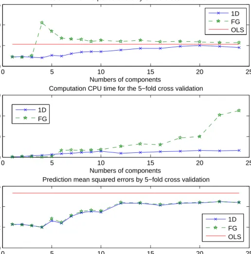
We plotted in Figure 2.1 (top two plots) the five-fold cross-validation squared prediction error and the elapsed CPU time (in seconds) for computing the FG envelope estimators with dimensions u = 1, . . . ,25. Although we had five-folds and thus estimated five en-velopes for each dimensionu, the time reported is the average for estimating one envelope. The number of real optimization dimensions u(50−u) varied between 49 and 625. For the larger values of u, FG optimization took a very long time to compute, so we capped the number of allowed iterations at 5000. For small dimensions, u ≤3, FG optimization and the 1D algorithm had close prediction performance, and there were no convergence issues. Foru= 4 and 5, FG optimizations tended to become trapped into local minima, as indicated by the prediction error. For larger dimensions, u >10, FG optimization began bumping into the iteration limit. The computation time for the 1D method was almost linearly increasing inubecause of the sequential manner of the algorithm. With increasing number of components, the prediction errors of both methods converged towards that of the ordinary least squares estimator as expected, since they both reduce to ordinary least squares whenu= 50. However, the 1D algorithm provided better estimators, consistently overu, than the OLS estimator and the FG envelope estimator.

This difference in the results reported by Cook et al. (2013) and the results shown in the top plot of Figure 2.1 arises because of the different staring values. In Cook et al. (2013), the initial values were √n-consistent, while here we chose initial values from the eigenvectors of Mc and Mc+U. When using these starting values, FG optimizationsb

tended to get trapped by local minima that were close to the initial values, which accounts for the inferior performance of the FG envelope estimator in this setting. From Lehmann and Casella (1998; Theorem 4.3), we know that one Newton-Raphson iteration from any √

n-consistent estimator, the 1D algorithm estimator for instance, will be asymptotically equivalent to the MLE, even if there were local minima. We used 100 iterations (instead of one) for the FG optimization with 1D algorithm estimators as initial values. The cross-validation prediction errors, shown in the bottom plot of Figure 2.1, were very close to those of the 1D algorithm. The FG algorithm did a little bit worse than the 1D algorithm at some u because with 100 iterations it occasionally got trapped in a local minimum as it tried to improve the starting value.

(31)

0 5 10 15 20 25 0 5 10 15 Numbers of components

Prediction mean squared errors

Prediction mean squared errors by 5−fold cross validation

1D FG OLS 0 5 10 15 20 25 0 200 400 600 Numbers of components CPU time

Computation CPU time for the 5−fold cross validation

1D FG 0 5 10 15 20 25 0 2 4 6 Numbers of components

Prediction mean squared errors

Prediction mean squared errors by 5−fold cross validation

1D FG OLS

Figure 2.1: Meat protein data. The FG optimizations shown in the top and the middle plots were based on starting values suggested by Cook and Su (2011; Section 5.3). And the FG optimization in bottom plot was using the 1D algorithm estimators as starting value.

(32)

21

2.5

Conclusion

Our study led to the following conclusions. The FG envelope estimator (2.2.2) can be computed straightforwardly when the number of real dimensions u(k−u) is relatively small, say less than 150, as illustrated in the example of Section 1.3.2. When this dimension is large, computing time and local minima can become serious issues, and then root-n consistent starting values become crucial. The 1D algorithm can be used confidently for starting values, or as a stand-alone algorithm for envelope estimation.

2.6

Proofs

2.6.1 Proposition 2.1

The proof of this proposition is very similar to the proof of Proposition 4.2 in Cook et al. (2013), thus is omitted.

The proof follows from Proposition 2.6 and Proposition 2.7 in the same way as Proposi-tion 2.5 in SecProposi-tion 2.6.5. Thus we omit the details of the proof.

Proof. From our set-up, we know thatBTMB>0 thus E_BT_MB(BTB) exists. LetΓ be a

basis ofE_M(B), and (Γ,Γ0) be a orthogonal basis ofRp, thenM=ΓΩΓT +Γ0Ω0ΓT0 and

B ⊆span(Γ) for some symmetric matrices Ω>0 andΩ0 >0. Therefore,

BT₀MB0 = (BT0Γ)Ω(BT0Γ)T + (BT0Γ0)Ω0(BT0Γ0)T

BT₀B ⊆ span(BT₀Γ), (2.6.1)

where span(BT₀Γ) is the orthogonal compliment of span(BT₀Γ0) in Rp−q since span(B) ⊆

span(Γ). Then we see that

BT₀MB0=PBT 0ΓB T 0MB0PBT 0Γ+QBT0ΓB T 0MB0QBT 0Γ, (2.6.2) which implies that span(BT₀Γ) is a reducing subspace of BT₀MB0 which also contains

BT₀B by (2.6.1). By definition, we know that E_BT

0MB0(B

T

0B) is the smallest reducing

subspace of BT₀MB0 that contains BT0B. Hence EBT

0MB0(B T 0B) ⊆ span(BT0Γ). Thus v∈ E_BT 0MB0(B T 0B) impliesB0v∈ EM(B).

(33)

Proof. We first write

M = ΓΦΓT +Γ0Ω0ΓT0,

M+U = ΓΩΓT +Γ0Ω0ΓT0,

where Ω0 > 0, Ω > 0, Φ > 0, Ω−Φ ≥ 0, Γ is semi-orthogonal basis for EM(B) and

(Γ,Γ0)∈Rp is orthogonal basis for Rp.

We begin by considering optimization for the first direction g1 = arg ming∈_RpD₀(g),

whereD0(g) = log(gTMg) + log{gT(M+U)−1g} and the minimization is subject to the

constraint gTg= 1. Let g =Γh+Γ0h0 for some h∈Ru and h0 ∈R(p−u). Consider the

optimization problem as the unconstrained problem, g1= arg min

g∈Rp

log(gTMg) + log{gT(M+U)−1g} −2 log(gTg) .

Then we will have the same solution as the original problem up to an arbitrary scaling constant. Next, we plug-in these expressions for g,M+U and M,

log(gTMg) + log{gT(M+U)−1g} −2 log(gTg) = log{hTΦh+hT₀Ω0h0}+ log{hTΩ−1h+hT0Ω

−1

0 h0} −2 log{hTh+hT0h0}

≡ f(h,h0).

Taking partial derivative with respect to h0, we have

∂ ∂h0 f(h,h0) = 2Ω0h0 hT_Φh₊_hT 0Ω0h0 + 2Ω −1 0 h0 hT_Ω−1_h₊_hT 0Ω −1 0 h0 − 4h0 hT_h₊_hT 0h0 .

To get local minimums we need to set _∂∂_h

0f(h,h0) = 0 which gives the following equality. 2Ω0 hT_Φh₊_hT 0Ω0h0 + 2Ω −1 0 hT_Ω−1_h₊_hT 0Ω −1 0 h0 h0 = 4 hT_h₊_hT 0h0 h0. Define A0 = 2Ω0 hT_Φh₊_hT 0Ω0h0 + 2Ω −1 0 hT_Ω−1_h₊_hT 0Ω −1 0 h0 / 4 hT_h₊_hT 0h0 . (2.6.3)

Since Ω0 >0, we know A0 >0. Then A0h0 =h0 has solutions only as eigenvectors

of A0. The eigenvectors of A0 are the same as those of Ω0. Hence, h0 equals 0 or any

eigenvector `k(Ω0) of Ω0. Therefore, the minimum value of f(h,h0) has to be obtained

by 0 or `k(Ω0) (since h0 =∞ can be easily eliminated). If h0 = 0 then our conclusion

follows.

Assume h0 6= 0 and Ω0h0=λkh0. Then,

f(h,h0) = log{ hTΦh+λkhT0h0 hT_h₊_hT 0h0 }+ log{h T_Ω−1_h₊ 1 λkh T 0h0 hT_h₊_hT 0h0 } = log{h T_Φh hT_h Wh+λk(1−Wh)}+ log{ hT_Ω−1_h hT_h Wh+ 1 λk (1−Wh)},

(34)

23

whereWh = h

T_h

hT_h₊_hT

0h0 is the weight between 0 and 1. Because log() is concave, we have log(aWh+b(1−Wh))≥Whlog(a) + (1−Wh) log(b). Hence,

f(h,h0) ≥ Wh logh T_Φh hT_h + log hT_Ω−1_h hT_h + (1−Wh) log(λk) + log( 1 λk ) = Wh logh T_Φh hT_h + log hTΩ−1h hT_h ≥ Wh·min h∈Rd logh T_Φh hT_h + log hTΩ−1h hT_h ≥ min h∈_Rd logh T_Φh hT_h + log hTΩ−1h hT_h .

The last inequality holds because

min h∈Rd logh T_Φh hT_h + log hTΩ−1h hT_h <0, (2.6.4)

which is proved in Section 2.6.4.

Moreover, the lower bound of f(h,h0), which is negative, will be attained if we let

Wh = 1 and let h = arg minh∈_Rd

n

logh_hTTΦh_h + log

hT_Ω−1_h

hT_h

o

. So we have the minimum found at Wh = h

T_h

hT_h₊_hT

0h0 = 1, or equivalently, g=Γh∈span(Γ).

For the (k+ 1)-th direction, gk+1 = G0kwk+1 where wk+1 = arg minw∈_Rp−kD_k(w),

subject towTw= 1.BecauseDk(w) = log(wTGT₀_kMG0kw)+log[wT

GT₀_k(M+U)G0k −1

w] has the same form asf(g), analogous to the first direction, this giveswk+1 ∈ EGT

0kMG0k(G

T

0kB). Thereforegk+1 =G0kwk+1 ∈ EM(B) by Proposition 2.3.

Proof of inequality (2.6.4) We first show that min_h∈Rd

n

logh_hTTΦh_h + log

hT_Ω−1_h

hT_h

o

≤ 0, then we assume the equality to conduct the proof by contradiction. Define the following two functions,

F(h;Φ,Ω−1) := logh T_Φh hT_h + log hTΩ−1h hT_h , F(h;Ω,Ω−1) := logh T_Ωh hT_h + log hT_Ω−1_h hT_h ,

Recall that Ω−Φ ≥ 0, hence F(h;Φ,Ω−1) ≤ F(h;Ω,Ω−1) for any h. Consider the minimum of both F(h;Φ,Ω−1) and F(h;Ω,Ω−1), we have

min

h F(h;Φ,Ω

−1₎_≤_min

h F(h;Ω,Ω

−1_{) = 0,}

where the minimum of the right hand side is zero by taking h equals to any eigenvector ofΩ.

Now we assume that minhF(h;Φ,Ω−1) = 0. Then for an arbitraryh,

(35)

Lethi=`i(Ω),i= 1, . . . , u, be thei-th unit eigenvector of Ωand plughi into the above inequalities, we have

0≤F(hi;Φ,Ω−1)≤F(hi;Ω,Ω−1) = 0, i= 1, . . . , u, which implies

0 = F(hi;Φ,Ω−1) = F(hi;Ω,Ω−1) = 0, i= 1, . . . , u, and more explicitly,

log(hT_iΦhi) = log(hTi Ωhi), i= 1, . . . , u, which implies Φ = Ω because that Φ, Ω ∈ _Ru×u _and _h

i, i = 1, . . . , u, are u linear independent vectors. Then by definitionU=ΓT_(Φ−_Ω)Γ_{= 0 leads to contradiction with} the dimension of the envelope.

Proof. Our proof of√n-consistency hinges on Amemiya’s (1985) results on the asymptotic properties of extremum estimators. Proposition 4.1.1 and Proposition 4.1.3 in Amemiya (1985) can be applied to our context. We first state these results and then sketch how they can be used to prove the √n-consistency for our algorithm.

Let Qn(y,θ) be a real-valued function of the random variablesy= (y1, . . . ,yn)T and the parametersθ= (θ1, . . . ,θK)T. We shall sometimes write Qn(y,θ) more compactly as Qn(θ). Let the parameter space beΘand let the true value ofθbeθtwhich is inΘ. Then Proposition 4.1.1 and Proposition 4.1.3 in Amemiya (1985) give asymptotic properties of the extremum estimator, θb_n = arg max_θ_∈_ΘQ_n(y,θ). We summarize the conditions in

Amemiya’s Propositions as follows.

(A) The parameter spaceΘis a compact subset of RK;

(B) Qn(y,θ) is continuous inθ ∈Θ; for all y and is a measurable function of y for all

θ∈Θ;

(C) n−1Qn(θ) converges to a nonstochastic function Q(θ) in probability uniformly in

θ∈Θ asngoes to infinity, andQ(θ) attains a unique global maximum at θt; (D) ∂2Qn(θ)/∂θ∂θT exists and is continuous in an open, convex neighborhood of θ0;

(E) n−1∂2Qn(y,θ)/∂θ∂θT _θ₌_θ∗

n converges to a finite nonsingular matrix

A(θt) = lim n→∞Eθt n−1∂2Qn(θ)/∂θ∂θT ,

(36)

25 (F) n−1/2{∂Qn(θ)/∂θ}_θ₌_θt →N(0,B(θt)), where B(θt) = lim n→∞Eθt n−1{∂Qn(θ)/∂θ} ∂Qn(θ)/∂θT .

Proposition 2.6. Under assumptions (A)-(C), θb_n converges to θ_t in probability.

Proposition 2.7. Under assumptions (A)-(F),√n(θb_n−θ_t)→N(0,A(θ_t)−1B(θ_t)A(θ_t)−1).

In our adaptation of Proposition 2.6 and Proposition 2.7, we let θ ≡ g whose true value is denoted by gt and let the random variables y = vech(M,c U). The parameterb

space is the 1D manifold Θ=G₍_p,₁₎ which is a compact subset of Rp, so condition (A) in

Proposition 2.6 is satisfied. The function to be maximized is defined as follows.

Qn(g) =−n/2 log(gTMg)c −n/2 log(gT(Mc+U)b −1g) +nlog(gTg). (2.6.5)

Condition (B) then holds. We next verify condition (C) that n−1Qn(g) converges uni-formly to

Q(g) =−1/2 log(gTMg)−1/2 log(gT(M+U)−1g) + log(gTg). (2.6.6) We have shown that the population objective function Q(g) attains the unique global maximum atgt. For simplicity, we assume Mand M+U both have distinct eigenvalues so thatgtis the unique maximum ofQ(g) in the 1D manifoldΘ. For the case where there are multiple local maxima of Q(g), we can obtain similar results by applying Proposition 4.1.2 in Amemiya (1985) as an alternative of Proposition 2.6. Since Mc and Ub are

√ n-consistent for M and U, the eigenvectors and eigenvalues of cM and (Mc +U)b −1 are

√

n-consistent for the eigenvectors and eigenvalues of their population counterparts. Then n−1Qn(g) converge in probability to Q(g) uniformly in g, as can be seen from the following argument.

n−1Qn(g)−Q(g) = −1/2 log(gT(Mc+U)b −1g)−log(gT(M+U)−1g) −1/2log(gTMg)c −log(gTMg) = −1/2 log " gT(Mc+U)b −1g gT_(M₊_U)−1_g # −1/2 log " gTMgc gT_Mg # .

Hence, sup_g∈Θlog(gTMg/gc TMg) = sup_g_∈_Θlog(gTM−1/2MMc −1/2g/gTg), which equals

to the logarithm of the largest eigenvalue ofM−1/2MMc −1/2and converges to 0 in

probabil-ity. Similarly, sup_g_∈_Θlog[gT₍

c

M+U)b −1g/gT(M+U)−1g] converges to zero in probability.

Therefore, n−1Qn(g) converges to Q(g) in probability uniformly ing ∈Θ. Note that we have assumedM+U>0 and M−1 >0, so their eigenvalues will be bounded away from zero.

(37)

We next verify conditions (D)−(F). By straightforward calculation, condition (D) follows from the second derivative matrix

n−1∂ 2_Q n(g) ∂g∂gT = 2(g T c Mg)−2(cMggTM)c −(gTcMg)−1cM +2hgT(cM+U)b −1g i−2h (Mc+U)b −1ggT(Mc+U)b −1 i −hgT(Mc+U)b −1g i−1 (cM+U)b −1 −2(gTg)−2Pg+