decomposition with feature regularization
.
White Rose Research Online URL for this paper:
http://eprints.whiterose.ac.uk/138784/
Version: Accepted Version
Article:
Shi, Q., Cheung, Y.-M., Zhao, Q. et al. (1 more author) (2018) Feature extraction for
incomplete data via low-rank tensor decomposition with feature regularization. IEEE
Transactions on Neural Networks and Learning Systems. ISSN 2162-237X
https://doi.org/10.1109/TNNLS.2018.2873655
© 2018 IEEE. Personal use of this material is permitted. Permission from IEEE must be
obtained for all other users, including reprinting/ republishing this material for advertising or
promotional purposes, creating new collective works for resale or redistribution to servers
or lists, or reuse of any copyrighted components of this work in other works. Reproduced
in accordance with the publisher's self-archiving policy.
[email protected] https://eprints.whiterose.ac.uk/ Reuse
Items deposited in White Rose Research Online are protected by copyright, with all rights reserved unless indicated otherwise. They may be downloaded and/or printed for private study, or other acts as permitted by national copyright laws. The publisher or other rights holders may allow further reproduction and re-use of the full text version. This is indicated by the licence information on the White Rose Research Online record for the item.
Takedown
If you consider content in White Rose Research Online to be in breach of UK law, please notify us by
Feature Extraction for Incomplete Data via
Low-rank Tensor Decomposition with Feature
Regularization
Qiquan Shi,
Student Member, IEEE,
Yiu-Ming Cheung,
Fellow, IEEE
, Qibin Zhao,
Senior Member, IEEE
and
Haiping Lu,
Member, IEEE
Abstract—Multi-dimensional data (i.e., tensors) with miss-ing entries are common in practice. Extractmiss-ing features from incomplete tensors is an important yet challenging problem in many fields such as machine learning, pattern recognition and computer vision. Although the missing entries can be recovered by tensor completion techniques, these completion methods focus only on missing data estimation instead of effective feature extraction. To the best of our knowledge, the problem of feature extraction from incomplete tensors has yet to be well explored in the literature. In this paper, we therefore tackle this problem within the unsupervised learning environment. Specifically, we incorporatelow-rank Tensor Decomposition with feature Variance Maximization (TDVM) in a unified framework. Based on orthogonal Tucker and CP decompositions, we design two TDVM methods, TDVM-Tucker and TDVM-CP, to learn low-dimensional features viewing the core tensors of the Tucker model as features and viewing the weight vectors of the CP model as features. TDVM explores the relationship among data samples via maximizing feature variance and simultaneously estimates the missing entries via low-rank Tucker/CP approximation, leading to informative features extracted directly from observed entries. Furthermore, we generalize the proposed methods by formulating a general model that incorporates feature regularization into low-rank tensor approximation. In addition, we develop a joint optimization scheme to solve the proposed methods by integrating the alternating direction method of multipliers with the block coordinate descent method. Finally, we evaluate our methods on six real-world image and video datasets under a newly designed multi-block missing setting. The extracted features are evaluated in face recognition, object/action classification and face/gait clustering. Experimental results demonstrate the superior performance of the proposed methods compared with the state-of-the-art approaches.
Index Terms—Incomplete tensor, feature extraction, orthogo-nal tensor decomposition, low-rank tensor completion, feature regularization, variance maximization.
I. INTRODUCTION
Feature extraction is a fundamental and significant topic in many fields such as machine learning, pattern recognition, data mining, and computer vision. In recent decades, many methods for feature extraction have been developed, such as the clas-sical principal component analysis (PCA) [1]. In real-world, Qiquan Shi is with Huawei Noah’s Ark Lab, Hong Kong (e-mail: [email protected]). Yiu-Ming Cheung is with the Department of Computer Science, Hong Kong Baptist University, Hong Kong (e-mail: [email protected]). Yiu-Ming Cheung is the corresponding author. Qibin Zhao is with Tensor Learning Unit, RIKEN AIP, Japan and School of Automation, Guangdong University of Technology, China (e-mail: [email protected]). Haiping Lu is with the Department of Computer Science, the University of Sheffield, U.K. (e-mail: [email protected]).
many data such as color images, videos and 4D fMRI data are multi-dimensional, i.e.,tensors, and have become increas-ingly popular and ubiquitous in many applications [2]. Tensor decomposition is a powerful computational tool for extracting valuable information from tensorial data, which can effectively perform dimensionality reduction, feature extraction, etc..
To learn features from tensorial data, many multilinear methods have been proposed based on tensor decomposition [3], [4], [5], [6]. There are two popular and fundamental decomposition models: Tucker decomposition [7], which de-composes a tensor into a core tensor multiplied by a fac-tor matrix along each mode, and CANDECOMP/PARAFAC (CP) decomposition [8], [9], which factorizes a tensor into a weighted sum of rank-one tensors. Based on the Tucker model, for example, multilinear principal component analysis (MPCA) [3] is developed as a popular extension of PCA and can directly extract features from higher-order tensors. Furthermore, based on CP decomposition, a semi-orthogonal multilinear PCA with relaxed start (SOMPCARS)[6] improves [10] by relaxing the orthogonality constraint and initialization on factors. In addition, robust methods such as robust tensor PCA (TRPCA) [11] have been well studied for learning features from data with corruptions (e.g., noise and outliers). In practice, some entries of tensors are often missing in the acquisition process, costly experiments, etc. [12], [13]. The reasons for missing data are numerous. For example, in social science, when data are collected in surveys, it is likely that some people refuse to answer a few questions related to personal privacy or sensitive topics, thus resulting in missing values with arbitrary patterns [14]. In industrial applications, some data, such as images, are corrupted with irregular patterns due to the insufficient resolution of a device or the dysfunction of equipment [15]. Over all, missing data are common in real-world [16]. In these scenarios, the feature learning methods mentioned above cannot work well due to missing data. How to correctly handle missing data is a fundamental yet challenging problem in many fields [17], [18], [15], which is critical to many real-world applications such as classification [12], [19], [16], image inpainting [20] and clustering [21], [22]. However, to the best of our knowledge, effectivelyextracting featuresfromincomplete tensorshas yet to be well explored.
There are two possible approaches to solving the problem of extracting features from incomplete tensors. One natural solution is to fill in the missing values and then view the
recovered tensors as the extracted features. Many tensor com-pletion techniques have been extended from matrix comcom-pletion cases [23], [24], which are widely used for predicting missing data given partially observed entries and have drawn much attention in many applications such as image/video recovery [25], [26]. For example, Liu et al. [25] defined the Tucker-based tensor nuclear norm by combining nuclear norms of all matrices unfolded along each mode and proposed a high accuracy low-rank tensor completion algorithm (HaLRTC) for estimating missing values in tensor visual data. Jainet al.[27] developed an alternating minimization algorithm (TenALS) for tensors with a fixed low-rank orthogonal CP decomposition, which yields good completion results for incomplete data under certain conditions (e.g., a good CP rank [28]). Further-more, Liu et al. [26] proposed a nuclear norm regularized CP decomposition method (TNCP) for tensor completion by imposing the Tucker-based tensor nuclear norm on factor matrices. Although these tensor completion methods can re-cover data well under typical conditions, they focus only on tensor recovery without considering the relationship among data samples for effective feature extraction. In addition, by treating the recovered data as learned features, the dimension of features cannot be reduced.
Another straightforward approach is a “two-step” strat-egy: applying tensor completion algorithms (e.g., HaLRTC) to estimate missing entries first and then feature extraction methods (e.g., MPCA) on the recovered tensors to learn the features, i.e.,“tensor completion methods + feature extraction methods”. For example, LRANTD [4] employs nonnegative Tucker decomposition (NTD) for incomplete tensors by in-corporating low-rank representation (LRA) with nonnegative feature extraction. LRANTD requires a tensor completion algorithm to estimate the missing entries in the preceding LRA step. This approach likely amplifies the approximation error as the missing data and the features are learned in separate stages. Besides, the reconstruction error from the tensor completion step can deteriorate the performance of feature extraction in the subsequent step. Moreover, the “two-step” strategy combining two separate methods is usually not computationally efficient.
On the other hand, a few supervised methods have been proposed for classifying low-rank missing data [12], [16], and some studies have integrated a discriminant analysis criterion into low-rank matrix/tensor completion models for feature classification [29], [30]. However, these methods require la-bels, which are expensive and difficult to obtain in practice, especially for incomplete data.
To solve the problem of feature extraction for incomplete tensors, we incorporate low-rankTensor Decompositionwith
featureVarianceMaximization(TDVM) into a unified frame-work. In this paper, we focus on two popular tensor de-compositions for TDVM and design two methods: TDVM-Tucker and TDVM-CP based on Tucker and CP mod-els, respectively. These two methods are essentially de-ployed under a general unsupervised model that incorporates low-rank Tensor Decomposition with Feature Regularization (TDFR). TDFR simultaneously estimates missing data via low-rank approximation and explores the relationship among
samples via feature regularization. In other words, TDVM-Tucker and TDVM-CP specify TDFR by employing low-rank Tucker/CP decomposition for low-rank approximation and using feature variance maximization as the feature constraint. Specifically, TDVM-Tucker imposes the Tucker-based tensor nuclear norm on the core tensors of Tucker decomposition with orthonormal factor matrices (a.k.a., higher-order singular value decomposition (HOSVD) [31]) while minimizing the approximation error, and meanwhile maximizes the variance of core tensors. Here, the learnedcore tensors (analogous to the singular values of a matrix) are viewed as the extracted features. TDVM-CP realizes the low-rank CP approximation by minimizing the CP-based tensor nuclear norm [32] of weight vectors and the reconstruction error based on or-thogonal CP decomposition, and meanwhile maximizes the variance of learned feature vectors for feature regularization. The weight vector of the orthogonal CP decomposition of a tensor (analogous to the vector of singular values of the SVD of a matrix) is viewed as thefeature vector.
TDVM incorporates Tucker- and CP-based tensor nuclear norm regularization with variance maximization on features while estimating missing entries, which results in informative features extracted directly from observed entries. Moreover, TDVM-Tucker aims to learn low-dimensional tensorial fea-tures from high-dimensional incomplete tensors (i.e., tensor-to-tensor projection [10]), while TDVM-CP can extract low-dimensional vectorial features (i.e., tensor-to-vector projection [10]). The proposed methods differ from both tensor com-pletion methods and two-step strategies as follows. 1) Tensor completion methods aim to recover the incomplete tensors only without exploring the relationship among samples for effective feature extraction. In contrast, TDVM methods focus on extracting low-dimensional features instead of estimating missing data. Moreover, TDVM utilizes a feature constraint (feature variance maximization) to capture the relationship among samples for extracting informative features; 2) un-like the “two-step” strategies, which learn the features of incomplete data via two separate stages, TDVM simultane-ously estimates missing entries and learns low-dimensional features directly from the observed entries in the unified frame-work. Thus, TDVM can extract more informative features and reduce computational cost; 3) compared with the supervised methods, TDVM does not require label information during feature learning, which is more feasible in practice.
We employ Alternating Direction Method of Multipliers (ADMM) [33] and Block Coordinate Descent (BCD) to op-timize TDVM models. After feature extraction via TDVM, we evaluate the extracted features on six image and video databases for three applications: face recognition, object/action classification and face/gait clustering. Partial work pertaining to TDVM-Tucker has been published in the conference version [34] of this paper, and the main contributions of this work are threefold:
1) We propose two unsupervised methods, TDVM-Tucker and TDVM-CP, for feature extraction of incomplete ten-sors. The TDVM methods explore the relationship among tensor samples via feature variance maximization while estimating missing values by low-rank approximation,
leading to informative features extracted directly from observed entries. Moreover, we discuss the generalization of TDVM by proposing the general model TDFR. 2) We develop an ADMM-BCD joint optimization scheme
to solve the TDVM-CP model, in which each subproblem of TDVM-CP can be solved in a closed form although its overall objective is non-convex and non-smooth. 3) We evaluate the proposed methods on six tensor datasets
with newly designed multi-block missing settings. Ten-sors with multi-block data missing are not only more general, as they cover the existing pixel-based and block-based missing settings, but are also more difficult and practical in real-world scenarios. More importantly, the experimental results show that the proposed methods out-perform the state-of-the-art approaches with significant improvements.
The rest of the paper is organized as follows. We review related preliminaries and related works in Section II. Then, we present the proposed methods and general model in Section III. We report the empirical results in Section IV and conclude this paper in Section V.
II. PRELIMINARIES ANDRELATEDWORK
A. Notations and Operations
The number of dimensions of a tensor is the order and each dimension is a mode of it. A vector is denoted by a bold lower-case letter x ∈ RI and a matrix is denoted by a bold capital letter X ∈ RI1×I2. A higher-order (N ≥ 3) tensor is denoted by a calligraphic letter X ∈ RI1×···×IN.
The ith entry of a vector a ∈ RI is denoted by a(i), and the (i, j)th entry of a matrix X ∈ RI1×I2 is denoted by
X(i, j). The (i1,· · ·, iN)th entry of an Nth-order tensor X
is denoted by X(i1,· · · , iN), where in ∈ {1,· · · , In} and
n∈ {1,· · · , N}. The Frobenius norm of a tensorX is defined
by kX kF = hX,X i1/2. Ω ∈ RI1×···×IN is a binary index
set: Ω(i1,· · · , iN) = 1 if X(i1,· · ·, iN) is observed, and
Ω(i1,· · · , iN) = 0otherwise. PΩ is the associated sampling operator which acquires only the entries indexed by Ω:
(PΩ(X))(i1,· · ·, iN) = X(i1,· · ·, iN), if(i1,· · ·, iN)∈Ω 0, if(i1,· · ·, iN)∈Ω c , (1) whereΩc is the complement ofΩ.
Definition 1. Mode-n Product. A mode-n product of X ∈
RI1×···×IN and U ∈ RIn×Jn is denoted by Y =X ×
n
U⊤ ∈ RI1×···×In−1×Jn×In+1×···×IN, with entries given by
Yi1···in−1jnin+1···iN =
P
inXi1···in−1inin+1···iNUin,jn, and
Y(n)=UTX(n)[10].
Definition 2. Mode-nUnfolding. a.k.a., matricization, is the process of reordering the elements of a tensor into matrices along each mode [2]. A mode-nunfolding matrix of a tensor X ∈RI1×···×IN is denoted asX(n)∈RIn×Πn∗ 6=nIn∗. B. Tucker and CP Decomposition
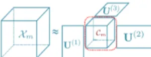
1) Tucker Decomposition: It represents a tensor Xm ∈
RI1×I2×···×IN as a core tensor with factor matrices [2]:
Xm= Cm×1U(1)×2U(2)· · · ×NU(N), (2)
where {U(n) ∈ RIn×Rn, n = 1,2· · ·N, and R
n < In}
are factor matrices with orthonormal columns and Cm ∈
RR1×R2×···×RN is the core tensor with lower dimension. The
Fig. 1. The Tucker decomposition of a third-order tensor sampleXm, where
the core tensorCmconsists of extracted features fromXm.
Fig. 2. The CP decomposition of a third-order tensor sampleXm, where the core tensorDmis super-diagonal and its elements{dm1, dm2,· · ·, dmR}
(i.e. feature vectordm) are viewed as extracted features fromXm.
Tucker-rank of an Nth-order tensor X is an N-dimensional vector, denoted as r = [R1,· · ·, Rn,· · ·, RN], whose n-th
entry Rn is the rank of the mode-n unfolded matrix X(mn)
of Xm. Figure 1 illustrates this decomposition. In this paper,
Tucker-rank is equivalent to the dimension of features (each core tensor). Based on Tucker decomposition, Liu et al.[25] have defined Tucker-based Tensor Nuclear Norm, that is,
Definition 3. Tucker-based Tensor Nuclear Norm [25] of a tensor X is defined as: kX k∗ = PNn=1kX(n)k∗ =
PN
n=1
PRn
j=1σj, whereX(n) is the mode-n unfolding matrix
ofX and σj is the singular values of the unfolded matrix.
2) CP Decomposition: It decomposes a tensor Xm ∈
RI1×···×IN as the sum of a set of weighted rank-one tensors:
Xm = R X r=1 dmru(1)r ◦u(2)r ◦ · · · ◦u(rN) = Dm×1U(1)×2U(2)· · · ×NU(N), (3)
where each common factor {u(rn), n = 1,· · · , N} is a
unit vector with a weight absorbed into the weight vector
d= [dm1,· · ·dmr,· · ·dmR]⊤ ∈RR, and ◦ denotes the outer
product [2]. Figure 2 shows that CP decomposition can also be reformulated as Tucker decomposition where the core tensor
Dm is super-diagonal, i.e., Dm(r,· · · , r) = dmr. R is the
CP-rankas the minimum number of rank-one components. In this paper, CP-rank is equivalent to the dimension of features (each weight vector). Based on orthogonal CP decomposition, we have defined the CP-based Tensor Nuclear Norm:
Definition 4. CP-based Tensor Nuclear Norm [32] of a tensor X is defined as the L1 norm of the weight vector d of its orthogonal CP decomposition:kX kCP=kdk1.
C. Related Work
Considering the target problem of extracting features from incomplete data, there are four categories of related ap-proaches, which are briefly summarized as follows.
1) Tensor Completion Approach: Tensor completion ap-proach is extended from the matrix case [23] and widely used for recovering missing data. There are many successful tensor completion methods, such as HaLRTC [25], TenALS [27], TNCP [26] and [35], [20], [36], [37]. These completion methods can yield good recovery results under typical condi-tions, but they focus only on estimating missing data instead of extracting informative features.
2) Feature Extraction Approach: Many tensor methods have been proposed for feature extraction directly from mul-tilinear data, e.g., the classical MPCA [3] and [4], [5], [6],
[38], [11], [39], [40], [41], [42]. These methods can achieve state-of-the-art results for learning features from complete (and noisy) tensors, however, they cannot perform well on data with missing values.
3) Supervised Classification Approach: Some classification algorithms have been well studied for classifying low-rank missing data [12], [16]. Besides, a few studies have integrated a discriminant analysis criterion into low-rank matrix/tensor completion models for classification [29], [30]. However, these methods require labels which are expensive and difficult to obtain in practice, especially for incomplete data.
4) Subspace Clustering Approach: Subspace clustering models such as sparse subspace clustering [43] were applied in the presence of missing data in [21], [22]. In addition, some studies have incorporated matrix completion approaches with subspace clustering for incomplete matrices [44], [45]. However, these algorithms do not yield good results for learning features from incomplete tensors because they are developed for clustering incomplete vectors/matrices.
In Sec. IV, we compare the proposed unsupervised methods with related state-of-the-art algorithms selected the abovemen-tioned category3) as they are supervised.
III. THEPROPOSED: TDVM-TUCKER ANDTDVM-CP
A. Problem Definition
Given a total M tensor samples {T1,· · ·,Tm,· · · ,TM}
withmissing entriesin each sampleTm∈RI1×···×IN.Inis the
mode-n dimension. We denote T = [T1,· · · ,Tm,· · · TM] ∈
RI1×···×IN×M, where theM are the number of tensor samples
concatenated along the mode-(N + 1) of T. To achieve feature extraction (dimension reduction) objective, we aim to directly extract low-dimensional features from the given high-dimensional incomplete tensors T.
Remark 1: This problem is different from the case of data with corruptions (e.g., noise and outliers), which has been well studied in [11], [46], [47], [43]. Missing data could be equivalent to the corruption case only if the corruptions are arbitrary and the indices of corruptions are known. However, in reality, the magnitudes of corruptions are not arbitrarily large. In other words, here we study a different feature extraction problem that existing methods cannot solve well.
To solve this problem, we propose an unsupervised feature extraction approach by incorporatinglow-rankTensor DecompositionwithfeatureVarianceMaximization(TDVM). Based on two widely used Tucker and CP decomposition models, we develop two algorithms of TDVM as follows.
B. TDVM-Tucker: Learning Low-dimensional Tensor Features
We first propose a TDVM method based on orthogonal Tucker decomposition: we impose the Tucker-based tensor nuclear norm on the core tensors while minimizing the re-construction error, and meanwhile maximize the variance of core tensors (features), i.e., incorporating low-rank Tucker
Decomposition with feature Variance Maximization, namely
TDVM-Tucker: min Xm,Cm,U(n) M X m=1 1 2kXm− Cm×1U (1)· · · × NU(N)k2F + M X m=1 kCmk∗ − M X m=1 1 2kCm−Ck¯ 2 F, s.t. PΩ(Xm) =PΩ(Tm),U(n) ⊤ U(n)=I, n= 1· · ·N, (4) where{U(n)∈RIn×Rn}N
n=1are common factor matrices with
orthonormal columns.I∈RRn×Rnis an identity matrix.C
m∈
RR1×···×RN is the core tensor, which consists of theextracted
featuresof an incomplete tensorTm with observed entries in
Ω.kCmk∗is the Tucker-based tensor nuclear norm ofCm.C¯=
1
M
PM
m=1Cmis the mean of core tensors (extracted features).
To optimize the objective function of TDVM-Tucker using ADMM, we apply the variable splitting technique, introduce a set ofauxiliary variables{Sm∈RR1×···×RN, m= 1· · ·M},
and then reformulate Eq. (4) as follows:
min Xm,Cm,Sm,U(n) M X m=1 1 2kXm− Cm×1U (1)· · · × NU(N)k2F + M X m=1 kSmk∗ − M X m=1 1 2kCm−Ck¯ 2 F, s.t. PΩ(Xm) =PΩ(Tm),Sm=Cm,U(n) ⊤ U(n)=I. (5)
Remark 2:The objective function Eq. (5) integrates three terms into a unified framework. The first and second term lead to low-rank Tucker approximation, which aims to minimize the reconstruction error and obtains low-dimensional features. Because imposing the Tucker-based tensor nuclear norm on a core tensor Cm is equivalent to that on its original tensor
Xm [48], we obtain a low-rank solution, i.e., Rn can be
small (Rn< In). Therefore, the feature subspace is naturally
low-dimensional. Moreover, imposing nuclear norm on core tensors instead of original ones reduces the computational cost. The third term (minimizing −PM
m=1 12kCm−Ck¯
2
F) aims to
maximize the variance of learned features inspired by PCA. TDVM-Tucker thus explores the relationship among tensor samples via feature variance maximization while estimating the missing data via low-rank Tucker approximation.
1) Derivation of TDVM-Tucker by ADMM: To facilitate the derivation of Eq. (5), we reformulate the equation by unfolding each tensor variable along mode-n and absorbing the constraints 1. Thus, we obtain the Lagrange function as follows: L = M X m=1 N X n=1 1 2kX (n) m −U(n)C(mn)H(n) ⊤ k2F + kS(mn)k∗ + hYmn,C(mn) − S(mn)i + µ 2kC (n) m −S(mn)k2F − 1 2kC (n) m −C¯(n)k2F (6) whereH(n)=U(N)N· · ·NU(n+1)NU(n−1)· · ·NU(1) ∈ RQj6=nIj×Qj6=nRj, and µ and {Y mn ∈ RRn× Q j6=nRj, n = 1,· · ·, N, m = 1,· · ·, M} are the Lagrange multipliers.
X(mn)∈RIn× Q j6=nIj and{C(n) m ,S(mn),C¯(n)} ∈RRn× Q j6=nRj
are the mode-n unfolded matrices of Xm and {core tensor
Cm, auxiliary variableSm, mean of featuresC}¯ , respectively.
ADMM solves the problem (6) by successively minimizing
L over{S(mn),U(n),Cm(n),X(mn)}, and then updatingYmn.
1For simplicity, the iteration number k is omitted in the updates of all
Algorithm 1Low-rankTensor (Tucker)Decomposition with FeatureVariance Maximization (TDVM-Tucker)
1: Input: Incomplete tensors PΩ(T), Ω, µ, and the maximum
iterations K, feature dimension D = [R1,· · ·, RN]
(Tucker-rank), and stopping tolerancetol.
2: Initialization: Set PΩ(Xm) =PΩ(Tm),PΩc(Xm) =0, m = 1,· · ·, M; initialize{Cm}Mm=1and {U(n)}Nn=1 randomly;ρ= 10, µmax= 1e10.
3: fork= 1toK do 4: form= 1toM do 5: forn= 1toN do
6: Update S(mn), U(n) and C(mn) by (8), (11) and (13)
respectively.
7: UpdateYmnbyYmn=Ymn+µ(C(mn)−S(mn)).
8: end for
9: UpdateXmby (15).
10: end for
11: IfkCm− Smk2F/kCmk2F <tol, break; otherwise, continue.
12: Updateµk+1= min(ρµk, µmax).
13: end for
14: Output: Tensorial features: C = [C1,· · ·,Cm,· · · CM] ∈ RR1×···×RN×M.
a) UpdateS(mn): Eq. (6) with respect to S(mn) is,
L S(mn)= M X m=1 N X n=1 kS(n) m k∗+ µ 2k(C (n) m +Ymn/µ)−S(mn)k 2 F , (7)
whereS(mn)is computed via soft-thresholding operator [49]:
S(mn)=prox1/µ(C (n) m +Ymn/µ) =Udiag(maxσ− 1 µ,0)V ⊤ , (8)
where prox is the soft-thresholding operation and
U diag(maxσ−µ1,0)V⊤ is the SVD of (C(mn)+Ymn/µ).
b) UpdateU(n): Eq. (6) with respect toU(n)is:
LU(n)= M X m=1 N X n=1 1 2kX (n) m −U (n)C(n) m H (n)⊤ k2F,s.t.U(n)⊤U(n)=I, (9)
The minimization of (9) over the matrices
{U(1),· · ·,U(N)}with orthonormal columns is equivalent to
the maximization of the following problem [50]:
U(n)= arg max trace U(n)⊤Xm(n)(C(mn)H(n)⊤)
⊤
(10) where trace() is the trace of a matrix, and we denoteW(n)=
C(mn)H(n)
⊤
. The problem (10) is actually the well-known orthogonal Procrustes problem [51], whose global optimal solution is given by the SVD ofX(mn)W(n)
⊤
, i.e.,
U(n)= ˆU(n)( ˆV(n))⊤, (11) where Uˆ(n) andVˆ(n) are the left and right singular vectors of SVD of X(mn)W(n)
⊤
, respectively.
c) Update C(mn) : Eq. (6) with respect to C(mn) is:
LC(mn) = M X m=1 N X n=1 kX(mn)−U(n)C(mn)H(n) ⊤ k2F + µ 2kC (n) m − S(mn) + Ymn/µk2F − 1 2k(1− 1 M)C (n) m − 1 M M X j6=m C(jn)k2F , (12)
setting the partial derivative ∂LC(mn)/∂C
(n) m to zero, we get: C(mn)= M2 M2µ+ 2M−1 µS(mn)−Ymn + U(n) ⊤ X(mn)H(n)− ( 1 M − 1 M2) M X j6=m C(jn) . (13)
d) UpdateXm: Eq. (5) with respect toXmis:
M X m=1 1 2kXm− Cm×1U (1)× 2U(2)· · · ×NU(N)k2F, s.t.PΩ(Xm) =PΩ(Tm), (14)
by deriving the Karush-Kuhn-Tucker (KKT) conditions for function (14), we can update Xm by:
Xm=PΩ(Xm) +PΩc(Cm×1U(1)×2U(2)· · · ×NU(N)). (15)
We summarize the proposed method, TDVM-Tucker, in
Algorithm 1.
Remark 3:TDVM-Tucker explores the relationship among tensor samples via feature variance maximization while esti-mating the missing data via low-rank Tucker approximation, leading to low-dimensional informative features directly from observed entries. The proposed methods differ from both tensor completion methods and two-step strategies as follows.
• Tensor completion methods aim to recover incomplete tensors only without exploring the relationship among samples for effective feature extraction. In contrast, TDVM-Tucker focuses on extracting low-dimensional features instead of estimating missing data. Moreover, TDVM utilizes a feature constraint (feature variance maximization) to capture the relationship among samples for extracting informative features.
• Unlike the “two-step” strategies, which learn the features
of incomplete data via two separate stages, TDVM-Tucker simultaneously estimates missing entries and learns low-dimensional features directly from the ob-served entries in the unified framework. The “two-step” strategies can amplify the approximation error because the missing data and the features are learned in separate stages, and the reconstruction error from the tensor com-pletion step can deteriorate the performance of feature extraction in the subsequent step. This claim has been ver-ified by our experimental results (as shown in the Tables I, II and III in Section IV-C). Therefore, TDVM-Tucker and TDVM-CP (which is introduced in the following) can extract more informative features within the unified framework.
C. TDVM-CP: Learning Low-dimensional Vector Features
We further propose another new TDVM method to learn low-dimensional vectorial features based on CP decomposition, i.e., incorporating low-rank CP decomposition with feature variance maximization, namely TDVM-CP. Be-cause tensor decomposition with missing data is more chal-lenging than that with complete data in traditional problems, here we consider incorporating orthogonality into the CP model for TDVM-CP (i.e., imposing orthogonality constraints on factors{u(rn)} in Eq. (3)) with the following two
motiva-tions:
• Like HOSVD [31], CP decomposition can be regarded as a generalization of SVD to tensors [52]. It appears natural to inherit the orthogonality of SVD in the CP model.
• The orthogonality constraint is considered unnecessary in general or even impossible in certain cases in exact CP decomposition [53], [54], [55], but some studies have
proved that imposing orthogonality in CP decomposition can transform a non-unique tensor model into a unique one with guaranteed optimality [54], [27], [56].
Like the orthogonality used in TDVM-Tucker, we believe that imposing orthogonality constraints can help TDVM-CP estimate missing values and extract features better. In addition, here we do not use the Tucker-based nuclear norm [25]; instead, we use a new CP-based tensor nuclear norm2 [32] to achieve low-rank CP approximation.
In other words, TDVM-CP couples orthogonal CP decomposition with the CP-based tensor nuclear norm for the low-rank approximation, while maximizing the variance of learned features as the feature regularization term. Thus, the objective function of TDVM-CP is as follows:
min Xm,dm,u(rn),R M X m=1 1 2kXm− R X r=1 dmru(1)r ◦ · · · ◦u(rN)k2F + M X m=1 λkdmk1− M X m=1 1 2kdm−¯dk 2 2, s.t.PΩ(Xm) =PΩ(Tm),u(rn) ⊤ u(rn)= 1, n= 1· · ·N, u(rn) ⊤ u(qn)= 0, q= 1· · ·r−1, r= 1· · ·R, (16)
where kdmk1 is the CP-based tensor nuclear norm on each
weight vector, and we view the weight vector dm ∈ RR of
the orthogonal CP decomposition (analogous to the vector of singular values of a matrix) as the feature vector extracted from a tensor sample Xm.d¯ = M1 PMm=1dm is the mean of
the weight vectors (extracted features). λ > 0 is a penalty parameter. Compared with TDVM-Tucker, TDVM-CP can obtain much lower dimensional features because it learns vectorial features from each tensor sample.
1) ADMM-BCD Joint Optimization for TDVM-CP: To solve the objective function Eq. (16) which is non-convex and non-smooth, we design a ADMM-BCD joint optimization scheme. We divide all the target variables into M ×(R+ 1)
groups:{{dmr,u(1)r ,u(2)r ,· · · ,ur(N)}Rr=1,Xm}Mm=1, where we
optimize a group of variables while fixing the other groups, and update one variable while fixing the other variables in each group. After updating the R+ 1 groups for each sample using BCD, we jump to the outside loop to update all samples iteratively using ADMM. To apply ADMM, we introduce a set of auxiliary variables {sm∈RR}Mm=1 for the weight vectors {dm}Mm=1, i.e., sm = dm ∈ RR, m = 1· · ·M. Then, we
formulate the Lagrangian function of Eq. (16) as follows:
L = M X m=1 1 2kXm− R X r=1 dmru(1)r ◦ · · · ◦ur(N)k2F+λkdmk1 − 1 2ksm−¯sk 2 2+hym,dm−smi+γ 2kdm−smk 2 2 − η(u(rn) ⊤ u(rn)−1) − r−1 X q=1 µqu(rn) ⊤ u(qn), (17)
whereγ, η,{µq}rq−=11 andymare the Lagrange multipliers.
In the ADMM-BCD joint optimization, we first update the variables{dmr,u(1)r ,u(2)r ,· · · ,u(rN)}Rr=1 of each data sample via BCD. Thus, we formulate the Eq. (17) with respect to the r-th group{dmr,u(1)r ,u(2)r · · ·,u(rN)} as follows:
2For easy reading, we usekd
mk1 instead ofkXmkCPin the derivation.
Ld mr,u(rn) = 1 2kXmr−dmru (1) r ◦u(2)r ◦ · · · ◦ur(N)k2F+λ|dmr| + γ 2kdmr+ymr/γ−smrk 2 2 − η(u(rn) ⊤ u(rn)−1)− r−1 X q=1 µqu(rn) ⊤ u(qn), (18) whereXmr=Xm−Prq−=11dmqu(1)q ◦u(2)q ◦ · · · ◦u(qN) is the
residual of the approximation of each tensor sample.
a) Updateu(rn): Eq. (18) with respect tou(rn) is,
Lu(n) r = 1 2kXmr−dmru (n) r ◦u(2)r · · · ◦u(rN)k2F − η(u(rn) ⊤ u(rn)−1)− r−1 X q=1 µqu(rn)u(qn). (19)
Then we set the partial derivative of Lu(rn) with respect to
u(rn)to zero and eliminate the Lagrange multipliers, and get:
u(rn)=(Xmr×j{u(rj)}j6=n)/dmr − r−1 X q=1 u(qn) ⊤ (Xmr×j{ur(j)}j6=n) u(qn) /dmr, (20) where Xmr ×j {u(rj)}j=6 n = Xmr ×1 u(1)r · · · ×(n−1) u(rn−1)×(n+1)u(rn+1)· · · ×N u(rN), j = 1,2,· · ·, n−1, n+ 1,· · ·, N, and we normalizeu(rn)=ur(n)/ku(rn)k2. Note that
we only update the variable groups with non-zero weights (i.e. dmr6= 0).
b) Updatedmr: Eq. (18) with respect todmr is:
Ldmr = 1 2kXr−dmru (1) r ◦u(2)r · · · ◦ur(n)k2F + λ|dmr| +γ 2kdmr+ymr/γ−smrk 2 2. (21)
Setting the partial derivative∂Ldmr/∂dmr to zero, we obtain,
dmr= 1 (1 +γ) γsmr−ymr+Xr×1u(1)r ×2u(2)r · · · ×Nu(rN)−λ|dmr|/∂dmr . (22)
According to the soft thresholding algorithm [57] for L1
regularization, we updatedmr by:
dmr=shrinkt(Q) = Q−t (Q > t) 0 (|Q| ≤t) Q+t (Q <−t) . (23)
where shrink is the shrinkage operator [57], and t = λ
(1+γ), Q= 1
(1+γ)(γsmr−ymr+Xr×1u(1)r ×2· · · ×Nu(rN)).
After updating{dmr,u(1)r ,u(2)r ,· · ·,u(rN)}Rr=1by the BCD
method, we jump out of the inner loop for each tensor sample and update the variables{sm,Xm}Mm=1for all tensor samples
iterativelyvia ADMM.
c) Updatesm: Eq. (17) with respect tosmis,
Lsm = M X m=1 1 2γkdm+ym/γ−smk 2 2− M X m=1 1 2ksm−¯sk 2 2, (24)
whereym consists of Lagrange multipliers. Then we set the
partial derivative∂Lsm/∂sm to zero and obtain,
sm= M 2 γM2+ 1−2M+M2 γdm+ym + M−1 γM2+ 1−2M+M2 M X j6=m sj (25)
Algorithm 2 Low-rank Tensor (CP) Decomposition with FeatureVariance Maximization (TDVM-CP)
1: Input:Incomplete tensorsPΩ(T),Ω,λ, feature dimensionD=
R (CP-rank), maximum iterationsK, andtol.
2: Initialization: Set PΩ(Xm) = PΩ(Tm), PΩc(Xm) = 0, γ = 10; Initialize{u(1)r ,u(2)r ,· · ·ur(N)}Rr=1,{dm}Mm=1 randomly. 3: fork= 1, ..., Kdo 4: form= 1, ..., M do 5: Xmr =Xm; 6: forr= 1, ..., Rdo 7: ifdmr6= 0then
8: Updateu(rn)and dmr by (20) and (23),respectively.
9: Xmr=Xmr−dmrur(1)◦u(2)r · · · ◦u(rN).
10: end if 11: end for
12: UpdatesmandXm by (24) and (27) respectively.
13: Updateym=ym+γ(dm−sm)
14: end for
15: Ifkdm−smk22/kdmk22<tol, break; otherwise, continue.
16: end for
17: output:Vectorial featuresD= [d1,· · ·dm,· · ·dM]∈RR×M. d) UpdateXm: Eq. (16) with respect toXmis,
min Xm 1 2kXm− R X r=1 dmru(1)r ◦u(2)r · · · ◦u(rN)k2F, s.t.PΩ(Xm) =PΩ(Tm), (26)
by deriving KKT conditions for Eq. (26), Xm is updated by:
Xm=PΩ(Xm) +PΩc( R
X
r=1
dmru(1)r ◦u(2)r · · · ◦u(rN)). (27)
Using the ADMM-BCD joint optimization, we solve each subproblem of Eq. (16) in a closed-form. Finally, we summa-rize the proposed TDVM-CP inAlgorithm 2.
Remark 4: TDVM-CPis similar in spirit to TDVM-Tucker, but it can yields features with lower dimension than TDVM-Tucker: the former extracts low-dimensional vector features from each data sample, while the latter aims to learn low-dimensional tensor features from each sample. Thus, using TDVM-CP to extract features can reduce the computational cost and memory requirements for further applications such as classification and clustering.
D. Computational Complexity Analysis
For TDVM-Tucker, we set the feature dimensions (Tucker-rank) R1 = R2· · · =RN =R for simplicity. In each
itera-tion, the time complexity of computing the soft-thresholding operator (8) is O(M N RN+1). The time complexities of
multiplications in (11)/(13) and (15) are O(M N R(QN
j=1Ij))
and O(M R(QN
j=1Ij)), respectively. Thus, the total time
complexity of TDVM-Tucker is O(M(N + 1)R(QN
j=1Ij))
in each iteration. For TDVM-CP, the time complexity of performing the shrinkage operator in (23) is O(R(QN
j=1Ij).
This is also the time complexity of computing{u(rn)}Nn=1and
Eq. (27). Hence, the total time complexity of TDVM-CP is O(M R(QN
j=1Ij)in each iteration.
E. Discussion: General Model–TDFR
The proposed TDVM-Tucker and TDVM-CP essentially can be summarized into a general model, i.e., low-rank Tensor
Decomposition with FeatureRegularization (TDFR):
min
X,ZF(X, Z) +G(Z)s.t.PΩ(X) =PΩ(T), (28)
where F(X, Z) refers to a low-rank tensor decomposition model and G(Z) is a regularization of target features Z.
X ∈RI1×I2×···IN×M is the approximation of incomplete data
(tensors) T based on observed entries indexed by Ω. Z is a component of X and could be a lower-dimensional tensor (e.g., a core tensor of Tucker model) or vector (e.g., a weight vector of CP model) that consists of all features extracted from
T.
In this paper, we specify TDFR by TDVM-Tucker and TDVM-CP. In addition, we briefly discuss more specific cases of TDFR. For example, considering the whole dataset as a tensor including all samples along the last mode, we can specify TDFR as follows: min X,C,U(n),Z 1 2kX −C×1U (1)× 2U(2)· · · ×NU(N)×N+1Zk2F + kCk∗ − 1 2kZ ⊤ k2F, s.t. PΩ(X) =PΩ(T),U(n) ⊤ U(n)=I, n= 1· · ·N, (29)
where the(N+1)th factor matrixZ∈RM×R(N+1) are viewed as the extracted features from T = [T1,· · ·,Tm,· · · TM] ∈
RI1×···×IN×M. Such usage of treating the (N + 1)th factor
matrix as features can also be found in [58], [59]. Inspired by PCA, the third term:min−12kZ⊤k2
F = maxtrace(ZZ⊤), aims
to maximize the variance of extracted features. Due to space limitations, more specific cases are discussed in Appendix A of the Supplementary Material3.
Remark 5: As TDFR simultaneously estimates missing data via low-rank tensor approximation and explores the relationship among samples via feature regularization (e.g., maximizing variance of features in TDVM), we assume that TDFR can solve the problem of extracting features from incomplete tensors. In addition to the two proposed methods, there are many variants of specific cases of the general model TDFR: 1) For the low-rank approximation F(X, Z) of Eq. (28), we can not only use Tucker and CP decompositions in conjunction with the Tucker- and CP-based tensor nuclear norm, but can also consider other tensor decomposition models such as Tensor SVD [60], [11], Tensor-train decomposition [61], [62], etc., coupled with other constraints such as tensor nuclear norm [60], [11] to achieve low-rank tensor approxi-mation; 2) For the feature regularization term G(Z), we can use not only variance maximization for regularization such as TDVM but also other constraints such as uncorrelation or orthogonality, etc., to learn informative features.
IV. EXPERIMENTS
We evaluate the performance of the proposed TDVM-Tucker and TDVM-CP on six real-world tensor datasets with 30%−90% missing entries under multi-block missing settings. “MR” refers to the Missing Ratio. We implement the proposed methods in MATLAB, and all experiments are performed on a PC (Intel Xeon(R) 4.0 GHz, 64 GB memory).
3Supplementary Material: https://www.dropbox.com/sh/
A. Experimental Setup
1) Data: We evaluate TDVM-Tucker and TDVM-CP on
six real-world datasets for three applications, including four third-order tensors and two fourth-order tensors 4:
• For face recognition, we use two face datasets: one is
a subset of the Facial Recognition Technology database (FERET)5 [63], which has 721 face samples from 70 subjects. Each subject has 8 to 31 face images with at most 15 degrees of pose variation, and each face image is normalized to an80×60gray image. The other dataset is a subset of the extended Yale Face Database B (YaleB)6 [64], which has 2414 face samples from 38 subjects. Each subject has 59 to 64 near frontal images under different illumination and each image is normalized to a32×32
gray image.
• For object/action classification tasks, we evaluate two
datasets: one is a subset of theCOIL-100image database, which contains 100 different objects, each viewed from 72 different angles7[65]. The size of each sample (totally 1000 samples) is normalized to a 64×64 gray image following [66]. The other dataset is a subset of the
Weizmann action dataset 8 [67], which consists of 80 videos of 8 actors performing ten different actions: “bend-ing”, “jump“bend-ing”, “jumping jacks”, “jumping in place”, “running”, “galloping sideways”, “skipping”, “walking, “one hand-waving”, and “two hands waving”. Each video is resized to 32×22×10.
• Forface/gait clusteringtests, we also test two datasets: one is a subset of the AR face database [68], which contains 1200 face images with size 55 ×40 of 100 subjects including images of non-occluded faces, and face occluded by scarves/glasses following [66]9; the other dataset is the gallery set (731 samples from 71 subjects) of theUSFHumanID “GaitChallenge” database10[69]. Each gait video sample is resized to 64×44×20.
2) Compared Methods: We compare TDVM-Tucker and TDVM-CP with 17 methods in four categories11:
(i) Three Tucker-/CP- based tensor completion methods:
HaLRTC [25],TenALS[27] andTNCP[26].
(ii) Nine {tensor completion methods + feature extraction methods}(i.e., “two-step” strategies):HaLRTC+MPCA
[3], TenALS + MPCA, TNCP + MPCA, HaLRTC +
SOMPCARS [6], TenALS + SOMPCARS, TNCP +
4For fast evaluation, we use resized tensor samples with smaller dimensions,
while the proposed methods are applicable to original (larger) tensors without subsampling (resizing). Refer to Appendix D of the Supplementary Material for results on large tensors.
5http://www.dsp.utoronto.ca/∼haiping/MSL.html 6http://www.cad.zju.edu.cn/home/dengcai/Data/FaceData.html 7http://machineilab.org/users/pengxi 8http://www.wisdom.weizmann.ac.il/∼vision/SpaceTimeActions.html 9http://machineilab.org/users/pengxi 10http://www.dsp.utoronto.ca/∼haiping/MSL.html
11We have also compared with the state-of-the-art tensor singular value decomposition
(t-SVD) methods such as [70] and its combined two-step strategies. Although the t-SVD based tensor completion methods slightly outperform the Tucker and CP based methods (such as HaLRTC and TNCP), they still give much poorer feature extraction results than our TDVM methods. Because the proposed methods are based on the Tucker and CP models, we do not present the comparison against t-SVD methods here for simplicity and please refer to Appendix C of the Supplementary Material for these results.
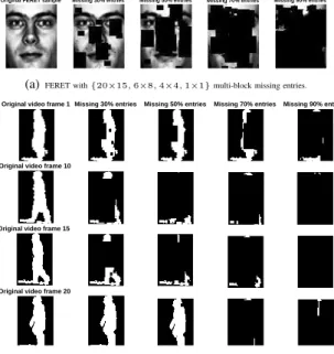
Original FERET sample Missing 30% entries Missing 50% entries Missing 70% entries Missing 90% entries
(a)FERET with{20×15,6×8,4×4,1×1}multi-block missing entries.
Original video frame 1 Missing 30% entries Missing 50% entries Missing 70% entries Missing 90% entries
Original video frame 10
Original video frame 15
Original video frame 20
(b)USF gait with{32×20×10,20×15×5,4×3×4,1×1×1}multi-block missing entries.
Fig. 3. Examples of (a) one sample of FERET database (b) four frames of the first video sample (20 frames) of USF gait database, with
{30%,50%,70%,90%}missing entries generated by MbM settings.
SOMPCARS, HaLRTC + LRANTD [4], TenALS +
LRANTD,TNCP +LRANTD.
(iii) Onerobust tensor feature learning method:TRPCA[11]. (iv) Four clustering methods (used for the comparison of clustering with missing data): Sparse subspace clustering (SSC) [43], Zero-Fill + SSC (ZF + SSC) [21], SSC by Column-wise Expectation-based Completion (SSC-CEC) [21], Sparse Representation with Missing Entries and Matrix Completion (SRME-MC) [22].
We compare the 13 methods of the first three categories with respect to face recognition and object/action classification tasks, and compare all 17 methods in face/gait clustering tests. After feature extraction, we use the Nearest Neighbors Classifier (NNC) to evaluate the extracted features for face recognition and object/action classification. For face/gait clus-tering tests, we use the K-means [71] to cluster the features extracted by the first 13 methods and use a spectral clustering technique as a post-processing step for the four subspace clustering methods.
3) Multi-block Missing (MbM) Setting: In this paper, we design a“Multi-block Missing (MbM)” setting to generate random missing patterns of tensors. According to the data sample size, we use a set of tensorial blocks with different sizes as missing blocks to generate missing entries randomly in each tensor sample. We progress from the largest missing blocks to the smallest missing blocks to generate missing patterns until the required ratio of missing entries is achieved. For example, we can use a random set of missing blocks
{32×20×10,20×15×5,4×3×4,1×1×1} to obtain an incomplete USF gait database (sample size64×44×20) with
50% missing entries. We first use thek largest (32×20×10) blocks to create missing entries randomly until the(k+ 1)th largest block exceeds the required missing ratio (e.g.,k= 5); then we use thepsecond largest (20×15×5) blocks until the
(p+ 1)th second largest block exceeds the required missing ratio (e.g., p= 12). We continue by using the sthird largest
(4×3×4) blocks (e.g.,s = 25) to generate the missing data successively. Finally, we use the q smallest missing blocks with smallest size (e.g., q = 70) to make up the remaining missing region. Thus, we use(k+p+s+q)missing blocks of different sizes to generate an incomplete USF gait tensor sample with 50%missing entries. Here, these missing blocks can be overlapped (i.e., the values of k, p, s, q are different in different samples) and the missing blocks are distributed randomly in each tensor sample. Hence, the irregular missing shapes (positions of missing data, i.e., Ω) are different in each tensor sample, while the total number of missing entries is the same. Nevertheless, one can set any types of MbM sets with multiple blocks of different sizes under the MbM setting. Figure 3 illustrates the data samples with missing entries generated by the proposed MbM setting.
Remark 6: The Multi-block Missing setting generates different irregular missing shapes (missing patterns) in tensor samples, which is more general and practical in real-world applications. MbM setting with only one type of block (with size = 1) is equivalent to the pixel-based missing (uniformly selecting MR (e.g., MR = 50%) pixels (entries) from each tensor sample as missing at random) which is widely used in matrix/tensor completion fields. MbM setting with only one type of block (with size>1) is equivalent to the block-based missing setting (randomly selecting a single block entries of each tensor sample as missing) which is also commonly used in missing data imputation. In other words, existing missing data settings are special cases of our MbM setting. Intuitively, handling data with generalmulti-block missingis more difficult than that with pixel-based missingandblock-based missingif the number of missing entries is the same. The reason is that the MbM setting is somehow close to thenon-random missing
setting especially when MR is higher (e.g., when MR= 90%, some whole rows/columns of images/videos are missing as shown in Figure 3), although the MbM setting is essentially random block missing with overlapping.
4) Parameter Settings: We set the maximum iterationsK= 500,tol= 1e−5for all methods, although our methods usually converge within10iterations. For Tucker decomposition-based methods, namely, TDVM-Tucker and LRANTD, we set the feature dimension D = [R1, R2,· · ·, RN] (Tucker-rank) =
round(1/2×([I1, I2,· · ·IN]))for each tensor sample. For CP
decomposition-based methods, namely, TDVM-CP, TenALS and TNCP, we set D=R (CP-rank) = round (min{1/2×
mean([I1, I2,· · ·, IN]),min([I1, I2,· · ·, IN])})for each
sam-ple. For other parameters of the compared methods, we have tuned the parameters based on the original papers to obtain the best results under same experimental settings. On the other hand, we further evaluate extracted features for classification via NNC, in which we randomly select L={1,7}extracted feature samples from each subject of FERET for training in NNC. Similarly, we setL={5,50},{1,8}and{1,7}on the YaleB, COIL-100 and Weizmann datasets, respectively.
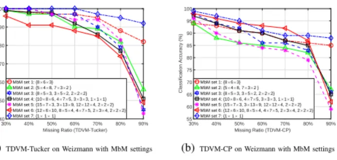
B. Analysis of Different (Parameter) Settings and Convergence 1) Effect of Different Multi-block Missing Settings: Here, we study the effect of applying Tucker and TDVM-CP to datasets with different MbM settings. We randomly set
30% 40% 50% 60% 70% 80% 90% Missing Ratio (TDVM-Tucker) 40 50 60 70 80 90 100 Classification Accuracy (%) MbM set 1: {8×6×3} MbM set 2: {5×4×8, 7×3×2 } MbM set 3: {8×5×3, 3×5×2, 2×2×2} MbM set 4: {10×8×6, 4×7×5, 3×3×3, 1×1×1} MbM set 5: {15×7×3, 3×13×9, 12×12×4, 2×2×2} MbM set 6: {12×6×10, 8×5×4, 4×7×5, 2×3×4, 2×2×2} MbM set 7: {1× 1× 1}
(a)TDVM-Tucker on Weizmann with MbM settings
30% 40% 50% 60% 70% 80% 90% Missing Ratio (TDVM-CP) 55 60 65 70 75 80 85 90 95 100 Classification Accuracy (%) MbM set 1: {8×6×3} MbM set 2: {5×4×8, 7×3×2 } MbM set 3: {8×5×3, 3×5×2, 2×2×2} MbM set 4: {10×8×6, 4×7×5, 3×3×3, 1×1×1} MbM set 5: {15×7×3, 3×13×9, 12×12×4, 2×2×2} MbM set 6: {12×6×10, 8×5×4, 4×7×5, 2×3×4, 2×2×2} MbM set 7: {1× 1× 1}
(b)TDVM-CP on Weizmann with MbM settings
Fig. 4. Classification results of Weizmann with30%−90%missing entries generated by seven different MbM settings via TDVM-Tucker and TDVM-CP (feature dimensionD={16×11×5,10}respectively).
30% 40% 50% 60% 70% 80% 90% Missing Ratio (TDVM-Tucker) 20 40 60 80 100 Classification Accuracy (%) D1 = 30 × 30 ×30 D2 = 32 × 22 × 10 D3 = 25 × 20 × 10 D4 = 16 × 11 × 5 D5 = 8 × 6 × 3 D6 = 5 × 5 × 5 D7 = 2 × 2 × 2
(a)TDVM-Tucker with different feature dimensions
30% 40% 50% 60% 70% 80% 90% Missing Ratio (TDVM-CP) 40 50 60 70 80 90 100 Classification Accuracy (%) D1 = 32 D2 = 21 D3 = 15 D4 = 10 D5 = 8 D6 = 5 D7 = 3
(b)TDVM-CP with different feature dimensions
Fig. 5. Classification results on Weizmann with30%−90%missing entries (MbM set ={10×8×6,4×7×5,3×3×3,1×1×1}) via TDVM-Tucker and TDVM-CP with seven different feature dimensions.
seven MbM sets using different types of missing blocks to generate missing pattern on the Weizmann database to obtain incomplete Weizmann data, i.e., MbM set 1 using only one type of block with size {8×6×3}, which also refers to the commonly used block-based missing setting;MbM set 2using two types of blocks:{5×4×8,7×3×2};MbM set 3using three types of blocks:{8×5×3,3×5×2,2×2×2};MbM set 4using four types of blocks:{10×8×6,4×7×5,3×3×3,1×1×1};
MbM set 5 using four types of blocks: {15×7×3,3×13×
9,12×12×4,2×2×2};MbM set 6 using five types of blocks:
{12×6×10,8×5×4,4×7×5,2×3×4,2×2×2}; andMbM set 7
using only one type of block with size= 1(1×1×1), which is equivalent to the pixel-based missing setting widely used in matrix/tensor completion. Using the seven MbM sets, we generate an incomplete Weizmann database (32×22×10×80) with30%−90% missing entries. Tucker and TDVM-CP directly extract16×11×5×80and10×80features from these incomplete tensors, respectively, and these features are further evaluated via NNC usingL= 7video feature samples per subject (each subject has 8 samples) as training.
Figure 4 shows that on the Weizmann dataset with various missing patterns using different random MbM sets, both TDVM-Tucker and TDVM-CP consistently yield good results. Two cases are particularly worth mentioning. On the Weiz-mann dataset with MbM set 1 andset 7, TDVM-Tucker and TDVM-CP can achieve better classification results than other cases (MbM set 2-6) especially when MR>70%. This verifies our claim mentioned in Remark 6: handling data with the MbM setting which uses multiple missing blocks (MbM set 2-6) is more difficult than that with existing block-based missing (MbM set 1) and pixel-based missing (MbM set 7) settings. For general MbM settings (MbM set 2-6), TDVM-Tucker and TDVM-CP can obtain similar results with acceptable deviation of classification accuracy. On the other hand, using these
1 2 3 4 5 6 7 L (Training Sample Per Subject) 0.3 0.4 0.5 0.6 0.7 0.8 0.9 1 Classification Accuarcy (%) = 1 = 5 = 10 = 15 = 20 = 25 = 30 = 35 = 40 = 45 = 50
(a)TDVM-Tucker with differentµ
1 2 3 4 5 6 7 L (Training Sample Per Subject) 0.1 0.2 0.3 0.4 0.5 0.6 0.7 0.8 0.9 1 Classification Accuarcy (%) = 1 = 5 = 10 = 15 = 20 = 25 = 30 = 35 = 40 = 45 = 50 (b)TDVM-CP with differentλ
Fig. 6. Classification results on Weizmann with50%missing entries (MbM set ={10×8×6,4×7×5,3×3×3,1×1×1}) via TDVM-Tucker and TDVM-CP with 11 different values ofµandλ, respectively.
1 5 9 13 17 21 25 29 33 37 41 45 49 Number of Interations 10-15 10-10 10-5 100 Relative Error TDVM-Tucker (a)TDVM-Tucker 1 5 9 13 17 21 25 29 33 37 41 45 49 Number of Interations 10-10 10-5 100 Relative Error TDVM-CP (b)TDVM-CP
Fig. 7. Convergence curves of TDVM-Tucker and TDVM-CP in terms of Relative Error: kGm − Smk2F/kGmk2F and kdm −smk22/kdmk22
respectively, on Weizmann with 50% missing entries (MbM set ={10×
8×6,4×7×5,3×3×3,1×1×1}).
MbM sets with different types of missing blocks, the achieved missing ratios are likely slightly different, especially for these MbM sets without size = 1 block to make up the remaining missing entries. For example, with MbM set 5, we actually obtain Weizmann with 29.94% – 89.92% instead of exact
30%–90%missing entries because of the sizes of the missing blocks. This slight difference of actual number of missing entries can also slightly affect the classification results, leading to an increase in the deviation of classification accuracy under different MbM settings.
In short, the proposed TDVM-Tucker and TDVM-CP are are not highly sensitive to the missing patterns overall and consistently yield good results under various MbM settings. Thus, in the following tests, we test datasets with four types of missing blocks in MbM settings for simplicity, and each MbM set includes the size = 1block to ensure the total number of missing entries is the same under different MbM settings.
2) Effect of Different Feature Dimensions: We study the effect of different feature dimensions used in TDVM-Tucker and TDVM-CP for feature extraction on an incomplete Weiz-mann database. Figure 5 shows that, with different dimensions of features, TDVM-Tucker and TDVM-CP yield similar clas-sification results stably on the whole, except in the case of TDVM-Tucker with D7 = 2×2×2 (i.e., only 8 features are extracted from each 32×22×10 video) where the number of features is too limited to achieve good results. TDVM-CP obtains much fewer learned features, but it consistently achieve good results. On the other hand, as Tucker and TDVM-CP are based on the orthogonal Tucker and TDVM-CP models respec-tively, the dimension of effective features for TDVM-Tucker is upper-bound by the data dimension in each mode, and that of TDVM-CP is limited by the minimum sample dimension. Thus, setting {D1 = 30×30×30>32×22×10} for
TDVM-Tucker and {D1=32, D2=21, D3=15>10=min [32,22,10]}
for TDVM-CP leads to a slight deterioration of classification performance especially in the cases of Weizmann with higher missing ratio (e.g., MR= 90%), as seen from Figs. 5(a) and 5(b) respectively.
In short, the proposed methods are not sensitive to the feature dimensions. Since a larger feature dimension will lead to higher computational costs and memory requirements, and we aim to learn low-dimensional features, we thus set D=round(1/2×([I1, I2,· · ·IN]))andD=round(min{1/2×
mean([I1, I2,· · · , IN]),min([I1, I2,· · · , IN])}) for
TDVM-Tucker and TDVM-CP by default, respectively.
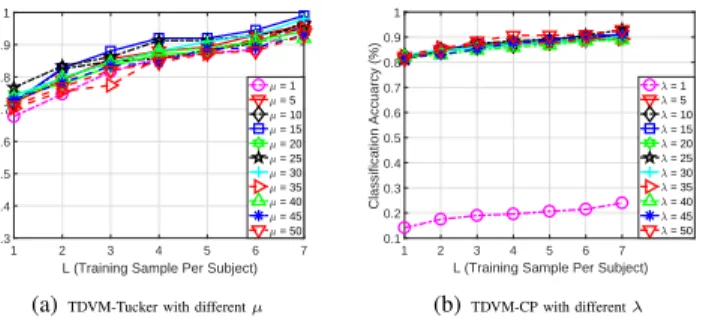
3) Sensitivity Analysis of Parameter µ and λ: Figure 6 shows the classification results given features extracted by TDVM-Tucker and TDVM-CP with 11 different values for the penalty parametersµandλ, respectively, on Weizmann videos with50% missing entries via an MbM set. Figure 6(a) show that TDVM-Tucker yields good results stably with different values of µ. Figure 6(b) shows that the feature extraction performance of TDVM-CP is also stable and not sensitive to the values of λ, except for the case in which λ = 1. In other words, the proposed methods are not sensitive to the parameters overall. In addition, as the parametersρandγcan be fixed (fixρ= 10,γ= 1) within Algorithm 1 and Algorithm 2 respectively based on preliminary studies, we thus do not examine them here.
In short, we do not need to carefully tune the parametersµ andλfor TDVM-Tucker and TDVM-CP, respectively. In this paper, we fixµ=λ= 10for all tests.
4) Convergence: We study the convergence of TDVM in terms of the relative error on a Weizmann dataset with
50% missing entries via an MbM set. Figure 7 shows that: Tucker converges within 10 iterations while TDVM-CP requires more iterations (about 20) to reach convergence. If settol= 1e−5, our methods converge fast with around 5-10 iterations.
C. Evaluation of Extracted Features from Incomplete Tensors
To save space, we report the results of six real tensor datasets with {30%,50%,70%,90%} missing pixels under random MbM settings in Tables I, II and III 12. We highlight the best results in bold font and underline the second best results, and we use “–” to indicate that the method diverges (e.g., TenALS) in some cases. The average results of 10 runs are reported.
1) Face Recognition: Table I shows that TDVM-Tucker and TDVM-CP consistently outperform all the methods com-pared in all cases. Specifically, TDVM-Tucker and TDVM-CP directly learn 40×30×721 features and 35×721 features from FERET (80×60×721) with {30%,50%,70%,90%}
missing pixels via a random MbM set ({32×32,10×4,8×
16,1×1}). As shown in the left half of Table I, TDVM-Tucker and TDVM-CP share the two best recognition results,
12The proposed methods are based on low-rank decompositions and thus
can yield good results on tensors with good low-rank structure even when the missing ratio reaches90%. However, if too many (e.g.,95%,99%) entries are missing, the performance of our methods will drop dramatically.
TABLE I
FACE RECOGNITION RESULTS(AVERAGE RECOGNITION RATES%)ON THEFERETANDYALEBDATABASE WITH{30%,50%,70%,90%}MISSING ENTRIES UNDERMULTI-BLOCKMISSINGSETTINGS.
Data FERET (Image sample size80×60) YaleB (Image sample size32×32) Multi-Block Missing Setting {20×15,6×8,4×4,1×1} {16×16,10×5, 4×8, 1×1}
Missing Ratio (MR) 30% 50% 70% 90% 30% 50% 70% 90% L 1 7 1 7 1 7 1 7 5 50 5 50 5 50 5 50 HaLRTC[25] 34.1 71.2 31.1 67.1 26.3 58.4 19.2 46.3 32.9 73.9 30.8 70.8 27.2 63.0 19.5 44.8 TenALS[27] 31.3 65.6 29.4 63.3 25.0 55.5 12.4 24.8 25.0 56.5 18.0 38.5 7.7 14.8 2.7 2.7 TNCP[26] 33.6 71.0 32.0 66.6 26.5 59.4 20.8 45.2 28.9 66.9 24.5 58.7 20.1 47.8 17.8 36.5 HaLRTC +MPCA[3] 40.4 73.8 30.8 65.2 21.2 51.7 16.9 41.0 24.7 65.6 12.9 38.4 10.2 18.5 8.7 20.7 TenALS +MPCA[3] 31.1 62.0 23.9 49.4 12.9 24.9 4.8 9.1 18.6 40.8 16.8 36.0 13.4 24.2 8.5 13.8 TNCP +MPCA[3] 33.4 63.7 19.7 33.7 13.7 22.3 12.6 18.4 19.9 55.4 11.4 30.7 12.9 26.3 10.3 16.1 HaLRTC +SOMPCARS[6] 32.0 63.7 25.7 51.1 17.7 30.8 12.2 19.6 11.6 23.3 11.4 20.1 11.2 19.3 8.5 11.7 TenALS +SOMPCARS[6] 28.5 52.2 11.8 17.1 6.4 7.8 3.6 4.9 11.1 24.0 12.9 22.4 11.1 20.8 8.4 14.4 TNCP +SOMPCARS[6] 29.5 55.2 14.4 26.4 7.5 10.7 8.5 10.0 17.8 38.8 15.3 33.7 9.8 17.7 6.2 10.3 HaLRTC +LRANTD[4] 34.0 72.3 30.5 66.4 25.3 58.3 19.2 45.7 24.5 58.4 21.4 52.3 17.6 42.5 13.8 29.7 TenALS +LRANTD[4] 30.9 65.5 29.0 63.2 26.4 58.4 14.6 29.4 12.7 27.5 12.9 26.5 13.2 25.6 9.5 16.5 TNCP +LRANTD[4] 34.1 71.0 31.1 67.9 26.8 60.2 20.1 45.0 21.1 49.6 17.8 41.9 16.3 36.6 15.5 31.2 TRPCA[11] 30.0 64.4 21.8 51.1 17.8 43.1 16.5 36.0 32.5 72.5 30.0 66.3 26.2 54.4 19.6 36.0 TDVM-Tucker 75.7 92.1 73.9 91.1 71.8 91.0 70.6 90.3 58.2 94.8 47.2 93.0 46.2 92.1 45.1 91.0 TDVM-CP 76.3 90.9 75.9 88.0 75.2 87.2 72.6 86.6 94.9 97.6 93.0 95.6 90.6 95.4 81.9 91.4 TABLE II
CLASSIFICATION RESULTS(AVERAGE CLASSIFICATION ACCURACIES%)OF THECOIL-100OBJECT IMAGES ANDWEIZMANN ACTION VIDEOS WITH
{30%,50%,70%,90%}MISSING ENTRIES UNDERMULTI-BLOCKMISSINGSETTINGS.
Data COIL-100 (Image sample size64×64) Weizmann (Video sample size32×22×10) Multi-Block Missing Setting {32×32,10×4,8×16,1×1} {10×8×6,4×7×5,3×3×3,1×1×1}
Missing Ratio (MR) 30% 50% 70% 90% 30% 50% 70% 90% L 1 8 1 8 1 8 1 8 1 7 1 7 1 7 1 7 HaLRTC[25] 49.4 67.3 47.1 65.6 43.7 58.7 30.9 41.5 47.1 77.0 35.7 64.0 21.9 44.0 11.3 19.0 TenALS[27] 50.8 71.7 44.9 60.8 35.3 42.9 21.3 25.7 25.6 56.0 10.6 15.0 – – – – TNCP[26] 50.7 68.7 49.5 65.4 44.6 57.9 30.5 38.9 54.9 90.0 54.1 87.0 40.7 66.0 19.9 41.0 HaLRTC +MPCA[3] 57.8 77.7 50.8 68.2 39.0 51.0 9.6 5.3 56.3 91.0 35.9 65.0 24.6 39.0 12.4 21.0 TenALS +MPCA[3] 39.3 55.5 26.0 35.5 16.6 18.0 10.2 5.2 – – – – – – – – TNCP +MPCA[3] 52.5 70.3 47.8 62.8 19.1 21.8 14.0 11.1 59.0 88.0 44.0 68.0 26.4 44.0 10.6 19.0 HaLRTC +SOMPCARS[6] 42.9 57.3 43.8 57.3 20.5 24.3 10.3 5.0 39.1 63.0 25.7 44.0 20.7 40.0 16.4 28.0 TenALS +SOMPCARS[6] 37.6 45.4 22.0 22.3 13.3 10.7 9.5 3.9 – – – – – – – – TNCP +SOMPCARS[6] 30.4 37.1 21.6 24.3 16.9 14.9 17.3 14.7 45.1 65.0 38.1 53.0 21.6 38.0 11.7 18.0 HaLRTC +LRANTD[4] 51.8 71.4 51.2 68.6 47.1 62.0 15.8 15.2 55.4 90.0 52.1 87.0 44.4 82.0 22.0 43.0 TenALS +LRANTD[4] 51.6 70.2 47.3 63.1 37.0 46.8 20.6 21.0 – – – – – – – – TNCP +LRANTD[4] 52.0 72.0 50.0 66.2 45.9 60.6 30.4 37.1 56.7 90.0 54.7 82.0 45.6 69.0 19.4 38.0 TRPCA[11] 42.2 58.4 33.9 49.5 24.8 28.8 14.5 11.8 46.9 77.0 38.4 67.0 25.4 49.0 13.3 21.0 TDVM-Tucker 82.9 96.8 76.7 96.1 76.3 94.6 70.3 93.7 85.7 99.0 74.0 96.0 51.6 85.0 44.7 48.0 TDVM-CP 83.4 92.4 82.0 92.0 73.9 86.0 72.6 85.2 82.0 94.0 82.3 89.0 82.3 87.0 56.7 61.0
while TDVM-CP shows greater advantages, particularly when the number of training features is smaller (e.g., L = 1). As the missing ratio increases, the performance of the compared methods drops more quickly than that of our methods, which retain high accuracy. When there are 90% missing entries, TDVM-Tucker and TDVM-CP outperform all other methods by {60.9%,59.4%}on average, respectively.
As reported in the right half of Table I: TDVM-Tucker and TDVM-CP outperform the 13 competing methods by
29.1%− 69.2% and 47.3% − 75.5% on average, respec-tively. TDVM-CP consistently yields the best results in all cases, especially in the case of L = 5 (use only 5 feature samples per subject for training), where the method outperforms the second best performing method (TDVM-Tucker) by {36.7%,45.8%,44.4%,36.8%} on YaleB with
{30%,50%,70%,90%} missing entries, respectively. Here, TDVM-CP only uses 16×2414 features extracted directly from the YaleB database (32×32×2414). Moreover, HaLRTC,
TRPCA and TNCP perform better than other existing methods on the whole, although their results are much worse than ours.
2) Object/Action Classification: We further evaluate the proposed methods using COIL-100 object images(64×64×
1000)and Weizmann action videos (32×22×10×80)for
object and action classification, respectively. Table II shows that TDVM-Tucker and TDVM-CP outperform the compared methods in all cases. Specifically, TDVM-Tucker outperforms the other methods by{34.7%,38.5%,50.8%,63.9%}in cases of COIL-100 with {30%,50%,70%,90%} missing values respectively, where TDVM-CP outperforms these compared methods by{32.8%,39.1%,45.3%,60.8%}respectively using
32 features learned from each object sample. These results clearly demonstrate that: With more missing entries, the pro-posed methods show more superiority, particularly when the missing rate reaches90% where the performance of the other methods drops sharply. This observation is further confirmed in the cases of Weizmann action videos: Although some
TABLE III
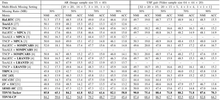
CLUSTERING RESULTS(AVERAGENORMALIZEDMUTUALINFORMATION(NMI)ANDCLUSTERINGACCURACY(ACC)%)ON THEARFACIAL IMAGES ANDUSFGAIT VIDEOS WITH{30%,50%,70%,90%}MISSING ENTRIES UNDER MULTI-BLOCK MISSING SETTINGS.
Data AR (Image sample size55×40) USF gait (Video sample size64×44×20) Multi-Block Missing Setting {20×20, 16×7, 3×10,1×1} {32×20×10,20×15×5, 4×3×4,1×1×1}
Missing Ratio (MR) 30% 50% 70% 90% 30% 50% 70% 90%
Metric NMI ACC NMI ACC NMI ACC NMI ACC NMI ACC NMI ACC NMI ACC NMI ACC
HaLRTC[25] 51.5 17.5 48.5 15.8 49.0 15.4 46.6 15.0 49.7 19.0 48.7 17.5 48.9 16.1 48.5 15.5 TenALS[27] 50.1 15.9 48.2 15.3 45.2 13.3 42.5 12.6 – – – – – – – – TNCP[26] 51.1 17.8 48.9 15.8 46.3 14.8 45.6 14.3 49.2 18.2 48.2 16.6 48.5 16.3 48.1 15.2 HaLRTC +MPCA[3] 49.6 17.6 48.6 15.8 46.6 15.4 44.8 15.0 49.7 19.8 48.8 16.3 48.2 14.9 48.1 14.9 TenALS +MPCA[3] 50.2 16.3 47.4 15.1 44.4 13.7 41.8 12.7 – – – – – – – – TNCP +MPCA[3] 50.0 16.0 49.0 15.1 47.2 14.8 46.1 13.8 50.3 19.0 48.9 16.8 48.4 15.5 48.0 14.9 HaLRTC +SOMPCARS[6] 52.0 18.1 50.6 17.4 47.7 15.6 45.6 14.8 49.6 20.0 47.8 18.1 45.7 17.2 45.4 16.7 TenALS +SOMPCARS[6] – – – – – – – – – – – – – – – – TNCP +SOMPCARS[6] 50.8 16.7 48.5 15.2 47.3 15.0 46.0 14.1 50.3 20.0 48.5 17.4 48.2 17.2 47.6 15.9 HaLRTC +LRANTD[4] 50.8 16.5 49.2 15.8 47.9 15.7 46.3 15.6 49.7 18.7 48.3 15.9 48.5 15.3 48.3 15.3 TenALS +LRANTD[4] 50.6 16.7 47.9 15.5 45.2 13.9 43.3 13.7 – – – – – – – – TNCP +LRANTD[4] 51.2 17.3 49.8 16.4 48.3 15.1 45.9 14.8 49.7 18.7 49.2 16.6 49.2 16.1 48.1 15.2 TRPCA[11] 45.8 12.9 42.7 12.4 39.1 11.7 36.1 10.8 48.2 18.2 47.0 15.2 46.0 15.2 45.8 13.8 SSC[43] 46.3 13.9 46.3 13.3 45.8 13.1 45.5 13.0 49.4 19.4 47.0 16.3 45.9 15.2 45.2 14.3 SSC-CEC[21] 48.1 14.3 47.6 13.4 47.5 13.0 46.5 12.1 44.4 14.6 44.4 13.5 – – – – ZF + SSC[21] 48.8 15.0 48.5 14.2 47.7 13.5 47.6 13.2 50.0 19.4 48.6 16.8 47.9 15.7 46.7 13.8 SRME-MC[22] 49.1 15.6 47.3 12.3 47.3 12.1 47.1 11.8 50.0 19.3 47.4 15.6 47.1 14.8 47.0 14.6 TDVM-Tucker 85.8 65.1 84.2 61.8 83.2 61.6 82.1 58.8 90.0 75.4 88.4 71.8 88.2 71.8 87.6 70.3 TDVM-CP 84.2 59.6 82.3 54.8 79.2 48.7 77.0 45.4 87.4 68.4 86.5 67.7 85.5 65.8 82.8 64.3
compared methods such as HaLRTC + LRANTD, TNCP and TNCP + LRANTD also achieve good results especially in the cases of MR≤ 70%, these state-of-the-art methods cannot maintain good performance with increasing missing data (MR > 70%). In this scenario, TDVM-CP achieves the best performance although it extracts only 10 features from each video sample. Moreover, TenALS and its combined “two-step” strategies fail to work on the higher-order dataset (Weizmann).
3) Face/Gait Clustering: For clustering tasks, we test on AR facial images (55 ×40×1200) and USF gait videos (64×44×20×731). To measure the clustering performance, we adopt two metrics: Normalized Mutual Information (NMI) and Clustering Accuracy (ACC). Table III shows that TDVM-Tucker and TDVM-CP still outperform all other methods, including the four state-of-the-art clustering methods. Al-though these subspace clustering methods have shown good performance in the original papers, they do not achieve good results (and even fail to work on a few cases in which MR ≥ 70%) on these incomplete tensors probably because they are not applicable in this scenario (i.e., tensors with multi-block missing). Here, TDVM-Tucker achieves the best clustering results in all cases followed closely by TDVM-CP. In terms of NMI, TDVM-Tucker and TDVM-CP outperform the other methods by at least 36.7% and33.5% on average on the AR dataset, and this improvement increases to over
40.5% and 37.5% on average on the USF gait database, respectively. In terms of ACC, the results of the 17 compared methods are worse than those of measuring in NMI, while TDVM-Tucker and TDVM-CP achieve much better clustering accuracy, particularly on the gait videos with55.8%and50.1%
improvements on average, respectively.
4) Time Cost: We report the average time cost of feature extraction in Appendix B of the Supplementary Material. TDVM-Tucker is faster than the compared methods in most
cases although our implementations are not optimized for efficiency as our focus here is accuracy. TDVM-CP is slightly slower than TDVM-Tucker because it requires more iterations to achieve convergence. Besides, HaLRTC, TNCP and TRPCA are more efficient than other existing methods, while certain two-step strategies such as TenALS + MPCA/LRANTD are very time consuming (more than 50 times slower than TDVM). Nevertheless, the efficiency can be improved, for example, by using sparse implementations in future work.
D. Summary of Experimental Results
– The proposed methods, TDVM-Tucker and TDVM-CP, outperform the 17 competing methods with 15.3% to
75.5% improvements in all cases of face recognition, object/action classification and face/gait clustering on six real-world image and video datasets. With more missing entries, our methods show more advantages with much better results than other methods. These results verify the effectiveness and superiority of incorporating low-rank tensor decomposition with feature variance maximization.
– TDVM-Tucker and TDVM-CP consistently achieve good results regardless of various multi-block missing set-tings and parameters. Besides, our methods also demon-strate its stability and superiority with respect to feature dimension reduction, benefitting from low-rank (low-dimensional) tensor decomposition. Although TDVM-CP yields the best results in fewer cases than TDVM-Tucker, it extracts low-dimensional vector features resulting in more dimensionality reduction. TDVM-CP, therefore, not only provides informative features but also reduces more time cost and memory space for further application (e.g., classification).
– HaLRTC, HaLRTC + LRANTD and HaLRTC + SOM-PCARS are the best performing existing algorithms on the whole in Tables I, II and III respectively. TNCP