Dynamic Contrast-Enhanced MRI of the
Patellar Bone: How to Quantify Perfusion
Dirk H.J. Poot, PhD,
1,2* Rianne A. van der Heijden, MD, PhD,
3,4Marienke van Middelkoop, PhD,
4Edwin H.G. Oei, MD, PhD,
3and
Stefan Klein, PhD
1Purpose:To identify the optimal combination of pharmacokinetic model and arterial input function (AIF) for quantitative analysis of blood perfusion in the patellar bone using dynamic contrast-enhanced magnetic resonance imaging (DCE-MRI).
Materials and Methods:This method design study used a random subset of five control subjects from an Institutional Review Board (IRB)-approved case–control study into patellofemoral pain, scanned on a 3T MR system with a contrast-enhanced time-resolved imaging of contrast kinetics (TRICKS) sequence. We systematically investigated the reproduc-ibility of pharmacokinetic parameters for all combinations of Orton and Parker AIF models with Tofts, Extended Tofts (ETofts), and Brix pharmacokinetic models. Furthermore, we evaluated if the AIF should use literature parameters, be subject-specific, or group-specific. Model selection was based on the goodness-of-fit and the coefficient of variation of the pharmacokinetic parameters inside the patella. This extends previous studies that were not focused on the patella and did not evaluate as many combinations of arterial and pharmacokinetic models.
Results:The vascular component in the ETofts model could not reliably be recovered (coefficient of variation [CV] ofvp >50%) and the Brix model parameters showed high variability of up to 20% forkelacross good AIF models. Compared to group-specific AIF, the subject-specific AIF’s mostly had higher residual. The best reproducibility and goodness-of-fit were obtained by combining Tofts’ pharmacokinetic model with the group-specific Parker AIF.
Conclusion: We identified several good combinations of pharmacokinetic models and AIF for quantitative analysis of perfusion in the patellar bone. The recommended combination is Tofts pharmacokinetic model combined with a group-specific Parker AIF model.
Level of Evidence:2
Technical Efficacy:Stage 1
J. MAGN. RESON. IMAGING 2018;47:848–858.
R
esearch suggests that altered blood perfusion of the patellar bone may play a role in the pathogenesis of patellofemoral pain (PFP), a common knee complaint.1–8 Blood perfusion can be visualized and analyzed quantita-tively using dynamic contrast-enhanced magnetic resonance imaging (DCE-MRI).9Despite the well-described use of DCE-MRI for a variety of indications such as tumors and cerebral strokes,10,11 only a limited number of publications address DCE-MRI in bone,12–16 and none specifically in the patella. DCE-MRI in bone has been limited due to the sparse vascular-ization of bone and the typical low contrast enhancementcompared to surrounding tissues.12,16 The mobility of the patella poses an additional specific challenge.
Signal intensity changes in the DCE-MRI time series are due to the contrast medium entering the tissue through feeding arteries, residing in the extravascular space, and sub-sequent draining. This process can be studied semiquantita-tively using measures like time-to-peak, or quantitasemiquantita-tively by fitting a pharmacokinetic model to the DCE-MRI data to extract truly quantitative measures of perfusion.9Quantitative DCE-MRI requires choosing one of multiple proposed arte-rial input functions (AIFs) and one of the pharmacokinetic
View this article online at wileyonlinelibrary.com. DOI: 10.1002/jmri.25817 Received Mar 17, 2017, Accepted for publication Jun 29, 2017.
*Address reprint requests to: D.H.J.P., Erasmus MC, Na2516, Depts. of Medical Informatics & Radiology, Biomedical Imaging Group Rotterdam, P.O. Box 2040, 3000 CA Rotterdam, The Netherlands. E-mail: d.poot@erasmusmc.nl
From the1Biomedical Imaging Group Rotterdam, Departments of Medical Informatics & Radiology, Erasmus MC, Rotterdam, The Netherlands; 2Quantitative Imaging, Department of Imaging Physics, Delft University of Technology, Delft, The Netherlands;3Department of Radiology & Nuclear
Medicine, Erasmus MC, Rotterdam, The Netherlands; and4Department of General Practice, Erasmus MC, Rotterdam, The Netherlands
Additional supporting information may be found in the online version of this article.
This is an open access article under the terms of the Creative Commons Attribution-NonCommercial License, which permits use, distribution and reproduction in any medium, provided the original work is properly cited and is not used for commercial purposes.
models that together are able to describe the dynamic contrast concentration. Selection of appropriate models is especially rel-evant for low signal intensity regions since a too complex model (too many degrees of freedom) will be influenced stronger by acquisition noise and, hence, is less sensitive to between-group or between-subject differences in perfusion. Moreover, a model that cannot describe the DCE-MRI signal with sufficient accuracy may fail to detect relevant changes in perfusion. Although quantitative DCE-MRI has been per-formed in several bones,9no thorough evaluation of the opti-mal combination of AIF and a pharmacokinetic model has been presented. Due to the differences in perfusion, the model evaluation results obtained on tumor tissue are not directly applicable to the analysis of patellar perfusion.17
The aim of this study was to identify the optimal combination of pharmacokinetic model and AIF for quanti-tative analysis of perfusion in the patellar bone using DCE-MRI. As potentially appropriate AIF models we selected three models by Orton et al18 and several parametrizations of Parker et al’s model.19 As pharmacokinetic models we selected the models of Brix, Tofts, and the extended model of Tofts.20
Materials and Methods
DCE-MRI Acquisition
This method design study used a random subset of five control subjects and five patients from an Institutional Review Board
(IRB)-approved case–control study into patellofemoral pain con-taining 134 subjects.21All subjects provided written informed
con-sent. A 3T MRI scanner (Discovery MR750, GE Healthcare, Milwaukee, WI) with a dedicated 8-channel knee coil (Invivo, Gainesville, FL) was used.
DCE-MRI was acquired by a time-resolved imaging of con-trast kinetics (TRICKS) sequence with anterior–posterior (AP) fre-quency encoding direction to avoid pulsation artifacts of the popliteal artery into the region of interest. MRI parameters were: in-plane pixel resolution 1.5 mm, slice thickness 5 mm, field of view 380 3 380 3 70 mm, acquisition matrix 256 3 128, 14 sagittal slices, 70% sampling in the phase direction, echo time (TE) 5 1.7 msec, repetition time (TR) 5 9.3 msec, flip angle (FA) 5 308. The DCE-MRI protocol consisted of 35 phases of 10.30 6 0.07 sec (constant within subject). Intravenous contrast administration of 0.2 mmol/kg gadopentetate dimeglumine (Mag-nevist, Bayer, Berlin, Germany), at a rate of 2 ml/s, was started after the first phase. Additionally, a nonfat-suppressed 3D SPGR sequence with in-plane resolution of 0.33 0.3 mm and 0.5 mm slices was acquired before contrast administration for delineation of the patellar bone marrow. See Figs. 1 and 2 for an example image of a control subject and a patient, respectively.
Motion Compensation
Image-driven motion compensation was applied, based on a tech-nique developed for T1mapping in femoral and tibial articular
car-tilage.22 A registration mask was drawn around the patella in the 3D SPGR image. Within this mask the DCE-MRI time series were automatically registered to the first DCE-MRI timepoint FIGURE 1: Example DCE image at maximum arterial enhancement in one of the control subjects, time intensity curve, and fit with Tofts’ model, including the overlays showing the apparent heterogeneity inside the patella.
using a rigid transformation model. Subsequently, the first phase was registered to the 3D SPGR image and all DCE-MRI scans were transformed to the grid of the high-resolution 3D SPGR. Visual inspection indicated successful alignment of the time series. Quantitative DCE-MRI Modeling
The dynamic DCE-MRI signal in each voxelA(t)is described by a combination of three models: The AIF, the pharmacokinetic response function (P), and the function that relates contrast con-centration to signal intensity (S), combined as:
AðtÞ5SnðAIFvP/ÞðtÞ (1) wheredenotes convolution andn,v,uare model parameters.
For the AIF model we evaluated three computationally efficient models of Orton et al18 (Orton1, Orton2, Orton3), five variations on Parker et al’s model19with increasing degrees of free-dom (Parker-L, Parker-A, Parker-S, Parker-E, Parker-T), as well as a “dummy” triangle-shaped AIF function. The AIF parameters v
were estimated from a manually outlined arterial region, either from a single subject (subject-specific) or from the entire group of subjects (group-specific), or obtained from the literature ( literature-based).
For the pharmacokinetic model P we evaluate Brix, Tofts, and Extended Tofts (ETofts) models.20,23The Brix model hasAH, kep, andkelas parametersu, while Tofts model hasKtransandkepas
u, and ETofts adds vp to it; each model additionally includes a
delay parameter.
ForSwe used a standard model suitable for the SPGR based sequence with one free parametern5S0.
The Supplementary Material sections S.1–S.3 provide more details on the models and section S.4 provides details on the maxi-mum likelihood estimation method used to recover n, v, and u
with constraints provided in Table 1.
Technical Validation on Phantom Data
To validate the model fitting method, a simulated dataset from a DCE-MRI anthropomorphic digital reference phantom was used.24 This phantom, designed to validate fitting methods, contains a simulation of perfusion inside a brain tumor, which was selected as the volume-of-interest (VOI). All AIF models were fitted on selected arterial voxels and evaluated with the R-square value. Sub-sequently, these AIFs were used to analyze the provided VOI with ETofts. Accuracy of the pharmacokinetic parameters was measured by the median absolute difference (MAD) between the estimated and ground truth parameters of the ETofts model in the VOI and compared to the median ground truth value.
Comparative Evaluation of AIF Models
The AIF models were fitted to the voxels in a region of interest (ROI) drawn in the center of the popliteal artery, approximately at the level of the center of the patella. This artery was the largest artery in the field of view and could easily be identified in all sub-jects. Fit quality was evaluated by Akaike’s information criterion (AIC)25,26:
FIGURE 2: Example DCE image at maximum arterial enhancement in one of the patients, time intensity curve, and fit with Tofts’ model, including the overlays showing the apparent heterogeneity inside the patella.
AIC52k1nlnðSSRÞ (2) where k is the number of parameters in the model (for all sub-jects), n is the number of samples to which the model is fitted, andSSR is the sum of squared residuals (measurements minus val-ues predicted by the fitted model). AIC provides an objective way to compare models with different complexities. Since the voxels from which the AIF is estimated are selected from a small region, they have substantial spatial correlation, which reduces the effective number of degrees of freedom. To avoid a biased model selection due to these correlations, we evaluated the AIC on one randomly selected voxel within the arterial ROI of each subject, and we report the mean and standard deviation of the AIC over 1000 ran-dom selections.
Comparative Evaluation of Pharmacokinetic Models
Each combination of AIF and pharmacokinetic model was fitted to the DCE-MRI data. For each pharmacokinetic parameter we com-puted its weighted mean over a VOI consisting of the patellar bone marrow, drawn by an experienced observer (R.H.). As weights we used 1/CRLB where CRLB is the Cramer-Rao lower bound at each voxel, which is a measure of fit uncertainty (see Supporting Information S.4). In this way, we suppress the influ-ence of voxels with an unreliable fit. The mean and coefficient of variation (CV5 standard deviation /jmeanj) across subjects were computed to investigate reproducibility. The residual (5pffiffiffiffiffiffiffiffiSSR) was computed to evaluate goodness-of-fit.
TABLE 1. Parameters, Units, and Constraints Applied During Estimation
Model All Tofts and ETofts ETofts Brix
parameter delay Ktrans kep vp AH kep kel
unit min (min)-1 (min)-1 (fraction) min-2 (min)-1 (min)-1
Lower bound optimization 0 -0.1 -1 -0.1 -0.2 -1 0
Lower bound initialization 0.17 -0.01 -0.2 -0.001 -0.05 -0.2 0.2
Upper bound initialization 2.50 0.5 0.5 0.001 0.25 0.8 4
Upper bound optimization 5 1 3 0.2 1 3 10
TABLE 2. Median Absolute Difference (MAD) of ETofts Parameters in the VOI of the Phantom Experiment for the Different AIF Models
Ktrans(1/min) kep(1/min) vp(fraction)
Literature-based Triangle 0.1986 0.345 0.0155 Orton1 0.0696 0.459 0.0111 Orton2 0.0672 0.466 0.0059 Orton3 0.0081 0.446 0.0074 Parker 0.0133 0.468 0.0079 Subject-specific Triangle 0.5461 0.387 0.0379 Orton1 0.0696 0.459 0.0111 Orton2 0.0695 0.032 0.0126 Orton3 0.0293 0.043 0.0107 Parker-A 0.0118 0.082 0.0092 Parker-S 0.0059 0.070 0.0047 Parker-E 0.0096 0.085 0.0058 Parker-T 0.0079 0.086 0.0011
Median ground truth 0.0701 0.418 0.0138
FIGURE 3: Literature-based, subject-specific, and group-specific arterial contrast concentration, from left to right, top to bottom: Literature, Orton1, Orton2, Orton3, Parker-A, Parker-S, Parker-E, Parker-T. In each figure, the group-specific estimate is shown by the black bold line.
TABLE 3. Mean (SD) of the AIC of AIF Fits
Literature-based Subject-specific Group-specific
Triangle 2636.0 (14.6) 1999.8 (14.2) 1987.9 (13.3) Orton1 1906.7 (21.6) 1365.6 (12.3) 1346.9 (15.1) Orton2 1963.2 (10.9) 560.8 (21.5) 751.8 (38.0) Orton3 1308.5 (17.3) 605.9 (19.6) 793.5 (33.8) Parker-L 1348.8 (16.1) Parker-A 576.6 (24.4) 756.1 (35.8) Parker-S 454.4 (36.5) 725.4 (42.2) Parker-E 244.7 (52.6) 662.0 (47.9) Parker-T 297.3 (54.6) 640.2 (53.8)
RESULTS
Technical Validation on Phantom Data
On the phantom data, the Parker-T model fitted best to the arterial signal with an R-square value of 0.9994, whereas Parker-E and Orton3 had R-square of 0.9983 and 0.9876, respectively. Orton3 fitted best among the Orton models. See Table 2 for the MAD of Ktrans, kep, and vp inside the
VOI. Parker-T had the lowest MAD forKtrans andvp.
Comparative Evaluation of AIF Models
Figure 3 shows the AIFs that were estimated by the different models. There were substantial differences between AIFs when estimated for each subject individually, especially for the models Orton2, Orton3, and Parker-A. The substantial
differences in contrast concentration in the tail of the curve were observed to be correlated to under/overestimation of the baseline signal intensity n. For subject-specific Parker-E and Parker-T, the first-pass contrast concentration differed substantially from the group-specific pass and the first-pass as provided by the literature-based AIFs. The group-specific Parker-T was also substantially different from the literature-based Parker model.
Table 3 shows the mean and standard deviation of the AIC value of the AIF fits over the 1000 random selections of one voxel per subject. Note that in Eq. (2),n5175 (35 timepoints 3 1 randomly selected voxel 3 5 subjects) and k varies between 20 (literature-based AIF; only estimating delay andnper subject) and 123 (subject-specific Parker-T). TABLE 4. For Each AIF and Pharmacokinetic Model, the Mean Over the Five Control Subjects of Each Parameter and the Residual
Tofts Extended Tofts Brix Residual
Ktrans kep Ktrans kep vp AH kep kel Tofts ETofts Brix
Literature-based Triangle 0.057 20.133 0.050 20.139 0.000 0.127 0.023 0.464 0.119 0.119 0.070 Orton1 0.023 0.112 0.021 0.116 0.000 0.059 0.255 1.415 0.083 0.081 0.069 Orton2 0.025 0.123 0.021 0.125 0.000 0.062 0.284 1.407 0.081 0.081 0.069 Orton3 0.016 0.148 0.014 0.151 0.000 0.035 0.215 1.430 0.079 0.079 0.069 Parker 0.015 0.131 0.014 0.134 0.000 0.037 0.313 0.954 0.081 0.081 0.069 Subject-specific Triangle 0.770 20.157 0.756 20.163 0.050 0.924 0.009 0.249 0.146 0.147 0.114 Orton1 0.035 0.211 0.029 0.203 0.004 0.057 0.234 2.148 0.074 0.073 0.073 Orton2 0.014 0.106 0.013 0.041 0.000 0.029 0.246 1.594 0.084 0.074 0.070 Orton3 0.005 0.095 0.005 0.097 0.000 0.011 0.229 1.306 0.085 0.086 0.068 Parker-A 0.008 0.127 0.007 0.131 0.000 0.017 0.254 1.195 0.084 0.084 0.069 Parker-S 0.015 0.160 0.013 0.161 0.000 0.032 0.210 1.259 0.080 0.079 0.069 Parker-E 0.015 0.191 0.013 0.193 0.000 0.030 0.233 1.856 0.076 0.076 0.069 Parker-T 0.014 0.177 0.012 0.180 0.000 0.030 0.250 1.664 0.077 0.077 0.068 Group-specific Triangle 0.752 20.139 0.734 20.145 0.053 0.883 20.056 0.488 0.132 0.132 0.105 Orton1 0.031 0.219 0.025 0.207 0.004 0.050 0.296 1.724 0.074 0.072 0.073 Orton2 0.020 0.212 0.017 0.213 0.000 0.041 0.302 1.589 0.075 0.075 0.069 Orton3 0.004 0.071 0.004 0.075 0.000 0.008 0.155 1.198 0.088 0.089 0.068 Parker-A 0.007 0.136 0.007 0.139 0.000 0.015 0.199 1.212 0.080 0.079 0.069 Parker-S 0.015 0.197 0.014 0.198 0.000 0.032 0.262 1.367 0.076 0.076 0.069 Parker-E 0.014 0.187 0.012 0.189 0.000 0.028 0.236 1.490 0.075 0.075 0.069 Parker-T 0.014 0.181 0.011 0.184 0.000 0.027 0.230 1.799 0.076 0.076 0.069
Ktrans,kep,kelin 1/min;vpis a fraction;AHis in 1/min2; residual norm is in arbitrary units but it can be compared across all model
The AIC of Parker-E and Parker-T were much lower than the AIC of the Orton models. All models substantially improved over the triangle AIF.
Comparative Evaluation of Pharmacokinetic Models
Tables (4–7) show the mean and CV across control subjects and across patients of the pharmacokinetic parameters, as well as of the residual norm, for all combinations of AIF and pharmacokinetic models.
Variations in parameter values for different AIF mod-els were observed, both for controls (Table 4) and patients (Table 6); eg, 20% difference in Brix kel between
group-specific Parker E&T. The residual of ETofts was not sub-stantially lower than the residual of Tofts, which indicates
that, in our patellar VOI, inclusion of the vascular compo-nent did not lead to a better fit. This is additionally reflected in that the vascular fractionvpis close to zero. For
most AIF models, the residual of the Brix model was10% lower than the residual of Tofts and ETofts. The residual norm did not vary substantially across AIF models, except for the “dummy” Triangle AIF and the literature-based AIFs combined with the ETofts model, which resulted in a higher residual norm.
Table 5 shows that for the control subjects the pharma-cokinetic parameters estimated with subject-specific AIF mod-els had an increased CV compared to pharmacokinetic parameters estimated with literature-based and group-specific AIF models. For most combinations there were only small differences in CV of the parameters between literature-based TABLE 5. For Each AIF and Each Parameter of the Pharmacokinetic Models, the CV (%) Over the Five Control Subjects
Tofts Extended Tofts Brix Residual
Ktrans kep Ktrans kep vp AH kep kel Tofts ETofts Brix
Literature-based Triangle 62.9 231.4 70.0 220.1 82.2 23.9 492.7 79.1 20.5 20.7 14.9 Orton1 35.5 27.3 52.4 26.5 2165.5 30.7 43.5 61.9 16.5 16.4 15.9 Orton2 35.6 24.5 48.7 23.2 436.8 35.7 61.0 60.8 15.9 16.5 15.8 Orton3 32.4 23.9 40.0 22.8 2249.6 32.8 28.4 50.0 15.9 16.2 16.2 Parker 36.8 24.0 45.4 23.9 188.0 31.5 41.7 73.9 16.2 16.4 16.1 Subject-specific Triangle 32.9 216.4 34.5 214.3 77.3 6.8 1120.1 127.8 25.4 25.2 23.4 Orton1 23.7 27.3 36.8 28.9 61.4 28.4 26.0 31.6 15.3 15.3 16.1 Orton2 57.1 223.2 53.3 950.9 636.6 60.5 32.4 47.7 35.7 15.9 16.1 Orton3 52.5 40.9 53.9 39.8 2514.8 45.6 76.9 44.3 16.6 17.0 16.7 Parker-A 53.2 53.1 46.1 50.1 249.9 58.8 51.5 51.8 18.6 19.7 16.2 Parker-S 53.8 79.3 52.9 79.3 3897.8 49.5 69.4 60.1 17.2 17.4 15.9 Parker-E 19.7 25.5 27.6 25.3 199.9 24.1 32.0 20.0 17.5 18.2 15.2 Parker-T 27.3 22.5 31.1 21.7 583.9 28.1 28.8 31.9 16.6 17.1 15.9 Group-specific Triangle 23.2 218.8 25.5 216.9 78.8 8.8 2108.3 43.3 24.7 24.4 22.6 Orton1 26.2 16.8 38.4 17.9 56.8 29.6 43.8 62.3 15.3 15.2 15.9 Orton2 27.6 20.2 43.3 19.3 2420.5 32.2 28.0 44.8 15.7 16.0 15.7 Orton3 33.8 56.3 40.4 53.0 335.0 29.3 43.1 46.7 18.4 18.8 16.5 Parker-A 34.3 28.7 40.4 28.2 497.9 31.7 34.2 48.5 16.6 17.0 16.5 Parker-S 28.8 21.1 38.8 20.1 2713.5 32.4 32.9 54.6 15.9 16.2 16.2 Parker-E 29.3 22.8 42.0 22.1 8001.0 32.4 25.6 45.3 15.3 15.7 15.4 Parker-T 29.3 23.3 44.2 22.7 21748.7 32.1 27.8 19.8 15.4 15.9 15.5 The three right-most columns show the CV of the residual.
and group-specific AIF models. The exceptions were kep of
Tofts and ETofts with Orton3,vp of ETofts, andkep and kel
of Brix with Orton2, Orton3, and Parker, which were mostly found to have a higher CV for the group-specific AIF. When comparing the CV of the different models we noted that over-all the CV for the Tofts’ model was lower than the CV for the other models. Especially, the CV ofKtranswas substantially
larger in ETofts than Tofts. For ETofts, the CV ofvpwas very
high, demonstrating that the vascular component could not be precisely recovered, caused by the close to zero vp (Table
4). The CV of the Brix model parameters was, overall, higher than the CV of the Tofts model parameters. The CV in patients (Table 7) was higher than in control subjects.
Discussion
This article presents a systematic comparative evaluation of AIF and pharmacokinetic models for quantitatively analyz-ing patellar perfusion with DCE-MRI.19 Below, we derive several recommendations based on our results, and discuss the strengths, limitations, and impact.
The evaluation of digital phantom data shows that the proposed fitting method can accurately recover pharmacoki-netic parameters when a correct AIF model is used. Although this phantom dataset simulates tumor perfusion,24 which dif-fers from patellar perfusion, the comparison with the ground truth confirms the technical validity of the proposed fitting methods.
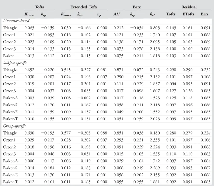
TABLE 6. For Each AIF and Pharmacokinetic Model, the Mean Over the Five Patients of Each Parameter and the Residual
Tofts Extended Tofts Brix Residual
Ktrans kep Ktrans kep vp AH kep kel Tofts ETofts Brix
Literature-based Triangle 0.063 20.159 0.050 20.166 0.000 0.212 20.034 0.803 0.163 0.161 0.091 Orton1 0.021 0.093 0.018 0.102 0.000 0.121 0.233 1.740 0.107 0.104 0.088 Orton2 0.023 0.109 0.020 0.114 0.000 0.138 0.171 2.095 0.105 0.103 0.089 Orton3 0.014 0.133 0.013 0.135 0.000 0.073 0.276 2.138 0.100 0.100 0.086 Parker 0.013 0.112 0.012 0.115 0.000 0.075 0.214 1.818 0.103 0.104 0.086 Subject-specific Triangle 0.652 20.220 0.545 20.227 0.081 0.874 20.072 0.243 0.290 0.290 0.232 Orton1 0.030 0.207 0.024 0.193 0.007 0.290 0.215 2.132 0.101 0.097 0.106 Orton2 0.019 0.201 0.017 0.201 0.001 0.111 0.229 1.837 0.094 0.093 0.091 Orton3 0.004 0.037 0.003 0.035 0.000 0.017 0.098 1.607 0.127 0.126 0.085 Parker-A 0.003 0.039 0.003 20.002 0.000 0.017 0.118 1.523 0.125 0.118 0.085 Parker-S 0.012 0.170 0.011 0.167 0.000 0.058 0.211 2.118 0.097 0.096 0.086 Parker-E 0.011 0.159 0.009 0.157 0.000 0.049 0.200 1.552 0.097 0.095 0.085 Parker-T 0.010 0.155 0.009 0.151 0.001 0.051 0.259 2.023 0.099 0.097 0.085 Group-specific Triangle 0.630 20.193 0.577 20.203 0.088 0.851 0.038 0.180 0.280 0.279 0.224 Orton1 0.029 0.217 0.023 0.202 0.007 0.293 0.221 2.335 0.101 0.097 0.106 Orton2 0.018 0.198 0.016 0.198 0.001 0.091 0.229 2.224 0.093 0.091 0.088 Orton3 0.004 0.048 0.003 0.051 0.000 0.015 0.105 1.535 0.110 0.110 0.083 Parker-A 0.006 0.117 0.006 0.119 0.000 0.029 0.164 1.742 0.097 0.097 0.084 Parker-S 0.014 0.184 0.012 0.183 0.001 0.068 0.219 2.269 0.093 0.093 0.087 Parker-E 0.013 0.170 0.011 0.171 0.001 0.058 0.202 2.155 0.092 0.091 0.086 Parker-T 0.012 0.164 0.011 0.165 0.000 0.055 0.255 1.881 0.092 0.091 0.085
Ktrans,kep,kelin 1/min;vpis a fraction;AHis in 1/min2; residual norm is in arbitrary units but it can be compared across all model
As indicated by the AIC scores, Triangle and Orton1 do not model the arterial signal well. For the Parker model, the increase in complexity from Parker-A to Parker-E is sup-ported by the measured imaging data, since Parker-E leads to substantially improved arterial fits, reflected by lower AIC. This indicates that our addition of a persisting contrast concentration to the Parker-E model was justified. Overall, in terms of AIC, the most competitive models are Orton2, Parker-E, and Parker-T.
The AIC score shows substantially improved arterial fits of the subject and group-specific AIFs compared to the literature-based AIF. Moreover, except for Orton3, the literature-based AIFs lead to higher residuals when used in combination with the (E)Tofts pharmacokinetic model. Based on these results, we recommend against using a literature-based AIF.27
Since the large intersubject variability in the shape of the first-pass contrast concentration for subject-specific AIF modeling with Parker-E and Parker-T, and to a lesser extent with Orton2 and Orton3, cannot be explained biologically, similar to Ref. 28, the group-specific AIF is preferred for these models, despite the higher AIC value. Note that for Parker-E&T the CV of Ktrans and AH is higher for the
group-specific AIF than for the subject-specific AIF, while it is lower for kep. This suggests that components of the AIF
relevant for determining Ktrans can be recovered from an
individual subject with a higher precision than the intersub-ject variation, whereas those components more relevant to determinekepcannot.
Comparing pharmacokinetic models, the CV typically is lowest for Tofts. This is probably due to the larger num-ber of parameters in ETofts and Brix. The larger numnum-ber of TABLE 7. For Each AIF and Each Parameter of the Pharmacokinetic Models, the CV (%) Over the Five Patients
Tofts Extended Tofts Brix Residual
Ktrans kep Ktrans kep vp AH kep kel Tofts ETofts Brix
Literature-based Triangle 107.8 240.6 108.9 233.1 93.2 70.0 2409.6 50.2 46.4 46.2 25.4 Orton1 84.3 99.6 94.6 88.7 2120.9 85.1 18.0 58.8 25.6 24.8 23.2 Orton2 83.9 89.1 92.8 84.1 2175.4 89.3 76.4 31.4 24.5 24.2 23.2 Orton3 87.1 76.6 92.7 75.6 2356.5 87.1 29.9 49.4 22.7 23.0 22.3 Parker 91.2 86.5 94.1 83.3 359.9 85.4 24.5 68.0 24.0 24.1 22.6 Subject-specific Triangle 52.9 240.5 71.2 236.9 88.7 16.1 2199.9 67.1 83.7 83.5 80.8 Orton1 69.1 65.5 94.4 64.1 96.2 116.3 67.6 38.5 24.2 23.0 32.6 Orton2 100.9 71.9 119.3 70.9 140.8 128.4 75.7 72.4 20.7 20.4 25.4 Orton3 153.4 456.9 154.0 474.1 123.3 141.7 178.2 67.5 41.1 42.4 23.5 Parker-A 110.5 384.5 118.6 29638.5 150.9 88.3 140.4 51.7 26.1 30.4 23.0 Parker-S 79.4 86.1 93.9 90.4 159.2 78.8 85.6 38.1 20.5 20.4 23.0 Parker-E 83.8 89.7 101.8 94.0 151.7 79.3 84.4 67.9 20.4 20.1 22.7 Parker-T 83.9 87.6 102.2 93.0 108.5 77.0 20.9 54.4 17.0 16.9 23.0 Group-specific Triangle 51.0 239.5 64.0 236.3 76.4 17.0 328.8 84.6 90.1 89.7 84.3 Orton1 74.0 54.1 94.5 53.5 80.5 119.4 54.0 28.5 24.2 23.2 31.7 Orton2 81.2 59.2 94.4 58.8 91.5 94.8 62.0 32.3 21.8 21.6 22.6 Orton3 91.2 175.7 96.0 165.3 22921.1 78.2 114.0 41.3 26.4 26.8 22.5 Parker-A 87.4 83.2 94.9 81.8 107.7 82.9 77.2 57.1 21.8 22.0 22.6 Parker-S 82.7 61.9 94.6 61.9 72.8 90.8 63.6 35.6 21.5 21.6 22.4 Parker-E 83.8 64.0 95.1 64.0 81.9 88.8 66.1 39.6 21.3 21.4 21.8 Parker-T 84.4 65.5 94.1 65.5 70.9 88.1 82.3 57.9 21.2 21.4 21.9 The three right-most columns show the CV of the residual.
parameters in Brix may also explain the 10% lower residual compared to Tofts. As all three pharmacokinetic models explain a similar fraction of the DCE-MRI signal, we expect that group differences, eg, between cases and controls, in perfusion cause similar relative changes in parameter values. This implies that the model with the smallest CV (Tofts) will likely be more sensitive to detect group differences than the other models (ETofts, Brix).
We chose to aggregate the voxel-wise pharmacokinetic measures by computing a weighted mean over the patella VOI. Any spatial heterogeneity within the patella is thus averaged out. Hence, it should be noted that using these measures to study group differences implicitly assumes non-localized physiological changes in the patella.
As no in vivo ground truth values for pharmacokinetic parameters are available, we could not base model selection on closeness to ground truth, and this implies that reliable absolute quantification of perfusion values currently cannot be claimed. As in Schmid et al,17 we used a statistical analy-sis method to trade off model complexity against goodness-of-fit, in order to guide model selection. Note that, com-pared to Schmid et al, we evaluated a wider range of mod-els, both for AIF and for pharmacokinetic model, and applied it to patellar DCE-MRI data.
The substantial differences in pharmacokinetic param-eters obtained with different AIFs emphasize the relevance of choosing a good AIF model. Severe bias in parameters could occur with a suboptimal AIF. The small differences observed among the best candidates indicate that potentially other combinations can be best for acquisitions with differ-ent settings and/or in differdiffer-ent body parts; even for other bones. Hence, our proposed framework for evaluating perfu-sion is an important contribution in itself. It allowed identi-fication of a few combinations of AIF models and pharmacokinetic models that performed well in all aspects: AIC score and biological credibility of the AIF, CV of phar-macokinetic parameters, and goodness-of-fit in the patella VOI. Given the similarity in perfusion mechanisms and MR characteristics, we would expect these combinations to also perform well when studying perfusion in other bones such as tibia,12femur,16hip,14or bony pelvis.15
Although Orton2 combined with the Tofts’ model seems to slightly improve reproducibility and goodness-of-fit in this dataset, we consider the lower AIC score of Parker-T as well as the improved biological credibility of that AIF to be more important. Together with the accuracy of this com-bination on phantom data, this gives good confidence that group-specific Parker-T combined with the Tofts’ model is suitable to identify patellar perfusion abnormalities.
The observed values of the CV indicate that with a consistently used combination of models, reproducibility is sufficient to allow identification of group differences in perfu-sion with reasonably sized groups; eg,40 subjects per group
allow identification of group differences of 10% in Ktrans or kepat a significance level ofP<0.05 with 75% power.
In conclusion, the most suitable choice of models for the analyzed patellar DCE-MRI data is Parker’s arterial input model, where all parameters of Parker’s model are esti-mated from arterial voxels of the full group of subjects, combined with Tofts’ pharmacokinetic model.
Acknowledgment
Contract grant sponsor: Hitachi Medical Systems/RSNA Research Seed Grant 2014; contract grant number: RSD1440 EUR fellowships: “Robust Quantitative MRI With Precision Estimates” and “Penetrating Patellofemoral Pain: A Cross-Sectional Case-Control Study.”
References
1. Arnoldi CC, Lemperg RK, Linderholm H. Intraosseous hypertension and pain in the knee. J Bone Joint Surg Br 1975;57b:360–363. 2. Hejgaard N, Diemer H. Bone scan in the patellofemoral pain
syn-drome. Int Orthop 1987;11:29–33.
3. LaBrier K, O’Neill DB. Patellofemoral stress syndrome. Sport Med 1993;16:449–459.
4. N€aslund JE, Odenbring S, N€aslund U-B, Lundeberg T. Diffusely increased bone scintigraphic uptake in patellofemoral pain syndrome. Br J Sports Med 2005;39:162–165.
5. N€aslund J, Walden M, Lindberg L-G. Decreased pulsatile blood flow in the patella in patellofemoral pain syndrome. Am J Sports Med 2007;35:1668–1673.
6. Ho KY, Hu HH, Colletti PM, Powers CM. Recreational runners with patellofemoral pain exhibit elevated patella water content. Magn Reson Imaging 2014;32:965–968.
7. Lemperg RK, Arnoldi CC. The significance of intraosseous pressure in normal and diseased states with special reference to the intraosseous engorgement-pain syndrome. Clin Orthop Relat Res 1978;143–156. 8. Selfe J, Harper L, Pedersen I, Breen-Turner J, Waring J, Stevens D. Cold
legs: A potential indicator of negative outcome in the rehabilitation of patients with patellofemoral pain syndrome. Knee 2003;10:139–143. 9. Dyke JP, Aaron RK. Noninvasive methods of measuring bone blood
perfusion. Ann N Y Acad Sci 2010;1192:95–102.
10. Li SP, Padhani AR. Tumor response assessments with diffusion and perfusion MRI. J Magn Reson Imaging 2012;35:745–763.
11. Copen WA, Schaefer PW, Wu O. MR perfusion imaging in acute ischemic stroke. Neuroimaging Clin N Am 2011;21:259–283. 12. Seah S, Wheaton D, Li L, et al. The relationship of tibial bone perfusion
to pain in knee osteoarthritis. Osteoarthr Cartil 2012;20:1527–1533. 13. Lee JH, Dyke JP, Ballon D, Ciombor DM, Rosenwasser MP, Aaron RK.
Subchondral fluid dynamics in a model of osteoarthritis: use of dynamic contrast-enhanced magnetic resonance imaging. Osteoarthr Cartil 2009;17:1350–1355.
14. Lee JH, Dyke JP, Ballon D, Ciombor DM, Tung G, Aaron RK. Assess-ment of bone perfusion with contrast-enhanced magnetic resonance imaging. Orthop Clin North Am 2009;40:249–257.
15. Breault SR, Heye T, Bashir MR, et al. Quantitative dynamic contrast-enhanced MRI of pelvic and lumbar bone marrow: Effect of age and marrow fat content on pharmacokinetic parameter values. Am J Roentgenol 2013;200:297–303.
16. Budzik JF, Lefebvre G, Forzy G, El Rafei M, Chechin D, Cotten A. Study of proximal femoral bone perfusion with 3D T1 dynamic contrast-enhanced MRI: a feasibility study. Eur Radiol 2014;24:3217–3223.
17. Schmid VJ, Whitcher B, Yang G-Z, Taylor NJ, Padhani AR. Statistical analysis of pharmacokinetic models in dynamic contrast-enhanced magnetic resonance imaging. Med Image Comput Comput Assist Interv 2005;8(Pt 2):886–893.
18. Orton MR, d’Arcy JA, Walker-Samuel S, et al. Computationally effi-cient vascular input function models for quantitative kinetic modelling using DCE-MRI. Phys Med Biol 2008;53:1225–1239.
19. Parker GJM, Roberts C, Macdonald A, et al. Experimentally-derived functional form for a population-averaged high-temporal-resolution arterial input function for dynamic contrast-enhanced MRI. Magn Reson Med 2006;56:993–1000.
20. Tofts PS. Modeling tracer kinetics in dynamic. J Magn Reson Imaging 1997;7:91–101.
21. Van Der Heijden RA, Oei EHG, Bron EE, et al. No difference on quan-titative magnetic resonance imaging in patellofemoral cartilage com-position between patients with patellofemoral pain and healthy controls. Am J Sports Med 2016;44:1172–1178.
22. Bron EE, Van Tiel J, Smit H, et al. Image registration improves human knee cartilage T1 mapping with delayed gadolinium-enhanced MRI of cartilage (dGEMRIC). Eur Radiol 2013;23:246–252.
23. Brix G, Semmler W, Port RE, Schad L, Gunter L, Lorenz WJ. Pharma-cokinetic parameters in CNS Gd-DTPA enhanced MR imaging. J Comput Assist Tomogr 1991;15:621–628.
24. Bosca RJ, Jackson EF. Creating an anthropomorphic digital MR phan-tom—an extensible tool for comparing and evaluating quantitative imaging algorithms. Phys Med Biol 2016;61:974.
25. Akaike H. A new look at the statistical model identification. IEEE Trans Autom Control 1974;19:716–723.
26. Ardekani BA, Kershaw J, Kashikura K, Kanno I. Activation detec-tion in funcdetec-tional MRI using subspace modeling and maximum likelihood estimation. IEEE Trans Med Imaging 1999;18:101– 114.
27. Fedorov A, Fluckiger J, Ayers GD, et al. A comparison of two meth-ods for estimating DCE-MRI parameters via individual and cohort based AIFs in prostate cancer?: A step towards practical implementa-tion. Magn Reson Imaging 2014;32:321–329.
28. Hormuth DA, Skinner JT, Does MD, Yankeelov TE. A comparison of individual and population-derived vascular input functions for quantitative DCE-MRI in rats. Magn Reson Imaging 2014;32:397– 401.