SLA Definition for Multi-tenant DBMS and its Impact on Query Optimization

HAL Id: hal-02319756

https://hal.archives-ouvertes.fr/hal-02319756

Submitted on 18 Oct 2019

HAL

is a multi-disciplinary open access

archive for the deposit and dissemination of

sci-entific research documents, whether they are

pub-lished or not. The documents may come from

teaching and research institutions in France or

abroad, or from public or private research centers.

L’archive ouverte pluridisciplinaire

HAL, est

destinée au dépôt et à la diffusion de documents

scientifiques de niveau recherche, publiés ou non,

émanant des établissements d’enseignement et de

recherche français ou étrangers, des laboratoires

publics ou privés.

SLA Definition for Multi-tenant DBMS and its Impact

on Query Optimization

Shaoyi Yin, Abdelkader Hameurlain, Franck Morvan

To cite this version:

Shaoyi Yin, Abdelkader Hameurlain, Franck Morvan. SLA Definition for Multi-tenant DBMS and its

Impact on Query Optimization. IEEE Transactions on Knowledge and Data Engineering, Institute

of Electrical and Electronics Engineers, 2018, 30 (11), pp.2213-2226. �10.1109/TKDE.2018.2817235�.

�hal-02319756�

Any correspondence concerning this service should be sent

to the repository administrator:

[email protected]

This is an author’s version published in:

http://oatao.univ-toulouse.fr/22381

To cite this version: Yin, Shaoyi and Hameurlain,

Abdelkader and Morvan, Franck SLA Definition for

Multi-tenant DBMS and its Impact on Query Optimization. (2018)

IEEE Transactions on Knowledge and Data Engineering, 30

(11). 2213-2226. ISSN 1041-4347

Official URL

DOI :

https://doi.org/10.1109/TKDE.2018.2817235

Open Archive Toulouse Archive Ouverte

OATAO is an open access repository that collects the work of Toulouse

researchers and makes it freely available over the web where possible

SLA

Definition

for

Multi-Tenant

DBMS

and

its

Impact

on

Query

Optimization

Shaoyi

Yin

,

Abdelkader

Hameurlain

,

and

Franck

Morvan

Abstract—Inthecloudcontext,usersareoftencalledtenants.AcloudDBMSsharedbymanytenantsiscalledamulti-tenantDBMS. TheresourceconsolidationinsuchaDBMSallowsthetenantstoonlypayfortheresourcesthattheyconsume,whileprovidingthe opportunityfortheprovidertoincreaseitseconomicgain.Forthis,aServiceLevelAgreement(SLA)isusuallyestablishedbetween theproviderandatenant.However,inthecurrentsystems,theSLAisoftendefinedbytheprovider,whilethetenantshouldagreewith itbeforeusingtheservice.Inaddition,onlytheavailabilityobjectiveisdescribedintheSLA,butnottheperformanceobjective.Inthis paper,anSLAnegotiationframeworkisproposed,inwhichtheproviderandthetenantdefinetheperformanceobjectivetogetherin afairway.Todemonstratethefeasibilityandtheadvantageofthisframework,weevaluateitsimpactonqueryoptimization.Weformally definetheproblembyincludingthecost-efficiencyaspect,wedesignacostmodelandstudytheplansearchspaceforthisproblem, werevisetwosearchmethodstoadapttothenewcontext,andweproposeaheuristictosolvetheresourcecontentionproblemcaused byconcurrentqueriesofmultipletenants.Wealsoconductaperformanceevaluationtoshowthat,ouroptimizationapproach(i.e.,driven bytheSLA)canbemuchmorecost-effectivethanthetraditionalapproachwhichalwaysminimizesthequerycompletiontime.

IndexTerms—Cloudcomputing,cost-efficiency,multi-tenancy,queryoptimization,servicelevelagreement

1

I

NTRODUCTION

A

multi-tenant DBMS can be used by a PaaS (Platform as a Service) provider to manage the data of all its custom-ers (which become tenants in the cloud context). This kind of service is often called DBaaS (Database as a Service). As in any other cloud-based service, the resource consolidation allows the tenants to only pay for the resources that they consume (pay-as-you-go), while providing the opportunity for the provider to increase its economic gain. Examples of such systems include MS SQL Azure [23], Amazon RDS [2] and Oracle Data Cloud [17]. With these systems, a Service Level Agreement (SLA) is established between the provider and a tenant. However, they are often defined by the pro-vider, while the tenant should agree with it before using the service. In addition, only the availability objective is described in the SLA of these services, but not the perfor-mance objective. Indeed, defining perforperfor-mance objectives and above all, guaranteeing them is very challenging. Data-base queries have different levels of complexity, so defining a unique performance objective for all queries is not realistic.

In the research community, some work [13], [19] has intro-duced the performance SLO (Service Level Objective) to the DBaaS systems, for OLTP applications [13] and for OLAP applications [19] respectively. In this paper, we are interested in OLAP applications. Similar to but slightly different from

[19], we will include the performance objective in the SLA by fixing a threshold for each query template1and associate a price to it. In order to do so, we will define a negotiation framework such that the tenant and the provider could define this threshold together in a rather fair way. The aim is to find a performance objective that is satisfactory or at least acceptable by the tenant and reachable (i.e., technically achievable and financially profitable) for the provider. In the SLA, we also fix the pricing policy, which is used to adjust the price according to the real performance and the parame-ter values. If the query answer is delayed or the query is rejected, a penalty should be paid by the provider.

In a multi-tenancy environment, the performance for an individual tenant can be degraded because of the interfer-ence of other tenants. Guaranteeing the satisfaction of a ten-ant in terms of performance is a critical problem. A possible solution is to enforce performance isolation [16], [6], i.e., to specify the performance objective in the SLA by fixing the absolute amount of required resources (e.g., CPU, I/O, memory, and network) and the penalty in case of violation. This solution requires a lot of responsibility from the tenant: the tenant has to know in advance how many resources will be needed for its query, which is a very difficult task with OLAP applications. Thus, in our work, we will define the SLA in a different way such that the tenant does not need to know the resource consumption in advance. During the SLA negotiation, the tenant only provides the query templates with some basic statistics, and it is the provider who is responsible for estimating the resource requirements of a query in order to propose a reasonable price. Then, ! The authors are with the IRIT Laboratory, Paul Sabatier University,

118RoutedeNarbonne,ToulouseCedex931062,France. E-mail:{yin,hameurlain,morvan}@irit.fr.

DigitalObjectIdentifierno.10.1109/TKDE.2018.2817235

1.A query template is a parameterized SQL query, i.e., to use varia-bles instead of constant values in the selection predicates, as can be seen in the TPC-H benchmark.

controlling the real resource consumption for a specific query becomes an important task of the query optimizer.

Once the SLA is defined, the objective of the query opti-mizer is to find an execution plan for a given query such that the performance expectation of the tenant is satisfied and the economic benefit of the provider is maximized. Sometimes, the optimizer detects that there are not enough resources to reach the performance objective, or that the eco-nomic benefit could be negative. In these cases, the opti-mizer should decide whether to wait for resources to be released, or to reject the query, or to start the current query but suspend other running queries which are relatively less beneficial. In other words, the query optimizer should be revisited to solve these problems.

The contributions of this paper are: (1) we define a frame-work which allows a fair negotiation between both the provider and the tenant. The tenant prepares a test case containing a small set of query templates, specifying a per-formance expectation for each template, and the provider proposes a pricing function with regard to the real perfor-mance and the parameter values. The tenant could compare offers from different providers and choose the most appro-priate one; (2) we study the impact of the SLA on query optimization to demonstrate the feasibility and the advan-tage of our framework. We formally define the problem by taking into account the economic aspects. We revise the cost model, the search space and some search methods to adapt to the new context. We also propose a heuristic to solve the resource contention problem caused by concurrent queries of multiple tenants.

The rest of the paper is organized as follows. Section 2 analyzes the related work. Section 3 defines the SLA negoti-ation framework. Section 4 studies the impact on query optimization, including the problem formulation, a cost model, the search space and two search methods. Section 5 shows the experimental results. Finally, Section 6 concludes the paper and points out future work.

2

R

ELATED

W

ORK

As said above, in this paper, we deal with two main chal-lenges: (1) the SLA definition for multi-tenant DBMS, which takes into account the performance objectives, and (2) cost-effective query optimization. Below, we study the related work corresponding to these two directions.

2.1 Performance Concerned SLA Definition

In the DBaaS context, [13] is one of the first research work which takes the performance SLO into consideration for query processing. This work has been done for OLTP applications and the performance metric is transactions per second (tps). Two types of SLO are distinguished: (1) H, associated with a high performance of 100 tps and (2) L, associated with a lower performance of 10 tps. The authors present a frame-work that takes as input the tenant frame-workloads, their perfor-mance SLOs, and the available hardware resources, and outputs a cost-effective recipe that specifies how much hard-ware to provision and how to schedule the tenants on each hardware resource.

A recent work [19] which focuses on OLAP applications introduces the notion of Personalized Service Level

Agreement (PSLA). The main idea is that a tenant should specify the database schema with basic statistics (e.g., base table cardinalities), and then the cloud provider shows dif-ferent levels (tiers) of services that can be provided. Each service tier contains a set of query templates, the estimated performance for each template and the price (dollars/hour) corresponding to this level of service. The advantage is that the tenant does not need to specify its query templates in advance, but only needs to choose a service level. However, PSLA has some constraints. In fact, each defined service tier is generated based on a specific hardware configuration, for example, a shared-nothing architecture with 4 nodes, 6 nodes or 8 nodes. Thus, inside a tier, the performance degrades with the complexity of the query. Once the tier is chosen, a tenant cannot expect a good scalability (i.e., hav-ing more or less the same performance for simple and com-plex queries by allocating different amounts of resources).

In our paper the target workload is OLAP applications, and the performance metric is the Query Completion Time (QCT)2. Unlike in [19], we allow a tenant to specify an expected performance threshold for each query template independently, and each query will be invoiced separately. It is the query optimizer of the provider which decides how many resources should be dedicated to a given query and issues performance isolation if necessary. Indeed, the tenant has to provide in advance a small set of query templates that he will make. However, in the context of OLAP applica-tions, this is not a hard problem.

2.2 Monetary-Cost-Aware Query Optimization Some research work treats monetary-cost-aware query opti-mization as a multi-objective optiopti-mization problem [27]. QCT and Monetary Cost (MC) are defined as independent cost metrics. The query optimizer tries to find the best trade-off.

Algorithms like Dynamic Programming (DP) [21] that prune plans based on a single cost metric rely on the follow-ing principle of optimality: replacfollow-ing subplans within a query plan by better subplans with regard to that cost metric cannot worsen the entire query plan. This principle breaks when there are multiple cost metrics [7]. Based on that insight, Ganguly et al. [7] proposed an extended DP algorithm that uses a multi-objective version of the principle of optimality. This algorithm guarantees to generate optimal query plans. However, it is too computationally expensive for practical use, as shown in [27]. Thus, Trummer et al. [27] proposed two approximation schemes for multi-objective query opti-mization problem which formally guarantee to return near-optimal query plans while speeding up optimization by several orders of magnitude in comparison with exact algo-rithms. However, as we will demonstrate in Section 4.4.1, when the parallelism of query execution is considered, the pruning strategy used in [7] and [27] becomes invalid.

Kllapi et al. [12] also tackled the problem of multi-objective optimization, but it focuses on the resource allocation phase of data processing flows in the cloud. The authors propo-sed some heuristics bapropo-sed on greedy algorithms and simu-lated annealing [8] to find the optimal schedule for three types of problems: (1) minimize QCT given a fixed budget,

2.QCT is defined to be the elapsed time between the query submis-sion and the return of the complete result (Section 4.1).

(2) minimize MC given a deadline, and (3) find trade-offs between QCT and MC without any a-priori constraints. Indeed, resource allocation is also an important step in query optimization. However, it is not the focus of our paper. We deal mainly with the join order determination problem, as in [27].

Although multi-objective optimization is relevant to our work, it is a general approach, and for our specific problem described in Section 1, we think that it is more appropriate to define it as a single objective optimization problem. We try to maximize the provider’s benefit, while treating the query completion time threshold and the maximum resource consumption as constraints to meet. The reason of doing this is twofold: first, the tenant does not need to choose a plan from a set of proposed plans for each query. Thus, the query processing is transparent; second, the constraints can be used by the optimizer to prune some intermediate results, so that the search method is more efficient, as will be shown in Section 5.5.

3

S

LA

N

EGOTIATION

F

RAMEWORK

In the existing SLAs for DBaaS systems, the performance objective (i.e., the QCT) is not explicitly described [3], [18], [22]. The main reasons are as follows. First, even if the ten-ant may have a rough expectation for theQCT, it is not sure that this expectation could be met by the provider. Second, if we let the provider define the QCT threshold and the price, it may trick the tenant. In fact, the commonly used pricing policy is that the price is a function of the consumed resources. However, for a database query, the resource con-sumption depends on the execution plan chosen by the opti-mizer. If the optimizer chooses a bad plan, not only will the

QCTbe larger, but also the bill will be higher, which is not fair for the tenant. Therefore, neither the tenant nor the pro-vider should decide alone the performance objective and the corresponding price for a query. In this section, we will define a framework which allows a fair negotiation between both sides. The negotiation is aided by an automated Offer Generation Tool (OGT) at the provider’s side. The design of a good OGT is not trivial. It should follow some guidelines: (1) the generated offer should be simple enough so that the tenant can easily understand it, (2) the defined performance objective should be reachable by the provider for any instantiated query, (3) the defined objectives should be auditable by the tenant, and (4) the communication during the negotiation between the provider and the tenant should be minimized.

The main idea of our negotiation framework is as fol-lows. For each template, the tenant specifies an expected

QCTðQCTEXPÞ and a tolerance threshold '. The OGT estimates the shortest QCTðQCTSÞ with the correspond-ing price, and the lowest price with the correspondcorrespond-ing

QCT. IfQCTEXP is smaller thanQCTS, the expectedQCT will be automatically adjusted to QCTS. Then, the OGT defines a price function with regard to the actual QCT. The tenant could compare this offer with the offers from other providers. Once the provider is chosen, the tenant can add new query templates whenever he wants, and the OGT can automatically extend the SLA. Note that the statistics the tenant provides may be inaccurate so the

estimation may be irrelevant. In this case, a renegotiation may be triggered. These steps will be discussed in detail in Section 3.1. An example will be given in Section 3.2. 3.1 Steps for Generating the SLA Offer

The main steps are explained in detail below.

Step 1: Fixing the QCT threshold for each query tem-plate.The input to the OGT includes: (a) the schema of the database (i.e., relations, attributes, data types, and con-straints, etc.), (b) the estimated number of tuples in each base relation, (c) a set of query templates with parameter-ized predicates (as in the benchmark TPC-H), (d) aQCTEXP and a tolerance threshold'for each template, and (e) some other statistics that are needed to estimate cadinalities of intermediate results (e.g., numbers of distinct values of the attributes), if available. If (e) is not provided by the tenant, the OGT will use some default values. The inaccuracy prob-lem is addressed inStep 4.

For each query template, the OGT first supposes the highest selectivity for each parameter and calculates the fol-lowing information, by running its query optimizer: (1) the shortest query completion timeQCTS and the correspond-ing pricePRS, and (2) the lowest pricePRLand the

corre-sponding query completion timeQCTL.

IfQCTEXPis smaller thanQCTS, the expectedQCTwill be automatically adjusted to QCTS. For example, for a given query template, the tenant has an initial expected query completion time, which is 15s. If the optimizer returns the following result: QCTS ¼5s, PRS ¼50cents; QCTL¼10s,

PRL¼5cents, then the threshold 15s will be maintained, and the price will be 5 cents. However, if the optimizer returns:

QCTS¼20s, PRS ¼30cents; QCTL¼50s, PRL¼5cents, then the tenant‘s expectation will be adjusted automatically by the OGT to 20s.

If QCTS %QCTEXP %QCTL, the corresponding price

PREXPis fixed by using the following function:

PREXP ¼PRLþ

PRs'PRL

QCTL'QCTS

(ðQCTL'QCTEXPÞ: (1)

For the last example, if the threshold was 30s, then according to this function, the expected price is 22 cents.

Step 2: Defining the price function with regard to the real QCT. A na€ıve pricing policy could be that: if the real

QCT is not larger thanQCTEXP, the provider returns back the query result and the tenant will be billed with the expected price; otherwise, the provider does not give back the result and pays a penalty instead. However, we find it too strict. In fact, very often, the tenant could tolerate a small delay if the price is reduced correspondingly. Thus, in our framework, we allow the tenant to define a factor ' such that a penalty is only paid ifQCT > ')_QCT

EXP. More pre-cisely, the following function is applied to compute the price to be invoiced (denoted byPRSLA):

PRSLA¼

PREXP; if QCT% QCTEXP

!QCT_EXP QCT

"

(PREXP; if QCTEXP < QCT%'(QCTEXP

'PREXP; if QCT > '(QCTEXP 8 > < > : : (2)

This is illustrated by Fig. 1. Once the price functions are defined, the tenant compares them with the offers from other providers and chooses the best one for him.

We define the price as a piecewise function with respected to theQCT value, but it does not mean that each point is achievable, since the solutions for a query are dis-crete points. However, we think that it is not a problem, and the most important thing is that the way that we fix the

QCTthreshold and define the price function is fair for both sides. On the one hand, the tenant cannot trick the provider to acquire a penalty by defining a lower QCTEXP. First, as said above,QCTEXP cannot be smaller thanQCTS, so there is always a chance that the provider meets the threshold. Second, if the tenant picks a lowQCTEXP and the provider meets it, the tenant has to pay a high price. Thus, the best strategy for the tenant is to show his expectation honestly. On the other hand, the provider cannot trick the tenant by offering higher PRS and PRL either, due to the pressure that the tenant may choose another provider.

Step 3: Varying the price according to the selectivity.

Since the price PREXP in Step 1 is computed by supposing the highest selectivity for each parameter, there might be an overpricing problem. To avoid this, it is better to define a finer pricing function with respect to the selectivity for each parameter. However, unfortunately, such a function can be extremely complex, especially when there are multiple parameters in a query template. In order to make a tradeoff between the fairness and the ease of comprehension, we propose to compute three expected prices (PREXP LOW,

PREXP MEDIUM and PREXP HIGH) corresponding to three levels of selectivity: low, medium and high. For example, if a query template contains two parameters X and Y, the selectivity interval of X is [0.1, 0.5] and the selectivity inter-val of Y is [0.3, 0.9], then the OGT will estimate three prices: for example, 10 cents for (0.1, 0.3), 30 cents for (0.3, 0.6), and 100 cents for (0.5, 0.9).

For a specific query, when we generate the invoice, we will compute the Euclidean distances between its selectivity vector and the three pre-defined vectors respectively. The one with the shortest distance decides the price.

Step 4: Renegotiating and extending the SLA. The reli-ability of the OGT relies on the cost model of the query opti-mizer, especially the cardinality estimation module. In fact, cardinality estimation is itself a complicated subject which has been well-studied in the literature [14], [1]. With the pro-posed techniques, estimation errors can be reduced but are still inevitable. Therefore, we accept that the first estimation of the OGT can be inaccurate. This is not a problem for the tenant, because the main objective of the initial negotiation is

to compare offers from different providers. Since all pro-viders receive the same statistics, the comparison remains valuable. However, for the provider, it may cause some financial loss. Our solution is to periodically detect the esti-mation inaccuracy by using execution traces and propose a renegotiation if it is significant enough (e.g., the overall eco-nomic loss during the last month reaches 5 percent due to this inaccuracy). During the renegotiation, since the OGT can extract exact cardinalities from the execution traces, the new cost estimations become much more accurate. The pro-vider can even get refunded for the past queries. Of course, the refunding policy should be written clearly in the SLA to avoid that malicious tenants refuse to be responsible. The execution traces can be used by the tenant to prepare a new test case to see if other providers could propose cheaper offers. Evidently, the provider should minimize the renegoti-ation risk. A possible track is to adapt robust query optimiza-tion methods [28] to the cloud context.

Another case is that the database grows with time, so the statistics become obsolete. In this case, the provider can update the SLA periodically without renegotiations. The tenant is not obliged to check each updated version of the SLA, but he can make a control whenever he wants.

As said before, once the initial SLA is established, it can be dynamically extended. That is to say, new templates can be added at any moment and the corresponding price func-tions will be generated immediately. Thus, ad-hoc queries can be handled easily. To insure that the provider treats new query templates equally with those defined in the ini-tial SLA, he is obliged to provide a detailed invoice and nec-essary execution traces for each query, so the tenant can carry out an audit process if in doubt. To insure the credibil-ity of the traces, fraud detection techniques should be designed. However, in our paper, we do not address this issue.

3.2 An Example

Let us consider the query template given in Step 3. The OGT uses the query optimizer to make estimates and gets the following information: for the highest selectivity, the short-est time QCTS¼52sand PRS¼150 cents; the lowest price

PRL¼50 centsandQCTL¼60s.

We assume that the expected QCTof the tenant is 56s and the tolerance factor is 2. Then, QCTEXP is accepted as 56s and the expected price for the high selectivity is 100 cents. After that, the optimizer estimates the lowest prices for medium and low selectivities, under the con-straint of QCT <¼56s. Suppose that they are 30 cents and 10 cents.

Now, let us consider a query with selectivity vector (0.3, 0.7). Normally, the provider could answer it in at most 56s and the price should be 30 cents. However, if the provider is overloaded and answers the query in 80s, the tenant will accept it, even though he is less satisfied. The good news is that he only needs to pay a bill of 21 cents.

4

I

MPACT ON

Q

UERY

O

PTIMIZATION

In order to meet the defined SLA while maximizing the provider’s benefit, in this section, we reformulate the query

optimization problem and revisit the principle components of the query optimizer.

4.1 Problem Formulation

In this study, we assume that the database server is a paral-lel DBMS running on top of a shared-nothing architecture. We deal with SPJ (Select-Project-Join) queries, which are the most frequent queries in OLAP applications. Thus, a query

Qcan be represented as a connected graph, where each ver-tex is a relation, and each edge is a join predicate.

Before defining the optimization problem, we first intro-duce some important cost metrics for a query execution plan.

Query Completion Time (QCT): the elapsed time between the query submission and the return of the complete result.

Maximum Parallelism Degree (MPD):the maximum num-ber of nodes occupied at the same time during the query execution.

Monetary Cost (MC): the economic cost with regard to resource consumption.

MC¼X

N

i¼1

DRi (PRNodeþVtr(PRnet; (3)

where N is the number of nodes used for the query execu-tion,DRi is the duration thatNode i is occupied,PRNodeis the monetary cost of a node during a time unit (e.g., cents/s),PRnetis the monetary cost of the network to trans-fer a bit, andVtris the total volume of data (number of bits) transferred during query execution.

Note that theMC is the monetary cost for the provider, but not the price provided to the tenant. In order to have some benefit, the provider defines a gain factor aða > 0Þ, and the proposed price is:

PR¼ ð1þaÞ )MC: (4)

When the query is submitted, the optimizer needs to esti-mate the economic benefit of each plan with regard to the defined SLA. Thus, we add the following metric:

Unit Benefit Factor (UBF):the average benefit in a time unit.

UBF ¼ðPRSLA'MCÞ=QCT: (5)

Using the above cost metrics, we define our problem as follows:

SLA-driven Cost-effective Query Optimization is a process which finds, for a query Q, the execution plan P that maximizes the UBF, while satisfying the conditionsQCTðPÞ <¼QCT th

andMPDðPÞ <¼MPD th, where:

QCT(P) and MPD(P) are the QCT and MPD of the plan P, respectively;

QCT_th is the threshold of the query completion time

ðQCT th¼')_QCT EXPÞ;

and MPD_th is the maximum number of nodes that can be used to execute the query, which is decided by the system’s resource manager according to the current load.

Note that the query optimization cost is not negligible. It has an impact on theQCT, theMCand thus theUBF. How-ever, this cost cannot be considered directly by the optimiza-tion process. Therefore, we divide the problem into two steps: the first step is to choose an appropriate search method

which minimizes the optimization cost; and the second step is to find the optimal plan by using the chosen method.

Compared to a traditional query optimization problem which simply minimizes the QCT, our problem is more complex. First, the objective function is specific, so the cost model needs to be redesigned (see Section 4.2), the existing search space restriction rules need to be rechecked (see Sec-tion 4.3). Then, due to the constraint checks, pruning strate-gies like Dynamic Programming (DP) often used by classical enumerative search methods cannot work effi-ciently. This will be seen in Section 4.4.1. In order to make the optimization process more efficient, we will also revise a randomized search method in Section 4.4.2. Finally, it is possible that no solution can be found for our optimization problem when there is a resource contention caused by con-current queries of other tenants. We will propose a heuristic to solve the resource contention problem in Section 4.4.3.

We point out that maximizing the UBF for each query does not mean the maximization of provider’s overall profit in a long term. However, it can be seen as a greedy strategy. In Section 5, we will experimentally show that, with our proposal, the overall profit can truely be increased, com-pared to the traditional approach which does not consider the economic aspects.

4.2 Cost Model

To illustrate our proposal, we use a classical execution model: a query execution plan is represented as a binary operator tree, and the join algorithm is parallel hash join [11], [20]. Details are given in Section 4.2.1. The reason to choose this model is that, our target applications are OLAP queries, which deal with huge volumes of data, and execut-ing a sexecut-ingle query usually requires multiple nodes runnexecut-ing in parallel. For simplicity, we assume that the nodes are homogeneous. We also assume that queries from the same tenant are launched sequentially. Actually, concurrent queries from a tenant are much more difficult to take care of, because they share the same data. Either they should be serialized to avoid data migration, or some data should be (statically or dynamically) replicated to increase the par-allelism. We will study this problem deeply in future work.

Obviously, new cost models should be designed when other execution models are used. For example, new multi-way join operators and data shuffling algorithms have been proposed recently in [4] which aim to reduce the communi-cation cost for complex multi-join queries. This section can be served as an example for designing other cost models. 4.2.1 Query Execution Paradigm

A query execution plan is represented as an operator tree. The relationship between two operators could be: (i) sequential, meaning that one operator cannot start until the other one finishes, (ii) independent, so both operators can be executed in parallel, or (iii) pipelinable, meaning that one operator consumes the output of the other operator and they are executed in parallel. Thus, the plan tree can be seen as a set of pipeline chains (PC). At a given time, if all the inputs of a PC are available (i.e., the preceding operators are all executed), this PC is called an executable pipeline chain (EPC).

The relationships between operators can be represented through an operator dependency graph [20]. Fig. 2 shows an operator tree (left side) and the corresponding depen-dency graph (right side). A PC is enclosed by a dashed line. A dependency between PCs is represented by a bold directed arc. [20] proposed the following scheduling strat-egy for this example operator tree:

Seq Par

Pipescan R2 – build R2End_Pipe Pipescan R1 – build R1End_Pipe End_Par

Pipescan R3 – probe R2 – probe R1End_Pipe End_Seq

This operator scheduling model can be generalized using the notion of pipeline chains defined above, as shown in Fig. 3. Thereafter, an iteration will be called an execution phase (EP).

To summarize, a query plan is executed in a sequence of phases. An execution phase contains one or more pipeline chains, which are executed in parallel. A pipeline chain has one or more physical operators, which are executed in pipeline. In addition, a physical operator is executed by multiple nodes in parallel (i.e., intra-operation parallelism). Note that, at any given moment, a resource is used by only one query, and there is no interference of other queries. We argue that the resource isolation [16] is very important to make the estimation more accurate, and above all, to avoid unexpected SLA violations.

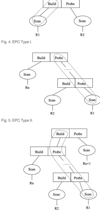
In order to estimate the cost of a query plan, we distin-guish the following three types of executable pipeline chains (see Figs. 4, 5, and 6). Type I: Scan-Build (a scan oper-ator followed by a build operoper-ator), Type II:

Scan-Probe-. Scan-Probe-. Scan-Probe-.-Probe (a scan operator followed by one or more probe operators), and Type III: Scan-Probe-. . .Probe-Build (a scan operator followed by one or more probe operators and then by a build operator).

To make the analysis more concise, we can further general-ize these three types of EPCs into the following form:Scan' (Probe))'(Build), where () means the operation is optional, and)means the operation can be repeated. Consequently, in section 4.2.3, we will give only the cost formulas for Type III. Those for Type I and Type II can easily be extracted.

4.2.2 Parameters

The parameters of the cost model and some values that we will use are listed in Table 1. The relation Rx is ini-tially distributed on dd_x nodes. The data placement problem is outside of our scope. An algorithm can be found in [5]. For simplicity, we choose the values of the parametersdd xandpdxin such a way that all data par-titions could fit into the main memory during the query execution.

Note that the price of the data storage is not included in our cost model, because the data storage cost is independent of the query optimization problem.

Fig. 2. An operator tree and its dependency graph.

Fig. 3. Generalized operator scheduling model.

Fig. 4. EPC Type I.

Fig. 5. EPC Type II.

4.2.3 Cost Estimation

We first give the cost model for a PC of Type III, then for an execution phase, and finally for the complete query.

For a PC of Type III.The scan operator and the build oper-ator are executed in pipeline by different nodes. The elapsed time of a scan operator is the sum of the time to load the data into memory, the time to execute the select operator and the time to prepare the tuple partitioning. The time of transferringbbytes of data fromNnodes toMnodes is esti-mated using the following formula:

Ttr¼ðb= Mð )NÞ=nbþndÞ)MAX N; Mð Þ: (6)

For example, in Fig. 7, there is 60 MB data stored on 3 nodes. Suppose that the network bandwidthnb¼10 GB=s

and the network delay is 1 ms. Thus, the time for transfer-ring the data to 2 nodes is 6 ms. In fact, each destination node has to receive sequentially 3 packages of 10 MB, which constitutes a bottleneck.

Based on this formula, we estimate the elapsed time for a PC of type III as follows:

Elapsed

Elapsed timetime ETET ¼

MAXðET Scan Rð 1Þ;ET Transfer Rð 1Þ;ET Probe Rð 1Þ; . . . ;ET Transfer Rð 12 . . .ðn'1ÞÞ;ET ProbeðR12 . . .ðn'1ÞÞ;

ET Transfer Rð 12 . . .nÞ;ET Build Rð 12 . . .nÞÞ; where ET ScanðR1Þ ¼

ET ScanðR1Þ ¼

SUMðjR1j)jS1j=dd1=dbþdl;==read the pages from disk R1

j j)jS1j)ipc=dd1=cpu;==executethe select operator

sðR1Þ

j j)jS1j)iph=dd 1=cpu

==prepare the tuple partitioningÞ;

ET Transfer ET Transfer RðR11Þ¼¼ sðR1Þ j j)jS1j= dd_ð 1)_{pd 2Þ=nbþnd} ð Þ)max ddð 1;pd2Þ; ET ProbeðR1Þ ¼ ET ProbeðR1Þ ¼

SUMðjsðR1Þj)jS1j)iph=pd2=cpu;==execute the probe R12

j j)jS12j)iph=pd12=cpu

==prepare the repartitioningÞ;

ET TransferðR12 . . .ðn'1ÞÞ ¼ ET TransferðR12 . . .ðn'1ÞÞ ¼ jR12 . . .ðn'1Þj)jS12 . . .ðn'1Þj=ðpd ðn'1Þ)pd nÞ=nbþndÞ )_{maxðpdðn'1Þ;pd nÞ;} ET Probe ET Probe RðR12 . . .12 . . .ðnn''11ÞÞ¼¼

SUMðjR12 . . .ðn'1Þj)jS12 . . .ðn'1Þ)iphj=pd n=cpu;

==to execute the probe operator R12 . . .n

j j)jS12 . . .nj)iph=pd n=cpu

==to prepare the tuple repartitioningÞ;

ET Transfer ET Transfer RðR12 . . .12 . . .nnÞ¼¼ ðjR12 . . .nj)jS12 . . .nj= pd n_ð )_{pd 12 . . .nÞ=nbþndÞ} )_{max pd nð ;pd12 . . .nÞ;} ET BuildðR12 . . .nÞ ¼ ET BuildðR12 . . .nÞ ¼ R12 . . .n j j)jS12 . . .nj)iph=pd12 . . .n=cpu: (7)

The transferred data volume is:

TDVTDV ¼jsðR1Þj)jS1j þjR12j)jS12j þ + + + þjR12 . . .ðn'1Þj)

S12 . . .ðn'1Þ

j j þjR12 . . .nj)jS12 . . .nj:

(8) The maximum number of occupied nodes is:

MNNMNN ¼dd 1þXn_i¼2pd iþpd12 . . .n: (9)

For an execution phaseEPi composed of k pipeline chains:

EPi¼ fPC1; PC2;. . .; PCkg.

These pipeline chains are executed in parallel, so the elapsed time of an execution phase is computed like:

ET

ET EðEPPiiÞ ¼MAX ET PCð ð 1Þ;ET PCð 2Þ; . . . ;ET PCð kÞÞ: (10)

The transferred data volume is the sum of theTDVof all pipeline chains: TDVTDV EðEPPiiÞ ¼ Xk j¼1TDV PCj ! " : (11)

The maximum number of occupied nodes is:

MNNMNN EPiðEPiÞ ¼Xk_j¼1MNN PC! j": (12)

The monetary cost is:

MCðEPiÞ ¼

MCðEPiÞ ¼

MNN EPið Þ)ET EPð iÞ)PRNodeþTDV EPð iÞ)PRnet: (13)

For a complete query composed of m phases:

The queryQis a sequence ofmexecution phases:

Q¼fEP1; EP2;. . .; EPmg:

The query completion time is the total elapsed time of these phases:

QCT

QCT ¼Xm

i¼1ET EPð iÞ: (14) TABLE 1

Some Required Parameters

Parameter Signification Value used

jRxj number of tuples in Rx

jSxj size of a tuple in Rx (bytes)

jRx'yj number of tuples in Rxffl...ffl

Ry (estimated)

dl average disk latency 2ms

db disk I/O bandwidth 100 MB/s

cpu CPU processing speed 100 GIPS iph number of instructions for

hashing a byte

3 ipc number of instructions for

comparing two bytes

3

nd network delay 1ms

nb network bandwidth 80 Gb/s

m main memory size 3 GB

pr_node price of a node 1 cent/s pr_net price of the network transfer 0.0125 cent/Mb dd_x distribution degree of the

relation Rx

pd x parallelism degree of the build operator for Rx

The maximum number of occupied nodes is:

MPDMPD¼MAX MNN EPð ð 1Þ;MNN EPð 2Þ; . . . ;MNN EPð mÞÞ: (15) The monetary cost is:

MC

MC¼Xm

i¼1MC EPð iÞ: (16)

4.3 Study on Three Operator Tree Formats

To make the optimization more efficient, the search space is often restrained to one of the following tree formats: left deep tree, right deep tree or bushy tree [10], [20]. In this sec-tion, we use an example to show that it is better to explore all these tree formats in our context. The analysis is based on the above cost model.

For the example query, we first enumerate all possible execution plans except those with Cartesian products and estimate the QCT, MC and MPD for each plan. Based on this result, we get theQCTS,PRS,QCTLandPRL, as well as the maximum value and the minimum value of MPD. We then analyze the impact of QCTEXP and MPD th on the UBF, in order to discover the behavior of different tree for-mats under various conditions.

The impact ofQCTEXPis shown in Fig. 8. The x-axis repre-sents theQCTEXP varying betweenQCTSandQCTL. The y-axis represents the UBF. Each point represents a query plan which has the highestUBFfor the givenQCTEXPvalue. The three formats of trees are distinguished by different symbols. For this experiment, theMPD this fixed as infinity. We can see that, when the tenant’s expectation on QCTis very strict, the right deep tree brings the highest UBF, because it can meet theQCTEXP due to the high degree of parallelism. An interesting phenomenon is revealed by this figure: theUBF decreases when theQCTEXP grows. How-ever, this is logical, because a low QCTEXP implies a high risk of not being met, and thus corresponds to a high reward if it is met.

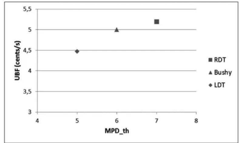
The impact ofMPD this shown in Fig. 9. The x-axis rep-resents the MPD th. The y-axis represents the UBF. Each point represents a query plan which has the highest UBF

for the given MPD th value. Again, the three formats of trees are distinguished by different symbols. For this experi-ment, theQCTEXP is fixed as 53s. We can see that when the system resources are limited (i.e., MPD this low), the left deep tree could be used to avoid the rejection of the query.

To summarize, the right deep tree is useful when the expectation of the tenant is strict, the left deep tree is neces-sary when the resources are very limited, while the bushy tree is the most benefitial in other cases. Therefore, we pro-pose to consider all these three tree formats.

4.4 Search Strategy

In this section, we first revise two types of search strategies: enumerative and randomized. Then, we propose a heuristic for solving the resource contention problem.

4.4.1 Enumerative Method

The plan enumeration method that we have revised is the one proposed in [15], which has been shown to be efficient for the generation of optimal bushy join trees. A query is represented as a connected graph with n relations R0; R1;. . .; Rn'1. The algorithm is based on the notion ofcsg-cmp-pairs, where

csg means connected subgraph andcmp is the abbreviation of complement. Suppose that, S1 is a non-empty subset of

fR0;. . .; Rn'1g, and S2 is another non-empty subset of

fR0;. . .; Rn'1g, the pair(S1, S2)is called acsg-cmp-pair, if: (1) S1 is connected, (2) S2 is connected, (3) S1\S2¼f, and (4) there exist nodesv12S1andv22S2such that there is an edge betweenv1 andv2in the query graph. The algo-rithm to efficiently list all thecsg-cmp-pairs is given in [15]. Once the csg-cmp-pairs are enumerated, the algorithm uses dynamic programming to construct the optimal bushy join tree recursively. Therefore, the method is named as DPccp

(i.e., Dynamic Programming with csg-cmp-pairs).

If we use directly theDPccp algorithm for our problem, the following pruning strategy should be applied: given two equivalent sub-plans SP1 and SP2, if UBFðSP1Þ > UBFðSP2Þ, then we can eliminate SP2.

However, this is not a valid pruning strategy in our context. Here is a counter example. For a subset fR1; R2g, we compare two sub-plans SP1¼R1fflR2 and SP2¼

R2fflR1, supposing that UBFðSP1Þ > UBFðSP2Þ. Con-sider the following two cases: (1) QCTðSP1Þ > QCT th or

MPDðSP1Þ > MPD th; (2) QCTðSP1Þ <¼QCT th and

MPDðSP1Þ <¼MPD th. For case (1), if we eliminateSP2, then no solution will be found, because the entire plan con-structed from the sub-planSP1will violate the optimization constraints. For case (2), it is not sufficient to guarantee that the entire plan constructed from SP1 will meet the con-straints, so we still cannot eliminateSP2. Therefore, in both cases, we should keepSP2.

Another pruning strategy, as used by [7], [27], is:given two equivalent sub-plans SP1 and SP2, if QCTðSP1Þ <¼

QCTðSP2Þ,MCðSP1Þ <¼MCðSP2Þ andMPDðSP1Þ <¼

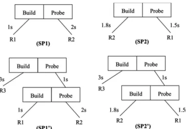
MPDðSP2Þ, we say that SP1 dominates SP2 and we eliminate SP2. Again, it is invalid in our context due to the use of the inde-pendent and pipeline parallelism. We show this by a counter example, illustrated in Fig. 10. For a subsetfR1; R2g, we take the two sub-plans SP1¼R1fflR2 and SP2¼R2fflR1. Suppose thatjR1j < jR2j. ForSP1, the operationBuildðR1Þ

takes 1s, ProbeðR2Þ takes 2s, and for SP2; BuildðR2Þ takes 1.8s,ProbeðR1Þtakes 1.5s. We haveQCTðSP1Þ ¼1þ2¼3s, and QCTðSP2Þ ¼ 1:8 þ 1:5 ¼ 3:3s. It is possible that

MPDðSP1Þ ¼2, MPDðSP2Þ ¼3, MCðSP1Þ ¼8 cents, and

MCðSP2Þ ¼10 cents. In this case, we can say thatSP1 domi-natesSP2. Now we compare an entire plan generated from

SP1which isSP10_{¼R3ffl ðR1ffl R2Þ, with the plan} gener-ated in the same way from SP2 which is SP20_¼R3ffl

ðR2ffl R1Þ. Suppose thatBuildðR3Þtakes 3s andProbeðR12Þ

takes 1s. We have QCTðSP10_{Þ ¼maxð1;3Þ þmaxð2;1Þ ¼5s} and QCTðSP20_{Þ ¼maxð1:8;3Þ þmaxð1:5;1Þ ¼4;5s, soSP1}0 does not dominateSP20_{. Thus we cannot eliminateSP2.}

Nevertheless, there exists a valid pruning strategy in our context: as said above, if QCTðSP1Þ > QCT th or

MPDðSP1Þ > MPD th, the entire plan constructed from the subplan SP1 will violate the optimization constraints. Thus,SP1can be eliminated.

In Fig. 11, we show the new enumerative algorithm using this pruning strategy, where the procedure ConstraintsMet (Plan) checks if the sub-plan meets the optimization constraints.

4.4.2 Randomized Method

We propose an extension of the Iterative Improvement (II) algorithm [24], as shown in Fig. 12. First, we randomly choose several plans as starting points. For each starting point, we check a certain number of adjacent plans. This number is a tunable parameter called “runs”. We do not check all the adjacent plans, because there could be a huge number. If no adjacent plan is found better, the current plan is consid-ered to be a local optimal plan. If an adjacent plan is better, we move to that plan and repeat the same check procedure. The number of moves is also limited by the value of the parameter runs. Finally, we compare the obtained local optimal plans and return the global optimal one.

Fig. 10. Counter example for a pruning strategy.

Fig. 11. Revised enumerative algorithm.

In the getNeighbourðÞfunction, we randomly pick a join operation in the plan, and check the following transforma-tion rules [9]:

Join commutativity: afflb¼bffla

Join associativity: (afflb)fflc¼affl(bfflc) Left join exchange: (afflb)fflc¼(afflc)fflb Right join exchange: affl(bfflc)¼bffl(afflc)

A transformation which produces a Cartesian product is considered as invalid. Among the valid transformation results, we randomly choose one.

4.4.3 Heuristic for Resource Contention

In the above algorithms, the value of the parameterMPD th

is decided by the system’s resource manager according to the current load. Assuming that, at the query optimization time, the number of available nodes in the system isnb avb, we first run the optimizer usingMPD th¼nb avb. If no solu-tion is found, it means that, there are not enough resources to run the query. In this case, we use the following heuristic: first, we run the optimizer without constraint on MPD

to find an optimal plan; then, we decide whether to execute this plan later when enough resources will be available, or suspend some other running queries to release resources, or give up the current query, according to the estimated costs.

More precisely, the heuristic includes the following steps: 1) If the optimizer cannot find a solution due to the

resource limitation, we setMPD th¼ 1and run the optimizer. Suppose that theMPDof the obtained plan isMPDopt, theQCTisQCToptand theUBFisUBFopt. 2) Rank the running queries by their completion time

in ascending order. Take the first n queries such thatPn

i¼1MPDi þnb avb >¼MPDopt. Assume that these queries are expected to finish in timet.

3) IftþQCTopt <¼QCT th, then we wait thenqueries to finish and start executing the queryQafter.

4) Otherwise, rank the running queries by their UBF

in ascending order. Take the first k queries such thatPk

i¼1MPDi þnb avb >¼MPDopt. We suspend these queries if the following condition holds:

UBFopt)t' Xk i¼1 Plti > Xk i¼1 UBFi)QCTi'Plt Qð Þ; (17)

where,Pltiis the penalty to pay if we stop the query i,

andPltðQÞis the penalty to pay if we refuse the query Q.

5) If the above condition does not hold, we reject the queryQand pay the penalty.

Note that, if there are too many query rejections, the pro-vider should consider adding new computing resources or canceling some service contracts. In this paper, we do not discuss this problem further.

5

E

XPERIMENTAL

E

VALUATION

We have implemented the cost model and the proposed search methods inside a query optimizer. Experiments have been made to evaluate the cost-effectiveness of our SLA-driven optimization approach. We have also compared dif-ferent plan search methods in terms of optimality and query

optimization cost. The latter includes optimization time and memory consumption.

5.1 Experiment Setting and Evaluated Methods For the evaluation of cost-effectiveness of our SLA-driven approach, we use a simulated multi-tenant parallel DBMS running on top of a shared-nothing architecture. Each node is composed of a 100 GIPS CPU, a 3 GB RAM, and a hard disk whose I/O bandwidth is 100 MB=s. The average disk latency is 2ms. The multi-tenant DBMS is simulated in the following way: (1) the execution of a query is simulated by using several parameters like start-time, end-time and num-ber of nodes used, (2) we assume that, at the beginning,N

queries from N different tenants arrive at the same time, and the optimizer chooses an execution plan for each query one after the other according to their session numbers. The chosen plan depends on the still available resources. Once the query plans are chosen, we assume that they start being executed in parallel at time 0, (3) when the execution of query i of tenant j is finished, the optimizer chooses a plan for queryiþ1of the same tenant under the current resource constraints. If there are enough resources, the plan starts being executed immediately. Otherwise, the execution is postponed or the query is rejected.

We compare the averageUBFof the following two meth-ods: (1) Enumerative method using the traditional approach

ENUM TRADwhich always minimizes theQCTunder the system resource constraints, and (2) Enumerative method using the cost-effective approachENUM CEMwhich maxi-mizes the UBF under the system resource constraints and the QCT threshold constraint of the SLA. To be fair, they are implemented by using the same cost model for the QCT estimation.

For the comparison of the plan search methods, we run our optimizer (implemented in JAVA) on a PC with Intel Core i5-3570 CPU 3.4 GHz, 8 GB RAM, Windows 10 (64 bits). We compare the optimality, optimization time and memory consumption of three methods: (1) ENUM CEM, (2) our proposed randomized methodRAND CEM, and (3) the Iterative-Refinement Algorithm (IRA) method proposed in [27], which adopts the Multi-Objetive Optimization (MOO) approach:IRA MOO.

The way that we do the optimality measurement of

RAND CEM is as follows: for each sample query, we run the method 100 times, calculate the averageUBF value and compare it with theUBF of the optimal plan generated by the methodENUM CEM.

5.2 Benchmark Description

We selected a subset of TPC-H [26] queries ðQ3; Q4; Q5; Q8 andQ10Þwhich represent different levels of complexity (2, 1, 5, 7 and 3 joins respectively). For each query template, we first define the SLA under the proposed negotiation framework (see Section 5.3). The scale factor that we use for the TPC-H dataset is 10. Then, we optimize the queries according to the SLA and simulate a parallel execution of queries launched simultaneously by several tenants. The workload that we use is similar to the workload for the throughput test in TPC-H benchmark. There are 3 parallel sessions which represent 3 tenants. The query sequences in these sessions are shown below:

Session 1: Q3, Q5, Q10, Q8, Q4 Session 2: Q10, Q8, Q5, Q4, Q3 Session 3: Q8, Q5, Q4, Q10, Q3

For each query, we note the start time, end time,UBFand

MPD, in order to compute the averageUBFfor the complete workload.

5.3 Defined SLA

In Table 2, we show the shortestQCTwith the correspond-ing price, the lowest price with the correspondcorrespond-ing QCT, and the expectedQCTof the tenant with the expected price. We suppose that the tolerance threshold of the tenant is 2 and the gain factor of the provider is 1. In this section, for illustration purpose, we suppose the highest selectivity for each parameter of all queries.

5.4 Cost-Effectiveness of the SLA-Driven Approach We evaluate the cost effectiveness under two different configurations. In the first configuration, we assume that the system has enough resources. In the second configu-ration, we assume that the system resources are limited, for example, there are only 16 nodes available for the workload.

5.4.1 With Enough Resources

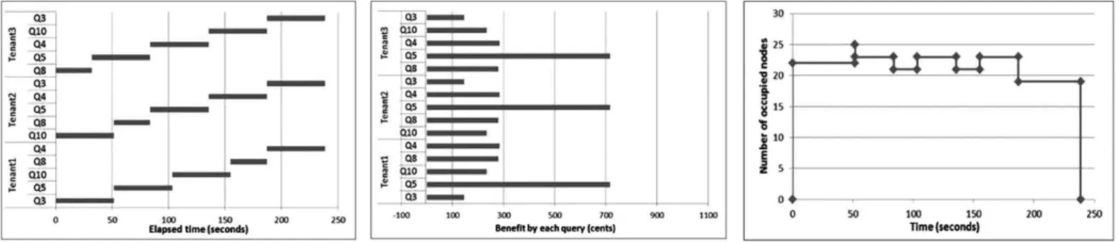
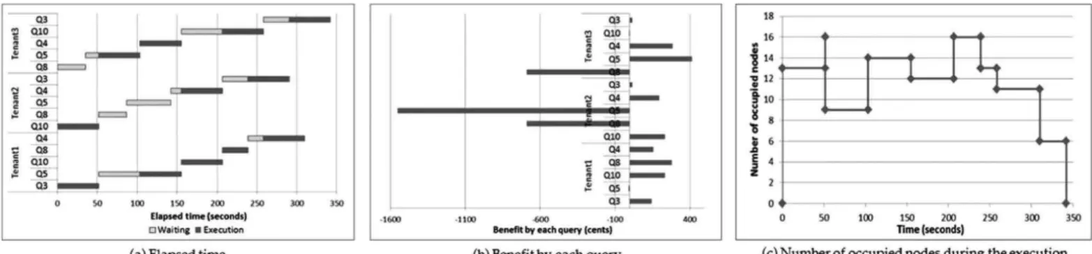
Under this configuration, a query can be processed as soon as it arrives. Fig. 13 shows the result of the ENUM_TRAD

method which always minimizes the query completion time. Fig. 13a is a Gantt chart illustrating the progress of the three sessions. They start at the same time and finish at the same time. The elapsed time is 238.8 seconds. Fig. 13b shows the benefit (i.e., revenue - cost) gained by each query. Note that, when the deadline is met, the benefit is often positively corre-lated to the price. This is normal, because a high price is usu-ally due to high resource consumption, and a high reward is deserved. The total benefit is 4407.34 cents. Fig. 13c is the number of occupied nodes at each point of time during the execution. The maximum number is 25 nodes. Based on the obtained numbers, we compute the averageUBFas follows:

UBFavg¼total benefit=elapsed time

¼4407:34=238:8¼18:46ðcents=sÞ:

Fig. 14 shows the result of our method ENUM CEM

which maximizes theUBFfor each query. We can see that, the elapsed time is 246.4 seconds, a little longer than the

ENUM TRAD method. However, the benefits of some queries are higher, and the total benefit is 5612.17 cents, 21 percent higher than ENUM TRAD. The reason is that fewer resources are consumed, as can be seen in Fig. 13c: the maximum number of occupied nodes is 18. The average

UBFis computed as follows:

UBFavg¼5612:17=246:4¼22:78ðcents=sÞ:

5.4.2 With Limited Resources

We assume that there are only 16 nodes available for the workload. When a query arrives, if there are not enough resources, it cannot be processed until some other queries

TABLE 2 Defined SLA QCTs (s) PRs (cents) QCTL (s) PRL (cents) QCT exp (s) PR exp (cents) Q3 51.6 459 55.2 370 55 375 Q4 51.7 569 51.7 569 55 569 Q5 51.7 1672 72.5 925 55 1553 Q8 32.1 821 55.3 689 55 691 Q10 51.7 563 59.1 457 55 516

Fig. 14. MethodENUM CEMwith enough resources. Fig. 13. MethodENUM TRADwith enough resources.

finish. Fig. 15 shows the result ofENUM TRAD. In Fig. 15a, we see that some queries have to wait due to resource limita-tion, and some others have to be rejected because the SLA cannot be met. For example, the first queryQ8of tenant 3 and two queries of tenant 2 have been rejected. The second query of tenant 3 waited 16.6 seconds. Therefore, the total elapsed time is longer (342 seconds). The benefits for some queries are negative, for example,Q5of tenant 1,Q5andQ8of tenant 2, etc. The total benefit is -1162.42 cents, as shown in Fig. 15b. Fig. 15c shows the number of occupied nodes at each point of time during the execution. The averageUBFis negative:

UBFavg¼ '1162:42=342¼ '3:4ðcents=sÞ:

The result of our method ENUM CEM can be found in Fig. 16. The total elapsed time is 294 seconds, and the total benefit is 4892.59 cents. So the averageUBFis:

UBFavg¼4892:59=294¼16:64ðcents=sÞ:

5.4.3 Summary

With enough resources, theENUM TRAD method spends very little time to finish the queries, but its economic cost is rather high, so the benefit is low. Our methodENUM CEM

has a better trade-off between the query completion time and the economic cost, so the overall benefit is higher.

With limited resources, both methods need more time to finish the queries, because some queries have to wait for resources to be released. In addition, some queries may be rejected. This situation happens less frequently for

ENUM CEM, so its total elapsed time is shorter than that of

ENUM TRAD. The averageUBFofENUM CEMis always higher due to the SLA-driven cost-effective optimization problem definition.

The experimental results are summarized in Table 3. We can conclude that, under both configurations, our method is more cost-effective than the method ENUM TRAD. With enough resources,ENUM CEMgains 23 percent more than ENUM TRAD. With limited resources, ENUM CEM

still gains, but ENUM TRAD starts losing due to query rejections.

5.5 Comparison of the Plan Search Methods

The RAND CEM method does not enumerate all possible execution plans, so the optimal plan may be skipped by the search algorithm. As for the method IRA MOO, since its pruning strategy is not valid when parallel execution is conci-dered, as demonstrated in Section 4.4.1, the optimal plan may be eliminated in an early stage. When a sub-optimal plan is

Fig. 15. MethodENUM TRADwith limited resources.

Fig. 16. MethodENUM CEMwith limited resources.

TABLE 3 Overview of the Results

With enough resources With limited resources

ENUM_TRAD ENUM_CEM ENUM_TRAD ENUM_CEM

Total elapsed time (seconds) 238.8 246.4 342 294

Total benefit (cents) 4407.34 5612.17 '1162.42 4892.59

proposed, the UBF becomes lower. Therefore, we compare the optimality ofRAND CEMandIRA MOOwith the exact methodENUM CEM. For RAND CEM, we run 100 times the method for each query template and compute the average

UBF, in order to measure the long term consequence on the

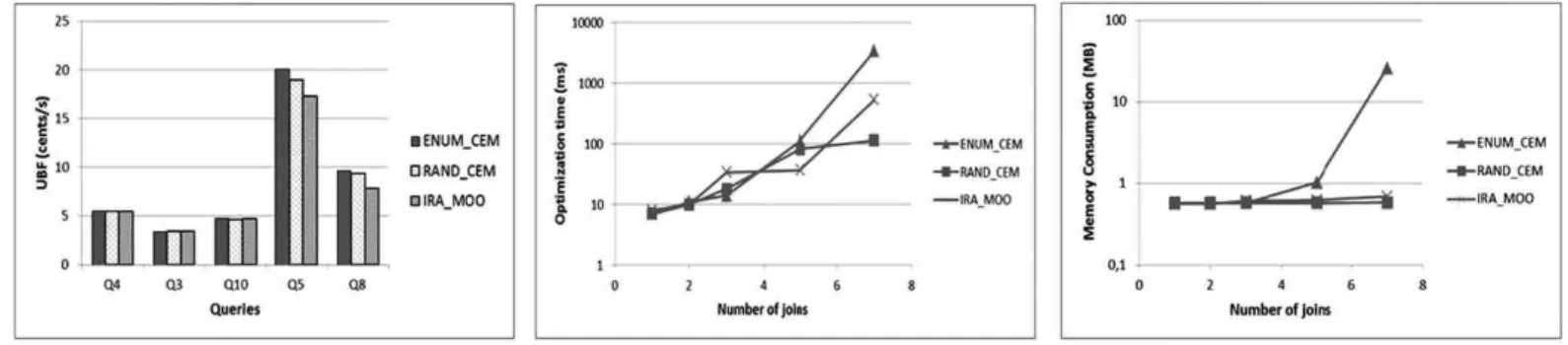
UBF. In this experiment, we assume that there are enough resources. The result is shown in Fig. 17a. We can see that, compared to the optimal UBF, the degradation of

RAND CEM is no more than 6 percent, while the degrada-tion ofIRA MOOcan reach 19 percent. Note that the value of runs ofRAND CEMfor each query template has been tuned to make the result close to optimal. The approximation factor ofIRA MOOis 1.15 which was shown to be a good trade-off between the optimiality and the optimization cost in [27].

For fairness, based on the same setting, we measure the optimization time and memory consumption for the exam-ple queries and compare the three methods. The optimiza-tion time is shown in Fig. 17b and the memory consumpoptimiza-tion is shown in Fig. 17c. With theENUM CEM, both the opti-mization time and the memory consumption become very high when there are 7 joins. Even though some plans can be eliminated by the pruning strategy, the number of gener-ated plans is still proportional to the total number of possi-ble plans, which grows exponentially with regard to the number of joins [25]. With the RAND CEM method, the optimization time also grows when there are more joins, because the number of runs should be increased to find a near optimal plan. However, it is always much more efficient than theENUM CEM method. As for the memory consumption of the RAND CEM method, it is almost a constant. The IRA MOO method is often less expensive thanENUM CEM, but more costly thanRAND CEM.

Despite the expensive optimization cost, we believe that in some situations, the ENUM CEM method could be more advantageous than the other methods. For example: (1) when there are less than 7 joins, all methods have equivalent optimization costs, but theENUM CEMmethod guarantees the optimality; (2) when the QCTEXP is very large due to the huge size of the database, the optimization time of theENUM CEM method becomes relatively small compared to the query execution time thus can be ignored; (3) when the QCTEXP is very close to the QCTS, or the

MPD th is very close to the minimum value of MPD, theENUM CEMmethod could eliminate many intermedi-ate sub-plans thus becomes very efficient. On the other hand, the RAND CEM and IRA MOOmethods will have a high risk of not being able to find the optimal plan.

6

C

ONCLUSION AND

F

UTURE

W

ORK

In this paper, we first proposed a SLA negotiation frame-work such that a tenant could define the performance objec-tive together with the provider. The tenant does not have to know the query execution detail, but he should not worry about being cheated, because he can compare offers from different providers and choose the best one. As for the pro-vider, the offer that he proposes is based on its own estima-tion, so the performance objective is achievable and the benefit could be maximized by using appropriate techni-ques. For this purpose, we then formally defined the cost-effective query optimization problem. We included the eco-nomic cost and benefit into our cost model. We explored a large search space with different tree formats. We revised an enumerative search method and a randomized search method to make the optimization more efficient.

Experimental results show that: (1) our optimization methodENUM CEM is much more cost-effective than the

ENUM TRAD method which always minimizes the query completion time (e.g., more than 23 percent); (2) for our optimization problem, the enumerative search method

ENUM CEMmay become prohibitive when there are more than 6 joins, while the randomized search method

RAND CEM has reasonable query optimization time and memory consumption, and it is superior in all aspects to a related work IRA MOO; (3) however, the ENUM CEM

method can be a good choice in some special cases.

In the future, we will include the aggregation operators into our cost model. After that, as previously said, a further research direction could be adapting robust query optimiza-tion methods [28] to the cloud context, in order to minimize the renegotiation risk.

R

EFERENCES

[1] Z. Abedjan, L. Golab, and F. Naumann, “Profiling relational data: A survey,”VLDB J., vol. 24, no. 4, pp. 557–581, Aug. 2015. [2] Amazon RDS. (2018). [Online]. Available: https://aws.amazon.

com/rds/

[3] Amazon RDS Service Level Agreement. (2016, Mar.). [Online]. Available: https://aws.amazon.com/rds/sla/.

[4] S. Chu, M. Balazinska, and D. Suciu, “From theory to practice: efficient join query evaluation in a parallel database system,” in

Proc. ACM SIGMOD Int. Conf., May 31-Jun. 4, 2015, pp. 63–78. [5] G. Copeland, W. Alexander, E. Boughter, and T. Keller, “Data

placement in bubba,” inProc. ACM SIGMOD Int. Conf., Jun. 1-3, 1988, pp. 99–108.

[6] S. Das, V. R. Narasayya, F. Li, and M. Syamala, “CPU sharing techniques for performance isolation in multitenant relational database-as-a-service,” Proc. VLDB Endowment, vol. 7, no. 1, pp. 37–48, Sep. 2013.

[7] S. Ganguly, W. Hasan, and R. Krishnamurthy, “Query optimiza-tion for parallel execuoptimiza-tion,” inProc. ACM SIGMOD Int. Conf., Jun. 2-5, 1992, pp. 9–18.

[8] Y. E. Ioannidis and E. Wong, “Query optimization by simulated annealing,” in Proc. ACM SIGMOD Int. Conf., May 27-29, 1987, pp. 9–22.

[9] Y. E. Ioannidis and Y. C. Kang, “Randomized algorithms for opti-mizing large join queries,” in Proc. ACM SIGMOD Int. Conf., May 23-25, 1990, pp. 312–321.

[10] Y. E. Ioannidis and Y. C. Kang, “Left-deep vs. bushy trees: An analysis of strategy spaces and its implications for query opti-mization,” in Proc. ACM SIGMOD Int. Conf., May 29-31, 1991, pp. 168–177.

[11] M. Kitsuregawa, H. Tanaka, and T. Motooka, “Application of hash to database machine and its architecture,” New Genenation Comput., vol. 1, no. 1, 1983, pp. 66–74.

[12] H. Kllapi, E. Sitaridi, M. M. Tsangaris, and Y. Ioannidis, “Schedule optimization for data processing flows on the cloud,” in Proc. ACM SIGMOD Int. Conf., Jun. 12-16, 2011, pp. 289–300.

[13] W. Lang, S. Shankar, J. M. Patel, and A. Kalhan, “Towards multi-tenant performance SLOs,” inProc. IEEE 28th Int. Conf. Data Eng., Apr. 1-5, 2012, pp. 702–713.

[14] M. V. Mannino, P. Chu, and T. Sager, “Statistical profile estima-tion in database systems,” ACM Comput. Surv., vol. 20, no. 3, pp. 191–221, Sep. 1988.

[15] G. Moerkotte and T. Neumann, “Analysis of two existing and one new dynamic programming algorithm for the generation of optimal bushy join trees without cross products,” in Proc. 32nd Int. Conf. Very Large Data Bases, Sep. 12-15, 2006, pp. 930–941. [16] V. R. Narasayya, S. Das, M. Syamala, B. Chandramouli, and

S. Chaudhuri, “SQLVM: Performance isolation in multi-tenant relational database-as-a-service,” inProc. 7th Biennial Conf. Innova-tive Data Syst. Res., Jan. 6-9, 2013, Online Proceedings, [Online]. Available: www.cidrdb.org.

[17] Oracle Data Cloud. (2018). [Online]. Available: https://cloud. oracle.com/en_US/data-cloud.

[18] Oracle Cloud Enterprise Hosting and Delivery Policies. Version 2.4. (2017, Dec.). [Online]. Available: http://www.oracle.com/us/ corporate/contracts/ocloud-hosting-delivery-policies-3089853.pdf. [19] J. Ortiz, V. T. de Almeida, and M. Balazinska, “Changing the face

of database cloud services with personalized service level agreements,”. inProc. 7th Biennial Conf. Innovative Data Syst. Res., Jan. 4-7, 2015, Online Proceedings, [Online]. Available: www. cidrdb.org.

[20] D.A. Schneider, and D. J. DeWitt, “Tradeoffs in processing complex join queries via hashing in multiprocessor database machines,” in Proc. 16th Int. Conf. Very Large Data Bases, 1990, pp. 469–480.

[21] P. G. Selinger, M. M. Astrahan, D. D. Chamberlin, R. A. Lorie, and T. G. Price, “Access path selection in a relational database man-agement system,” inProc. ACM SIGMOD Int. Conf., May 30-Jun. 1, 1979, pp. 23–34.

[22] SLA for Azure SQL Database. (2015, May). [Online]. Available: https://azure.microsoft.com/en-us/support/legal/sla/sql-database/v1_0/.

[23] SQL Azure. (2018). [Online]. Available: https://azure.microsoft. com.

[24] A. N. Swami and A. Gupta, “Optimization of large join queries,” inProc. ACM SIGMOD Int. Conf., Jun. 1-3, 1988, pp. 8–17.

[25] K. L. Tan and H. Lu, “A note on the strategy space of multiway join query optimization problem in parallel systems,” ACM SIGMOD Record, vol. 20, no. 4, pp. 81–82, Dec. 1991.

[26] TPC-H Benchmark, Version 2.17.3, Transaction Processing Perfor-mance Council. (2017, Apr.). [Online]. Available: http://www. tpc.org/tpch/.

[27] I. Trummer and C. Koch, “Approximation schemes for many-objective query optimization,” inProc. ACM SIGMOD Int. Conf., Jun. 22-27, 2014, pp. 1299–1310.

[28] S. Yin, A. Hameurlain and F. Morvan, “Robust query optimization methods with respect to estimation errors: A survey,” ACM SIGMOD Record, vol. 44, no. 3, Sep. 2015, pp. 25–36.

Shaoyi Yin received the PhD degree from the University of Versailles, France, under an INRIA doctoral contract and defended in June 2011. Since September 2012, she has worked with Paul Sabat-ier University, in the Pyramid team of the IRIT Labo-ratory, as an associate professor. Her current research interests mainly include query optimiza-tion in parallel and large-scale distributed environ-ments, especially in the cloud environment.

Abdelkader Hameurlain is a full professor in computer science with Paul Sabatier University (IRIT Lab.) Toulouse, France. His current research interests include query optimization in parallel and large-scale distributed environments, and mobile databases. He has been the general chair of the International Conference on Database and Expert Systems Applications (DEXA’02, DEXA’11, and DEXA’17). He is a co-editor in chief of the Interna-tional Journal on Transactions on Large-Scale Data- and Knowledge-Centered Systems(LNCS, Springer).

Franck Morvan received the PhD degree in computer science from Paul Sabatier University, France, in 1994. He worked with Dassault Data Services Society. He is currently a full professor with Paul Sabatier University, Toulouse, France, and a member of the IRIT laboratory. His main research interests include query optimisation in distributed and parallel databases, mobile agents, and mobile computing.