Characteristics and Implications for Carriers’ Operations and
Data Collection Efforts
Miguel Andres Figliozzi*
Lynsey Kingdon
Andrea Wilkitzki
The University of Sydney
The Institute of Transport and Logistics Studies Faculty of Economics & Business
Sydney, NSW 2006 *corresponding author [email protected]
August 1, 2006
Number of words: 4980 + 2500FREIGHT DISTRIBUTION TOURS IN CONGESTED URBAN AREAS: CHARACTERISTICS AND IMPLICATIONS FOR CARRIERS’ OPERA TIONS AND DATA COLLECTION EFFORTS
Miguel Andres Figliozzi Lynsey Kingdon Andrea Wilkitzki
ABSTRACT
This research analyses several months of truck activity records in an urban area. Data corresponds to the daily activity of less than truckload (LTL) delivery tours in the city of Sydney. The analysis of the data provides insightful information about urban truck tours and congestion levels. Route patterns were identifie d and their relationship to trip and tour length distribution was analyzed. Travel between different industrial suburbs explains the shape of multimodal trip length distributions. Variations in daily demand explain the normal-like shape of the tour trip d istribution. Tour data indicate that there is no clear relationship between tour distance, percentage of empty trips, and percentage of empty distance. Congestion costs and operational implications are discussed as well as truck driver perceptions regarding congestion and route choice. It is argued that large metropolitan areas should offer open internet access to congestion data and vehicle routing tools in order to reduce unnecessary buffers in route design and to reduce the amount of truck kilometers traveled.
KEYWORDS: Freight Transportation, Urban Freight Demand, Carrier Behavior, Shipper Behavior, Truck Traffic, City Logistics, Truck Tours, Congestion, Truck Trip Distribution, Freight Data Collection, Truck Tours , Empty Trips
1. Introduction
Unlike the case of urban passenger surveys and models, urban freight data sources and models of behavior are mostly of an aggregated nature. Urban freight data needed for disaggregate models that predict trip generation, distribution, or network assignment are scant or nonexistent [1]. Confidentiality issues are usually an insurmountable barrier that precludes the collection of detailed and complete freight data. Understandably, companies are unwilling to disclose any type of information that may be used by competitors or that may infringe customers’ rights regarding privacy, proprietary data, or security.
The lack of detailed or complete data sources is strikingly evident regarding urban truck tours or trip chains . A recent study of 13 American cities indicates that a predominant share of freight trips that contribute to freight vehicle kilometers traveled (VKT) originate at distribution centers (DC) or warehouses [2]. Trips that originate at distribution centers (DC) warehouses are tours or trip chains that usually involve more than 2 stops. Due to data limitations and availability, truck tours are largely ignored in traditional four-stage transportation modeling approaches borrowed from the passenger modeling literature or in most urban freight models. A recent and comprehensive survey of urban freight modeling efforts across nine industrialized countries of America, Europe, Oceania, and Asia1 confirms the absence of urban truck tour analytical models [3].
Congestion is a common phenomenon in all major cities of the world. The uncertainty brought by congestion impacts the efficiency of logistics operations. Direct and indirect costs incurred due to congestion have been widely studied and reported, mostly in relation to passengers’ value of travel time, carriers’ value of t ravel time and shippers’ market access costs, logistics costs, production costs, and productivity costs [4]. However, the specific operational and data collection implications of congestion for truck tours have not been discussed in the literature.
This research contributes to the understanding of truck tours by analyzing tour and congestion related data at a disaggregate le vel. The authors had access to detailed truck run sheets where the daily activities of trucks were recorded. The contributions of this research are threefold: a) presents novel insights and data analysis about urban truck tours, empty trips, and empty distances, b) furthering the discussion of congestion costs from a carrier’s perspective, and c) suggesting new ways to disseminate congestion data to improve the efficiency of carriers’ routing in urban areas.
The research is organized as follows: section two provides a literature review of truck tours and congestion costs. Section three describes the data sources used in this research. Section four analyzes tour characteristics such as trip and tour length distributions. Section fivedescribes the challenges posed by the analysis of congestion levels and the results obtained regarding congestion. Section six discusses congestion costs and operational implications of delays from a carrier’s perspective. Section seven analyze s the driver’s perception of congestion levels. Section eight discusses the need for online public sources of congestion and truck routing tools. Section nine ends with conclusions.
1
2. Literature Review
Ogden [5] breaks down the data collection needs for urban freight modeling into five distinct themes: vehicle fleet, vehicle flows, commodity flows, major freight generators, and major freight corridors. The data collection needs described by Ogden mostly apply to aggregated fleet and flows data. However, it is increasingly recognized that aggregated urban freight data is highly valuable in describing the state of the system but it is insufficient to forecast or analyze policy/network changes. In particular, information regarding truck tours is lost in the aggregated data flows.
Incipient work regarding truck tour data collection and modeling has recently begun. Data collection efforts that aim to capture the complex logistical relationships of commercial tours have been undertaken in Canada [6], USA [7], and the Netherlands [8]. In the modeling arena, and to the best of the author’s knowledge, if truck tours are included in models the tours are simulated. The tour simulation can combine a tour optimization embedded in a dynamic traffic simulation environment [9] or the simulation can be combined with discrete choice modeling [6]. In the latter, tour stops (number, purpose, location, and duration) are modeled using regression and logit models and then micro -simulated. To the best of the author’s knowledge, the only research that attempts to study properties of urban tours analytically was performed by Figliozzi [10]. This work classifies tours according to the commercial activity that generates the tour and routing constraints faced by the carriers
Tour data from different cities indicate that the average number of stops per tour is significantly higher than one or two stops. The city of Calgary reports approximately 6 stops per tour [11], Denver reports 5.6 [7] and data from Amsterdam indicate 6.2 stops per tour [8]. In the case of Denver, approximately 50% of single and combination truck tours include 5 to 23 stops per tour. Data from Amsterdam indicate that the amount of time that is taken during unloading/loading stops is 21 minutes on average (mode 10 min.) and that the average time to reach the service/delivery area is 25 minutes (mode 10 min.). The data suggest a skewed distribution which may be due to the impact of congestion and delays at stops.
There is a large body of literature on the impacts of congestion in urban areas [4]. However, the impact of congestion at the company or disaggregate level is not common. A noteworthy exception is the study performed by Sankaran et al. [12] regarding congestion levels and replenishment order sizes in Auckland, New Zealand. According to Sankaran et al.’s study, it was estimated that congestion may increas e the ship-to-factory cost by roughly 5–10% and may increase distribution costs from the factory to distribution outlets and building sites by roughly 10–15%. Certain types of logistics operations aggravate the negative effects of congestion such as just-in-time (JIT) deliveries with inflexible distribution contracts (e.g. time-definite delivery requirements).
3. Data Sources and Collection
The analysis presented in this research is based on truck routing data provided by a freight forwarding company based in Botany Bay, Sydney, Australia. Botany Bay is an ideal location for a freight forwarding or distribution company due to its proximity to both the port of Sydney as well as the international airport. In addition, downtown
Sydney is at a relative close distance, approximately 12 kilometers. Due to its strategic location, Botany Bay is the preferred location of many transport related industries and activities.
Congestion is an important issue within the Sydney area. According to Australian Bureau of Transport Economics [13], the costs of congestion in Sydney area was six billion Australian dollars in 1995 and will reach nine billion Australian dollars by 2015 . Several approaches to handle this problem within the Sydney area are being analyzed, ranging from road improvements to road pricing. Due to the high concerns regarding the future of congestion in Sydney and its implications for freight carriers, a research report was conducted to analyze congestion in the Sydney area. Access to detailed routing data is always difficult due to privacy concerns. Exceptionally, this was not an issue in this research because one of the research team members was at the time a student in the Masters of Logistics program at the University of Sydney and in a working relationship with a freight forwarding company. Ready access was allowed not only to truck daily activity sheets but also to interview the corresponding truck driver.
The routing data presented in this paper was extracted from truck activity sheets over an eight-month period, between September 2005 and April 2006. The data corresponds to the routes of a twelve-ton truck, which is driven by a driver with 35 years of working experience in the Sydney metropolitan region. The truck driver was interviewed to check for data consistency and perceptions about congestion.
Most pick-up trips are from the port terminals to the depot. Distribution is concentrated in the Botany area itself and to industrial suburbs of Sydney, such as Bankstown, Kingsgrove, Milperra, Silverwater, and Smithfield. One-way trips in the Botany area have a length in the range of 1 to 5 kilometers from the depot. One-way connecting trip between the depot and other industrial suburbs are substantially longer, usually ranging between 14 to 40 kilometers to/from the depot. Local trips within the industrial suburbs, for example connecting two customers in Silverwater, are roughly comparable in length to the local trips within Botany. Figure 10 shows the location of the Port of Sydney and the mentioned industrial suburbs.
Truck deliveries were less than truckload (LTL) to companies in the retailing, service, and manufacturing sectors. In the eight-month period the truck served 190 different customers, however, the top 20% of delivery locations account for 71.2% of the total number of deliveries/stops during the eight -month period. Each daily route and sequence of customers differed depending on what freight was available on a particular day for collection and/or delivery. However, most routes followed one of these patterns: a) distribution in the Botany area, b) distribution in an industrial suburb after traveling a connecting distance from the depot/Botany area, or c) a combination of a) and b) patterns.
4. Tour Characteristics
In this research, an urban tour is defined as the closed path that a truck follows since it leaves its depot and visits different destinations (two or more customer destination or stops) in a sequence before returning to the depot during a single driver shift. Therefore , a tour is comprised of several trips; a trip is defined by the distance or time traveled between two consecutive stops.
An individual truck tour usually amounts to less than 300 kms from the depot since they are restricted by the average travel speed, loading/unloading time, number of stops, and number of working hours in a shift. USA data
estimates that warehouse delivery vehicles have an average of 105 kms (approximately 65 miles) per day per vehicle [14]. The value obtained as an average for the USA is very close to the values obtained for the study in Sydney.
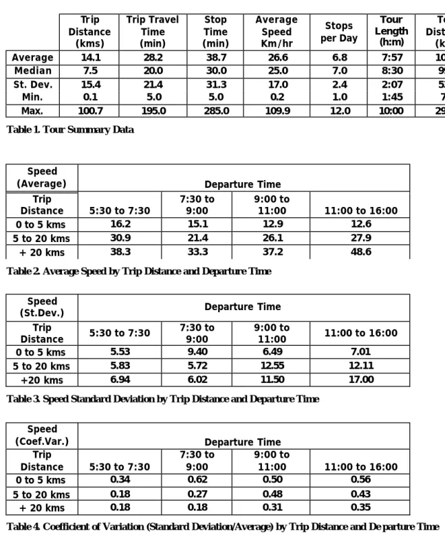
Using the collected data from Sydney, see Table 1, a “typical” or median tour can be defined as a tour of approximately 100 kilometers. The vehicle spends 4 hours on the streets at an average speed of 25 km/h and spends 3.5 hours stopped (loading/unloading, paperwork, refueling, etc.). In such a tour, assuming ½ hour for the driver lunch break, the length of the tour is 8 hours. Approximately 44% of the tour time is spent at customer locations (loading/unloading, paperwork, etc.) and 50% of the tour time is spent driving to or between customers. The remaining 6% corresponds to the driver’s lunch time or personal needs , refueling, etc.
Table 1 indicates that although the average and median tour length are fairly close to a working shift of 8 hours, variations in daily demands may render tours as short as 1 hour and 45 minutes or as long as 10 and a half hours. Stop duration time at customer stops is shown to vary widely between 5 minutes and a maximum of 285 minutes. Although the variation of stop time is significant, most of the variation can be s atisfactorily explained when accounting for customer, type of product, delivery quantity, and type of loading/unloading facilities. Shortening the duration of customer stops can greatly improved the efficiency of truck tours as discussed in [10].
As mentioned in literature review, tour data from different cities indicate that the average number of stops per tour is significantly higher than two stops. The city of Calgary reports approximately 6 stops per tour [11], Denver reports 5.6 [7] and data from Amsterdam indicate 6.2 stops per tour [8]. The data from Sydney reports an average number of 6.8 stops and a median value of 7 stops per tour which is comparable to previous studies.
a. Trip and Tour Length Distribution
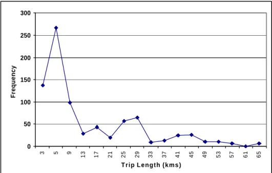
As indicated in Figure 1, the trip length distribution shows a clear peak between 2 and 9 kilometers. This is explained by the short trips in the Botany area and the local deliveries in other industrial areas. A second peak is found between 21 and 33 kilometers. The second peak is caused by trips to/from industrial suburbs (connecting trips between the depot and distribution areas). For example, it may take a trip of 27 kilometers to arrive to the Silverwater distribution area. This 27 kilometer trip may be followed by shorter local trips, from 2 to 9 kilometers, in the Silverwater area.
It is clear that the relative location of major freight generators (i.e. large factories, distribution areas, intermodal facilities, etc.) in relation to their service areas affect the shape of the trip length distributions. Empirical observations confirm that multimodal trip length distributions are found in practice as indicated by Holguin-Veras and Thorson [15] using aggregated data for Guatemala City. Their observations are con firmed by our results using disaggregated data. The average distance between stops and the average number of stops per tour is likely to be related to the dispersion of the trip length distribution around the modal points as discussed in a later section.
The gravity model is a popular technique to model trip distribution. This model is usually calibrated by comparing the trip length distribution (TLD) and trip length averages in the model against the observed trip length distribution and average. In order to calibrate gravity models it is typically assumed that there is a decrease in the number of trips as distance or time between origins and destinations increases, i.e. a unimodal impedance function. However, if the magnitudes of the connection distance and the average distance between stops are significantly different,
a unimodal impedance function may not be able to adequately represent the distribution of trip lengths [15]. As shown in Figure 1, the location of industrial suburbs can significantly alter the shape of the TLD.
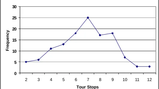
Tour length distribution is significantly different from the distributions of trip-length and number of stops per tour. . As shown in Figure 2, the tour length distribution resembles a normal or log-normal shape. This is not surprising since the tour length distribution reflects variations in daily number of customer demand and locations. The distribution of tour lengths and the number of stops per tour do not follow the same pattern as shown in Figure 3. This is explained by the existence of long tours with few stops in a distant suburb and a short tour with many stops in a near suburb.
b. Tour Length and Percentage of Empty Trips and Distance
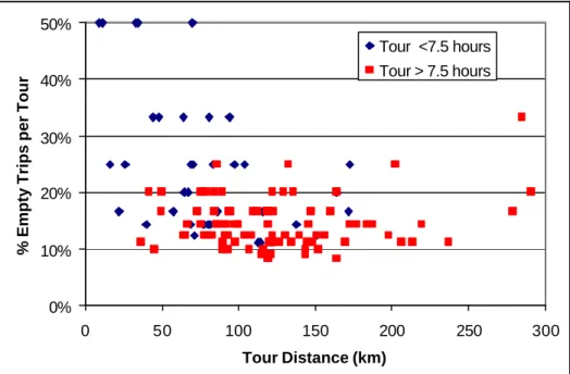
As indicated in Figure 4 and 5, there is not a clear relationship between tour length and percentage of empty trips or empty distance per tour. Furthermore, there is no clear relationship between percentage of empty trips per tour and percentage of empty distance per tour even after accounting per tour duration. The percentage of empty trips per tour cannot exceed 50% and decreases as the number of customers visited per tour increases; the last leg or trip of the tour is the empty return to the depot. However, it is possible to have a percentage of empty distance per tour that exceeds 50%. This is possible in a delivery tour where the last stop is the farthest point in the tour from the depot. After the deliveries are completed the driver may take a longer route to return to the depot to avoid toll routes. Hence, it is possible in the same tour to have 62% of empty traveled distance and just 20% percentage of empty trips (with four customers ). The percentages would be even more dissimilar if the tour had more stops. Therefore, the percentage of empty trips per tour in an urban area can be a very poor indicator of the percentage of empty distance traveled by distribution trucks.
5. Congestion Level and Tour Speed Analysis
From the daily truck activity records, travel times were estimated as the difference between departure and arrival times. Distances between origin and destination addresses were calculated using a Sydney street network. The average speed between origin and destinations was estimated using the travel time and distance between addresses. By filtering the data obtained from the driver run sheets, delivery points and links occurring frequently were identified.
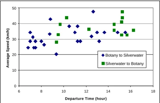
Figure 7 represents the speed observations for the connecting link between the Depot and the suburb of Silverwater. In the figure it is possible to observe that the speed in the 7:30 -8:30am period tends to be lower than during the rest of the day. During the morning rush hour the average speed is 26.2 kilo meters per hour (km/h) while speed average for the full day is 32.2 km/h. Figure 7 also shows that directional effects can be important, with return trips from Silverwater to Botany having a higher average speed than trips from Botany to Silverwater.
Despite the use of several months of complete routing data, congestion analysis proved to be a difficult task. Five factors that complicated analysis are mentioned:
(a)The sheer number of possible origin destination (OD) pairs. As 190 customers were visited, the possible number of network links between customers is 17,955.
(c)Departure time vs. arrival t ime: long trips may fall in both rush and non-peak periods. For example, a trip that started at 8:30 am during the rush hour period and finished at 11:30 am during the non-rush hour period. (d)Directional effects : morning and evening rush hours can have different impacts whether heavy traffic is moving
towards downtown or not.
(e)No information available about potential travel times in alternative routes
(f) At the tour level, variation of customer demands precludes the direct comparison of tours travel times. Tours may take place in the same suburbs but the variation of the daily number of stops, location and delivery size make each tour almost unique.
To analyze the effects of congestion on travel speed, the data was aggregated by trip length and time of day. The trip lengths of 5 and 20 kilometers correspond to those points on the trip distribution chart that separate local trips from long connecting trips between suburbs (see Figure 1).
Table 2 shows the speed average arranged by trip distance and time of the day. It is observed that short trips have the lowest travel speed; long trips have the highest travel speed. This can be explained by the type of streets and highways used by short and long trips. Short trips take place mostly on local streets; long trips are more likely to use freeways or primary highways. In all cases, the average speed decreases from the early morning period (trip departure before 7:30am) to the morning peak hour period (trip departure between 7:30-9:00am). The average speed recovers after 9:00 am for medium and long trips. The average speed does not recover for short trip s. In the driver’s opinion, a constant congestion was found in the Port Botany-Botany areas where the traffic levels are higher since this area holds most of the infrastructure used for the international forwarding industry.
Table 3 shows the speed standard deviation arranged by trip distance and time of the day. It is observed that the speed standard deviation is lower during the congestion period than after 9:00 am. The data suggests that even though the speed travel time is lower during the rush hour it is nonetheless subject to less variation. Table 4 shows the coefficient of variation, ratio between standard deviation and average, arranged by trip distance and time of the day. Short trips have the largest coefficient of variation in all cases. One e xplanation for this is the larger variation in the type of local areas traveled by short trips. Part of the variation can also be attributed to the driver’s tendency to round arrival or departure times to five minute intervals. This rounding has a higher impact on short distance trips than for longer distances.
The relationships between trip length and speed shown in Table 2 can be extended to the relationship between tour length and average tour speed as shown in Figure 8; long trips are more likely to use freeways or primary highways and therefore have a higher travel speed. An interesting relationship between tour time spent at customer stops and the ratio between tour distance and tour stops is shown in Figure 9. On the upper left section of the graph , tours with many stops spend a high percentage of the tour time at the customers’ sites; a feasible tour can be finished within normal working hours (no overtime) if the average distance between stops is short. On the lower right section of the graph, tours with few stops and long trips spend a low percentage of the tour time at the customers’ sites; with few stops, a feasible tour can be finished within normal working hours even if the average trip length is longer. Thus, the variation in tour length cannot be explained solely based on the variation of the number of stops, see Figure 3. This is because the
distance between the suburb and the depot may take a high percentage of the total tour distance, the number of feasible stops per tour decreases as the distance between distribution suburbs and the depot increases. Therefore, congestion and delays may have a higher impact on distant distribution suburbs.
As tours are constrained by their duration and time delivery constraints , there is a tradeoff between serving a small number of customers in a distant suburb and serving a large number of customers located at a short distance from the depot. The final route design takes into account the daily demand realization and the best split of customers among available vehicle capacities. The daily route patterns are then a combination of tours with distribution in the local depot area, with distribution in another industrial suburb, or a combination of the two. Next section discusses how congestion affects route design and the implementation of route plans.
6. Discussion -- congestion c osts and operational i mplications
Carriers and distributors in urban areas are faced with the daily design of pick-up and delivery routes. As discussed in Section 5 large amounts of travel speed observations by OD pairs, time of the day, and direction of travel are needed. Even with aggregated congestion data sophisticated algorithms and vehicle routing software are needed to take into account congestion and travel time uncertainties.
The use of Advanced Traveler Information Systems (ATIS) and affordable GPS tracking and reporting devices by truck drivers can decrease the effects of congestion [16, 17]. The design and dynamic control of vehicle routes requires the formulation of a dynamic vehicle routing problem with time dependent travel times [18]. In order to apply this type of methodology, a real-time vehicle control is necessary as well as real-time information about congested areas. Congestion costs related to routing can be classified as overhead and operational costs. Overhead costs are associated with the acquis ition and maintenance of congestion and travel time data. Overhead costs may also include routing software and communication equipment as well as related employee hours to operate the system. Operational costs are related to the handling of delays. A carrier facing route delays may opt to: (a) pay drivers ’ overtime in order to complete the route, (b) reschedule non-priority or non-time sensitive deliveries for the next day, and (c) divert or alter the route(s) to minimize costly delays. All these options come at a price, either paying overtime, loss of customer goodwill, or longer routes and higher operation costs. In addition, employee time to handle customer service and rescheduling issues should also be considered an operational cost. Although significant, these overhead and operational costs are not readily estimated at an aggregated level. To the best of our knowledge, they are not included in any congestion costs studies.
Despite the availability of real time information and sophisticated vehicle routing and tracking software, there are routing decisions that must be taken at the outset of the working day such as the assignment of vehicles to customers. High congestion may lead to more buffers in the logistics pipeline. Carriers assign fewer customers per vehicle in order to cope with travel time uncertainties or speed reductions due to traffic congestion. In particular, with time definite deliveries or close of business delivery deadlines it is not possible to compensate delays with overtime working hours. JIT penalties or loss of customer goodwill due to late deliveries is usually high enough to justify buffers in the route design.
Truck drivers experience congestion on a daily basis. Next section describes a truck driver’s perception of congestion in the Sydney area.
7. Driver’s perception of congestion
We conducted an interview with the driver of the truck to check for data consistency purposes and to get a hint of the driver’s perception of traveling times and congestion. This driver has 35 years working experience driving within the Sydney metropolitan area. In this particular company, d rivers have a highly influential role in the design of routes .
Part of the interview consisted of taking a day’s demands and comparing the solution obtained with routing software with the routes effectively implemented on that given day. Questions were asked regarding: (a) congestion as a contributing factor to the choice of route, (b) if congestion affects the departure time, and (c) delivery order to minimize congestion problems. In general, the driver’s route usually matched the solution that could be obtained from a visual solution of the routing problem. An important issue was the direction of route travel, e.g. clockwise or counterclockwise. This is a key point since the direction determines what route or link is used to return to the depot in the afternoon/evening or if local deliveries should be completed before traveling to other suburbs or after completing deliveries in other suburbs. Not surprisingly, contradictions with the data collected regarding variations in travel speed did arise. It is an open research question how truck drivers compare and evaluate routes. As shown in Tables 2, 3 and 4 there are many cases of trade-offs between average travel speed and travel speed variability. The correct choices are not obvious especially when analyzing routes that combine links with different average speeds, standard deviations, and directional effects.
It is worth mentioning that the driver’s perception of traveling times between Botany and other suburbs was in fact within five minutes of the actual recorded times. In the driver’s opinion, a constant region for congestion was Port Botany-Botany areas where the traffic levels are higher due to this area holding the majority of the infrastructure for the international forwarding industry. However, in comparison to other inner city suburbs such as Marrickville and Chippendale, the roads are better equipped to handle the amount of commuting by the general public and transportation companies. Some major linking roads to be avoided throughout the working day were identified as Pennant Hills and Canterbury Roads.
Although tolls are paid by the Forwarding Company it is interesting to note that during the hours of 7:30 and 9:30, Monday to Friday the driver would use an alternative route rather than utilize the major highways being the M4 and M5. The driver’s opinion was strong in stating that the required driving time would be almost equal when comparing the two routing options between these times. Positive feedback was received in relation to the M7 motorway recently established in reducing driving time. The average amount of individual toll bridges used in a given day was estimated to be six. This would equate to an average daily toll cost of A$50.
The driver’s general perspective of working from a depot in Botany was positive when looking at how congestion effects the movements to and from the depot from the outer Sydney suburbs. This is because the driving is against the traffic in the morning and afternoon as the majority of commuters are moving towards the city in the
morning, and dispersing to the outer suburbs in the afternoon. The highlighted peak times for congestion within Sydney were offered between 7:30-9:30 a m and 3:30-5:00 pm.
Many of the driver’s perceptions were confirmed by the data collected, for example the peak times for congestion and average travel times connecting the depot and other suburbs. Unfortunately, some of the driver’s perceptions about spe cific highways or routes could not be verified due to an insufficient number of observations. Next section explores the benefits of disseminating congestion information.
8. Congestion and public information
Congestion data collection at a small freight company level can be a difficult, expensive, and cumbersome process. It was argued in an earlier section that the sheer number of network links and congestion factors precludes the gathering of a sufficient number of observations. The lack of travel time and sp eed observations may overestimate the actual travel time/speed variability, which in turn may lead to unnecessary buffers in routes designs with the consequent increase in unnecessary vehicle mileage and externalities (congestion, pollution, pavement damage, etc.). Network routing with stochastic travel times is a very complex problem.
The lack of systematic congestion information and routing software leads to the adoption of subjective routing design that may be far from the solution that minimizes travel time o r vehicle operating costs . It is common to find systematic errors and biases when people deal with decisions or problems under uncertainty [19]. In addition, poor judgment can be expected when there is a lack of basic congestion data.
Open access websites containing metropolitan wide congestion and speed averages by time of the day, direction, and street or highway mileposts would provide valuable information to carriers and truck drivers. Furthermore, the availability of freight friendly websites2 that combine congestion data and routing tools would be highly valuable to small carriers and truck drivers. Ideally, such a website would not only provide estimated average and standard deviation estimates of travel time/speed for different delivery routes but would allow the comparison of alternative routes and the estimation of small vehicle routing problems. Efficient algorithms that can be used to minimize tour durations on road network models where average link speeds vary over time have been developed [20]. These algorithms provide very good results and reasonable computation times even for large size networks.
It is our understanding that small carriers and distributors do not have the financial means to acquire congestion commercial data or the personnel to run complex routing software packages. Consequently, thousands of suboptimal routing decisions are performed day after day in the largest metropolitan areas. It is open research question whether the benefits of such a public routing s ystem outweighs the possible implementation costs.
9. Conclusions
The tour analyses provided useful information about urban truck activities. The percentage of empty trips was found to have no significant relationship with tour length or percentage of empty distance traveled. A relationship
between trip length, tour length and travel speed was found. Route patterns where identified and their relationship to trip and tour length distribution was analyzed. Travel between different industrial suburbs explains the shape of multimodal trip length distributions. Variations in daily demand explain the normal-like shape of the tour trip distribution.
Significant levels of congestion were found when looking at the average speed within the Port Botany / Botany region of Sydney. As expected, the morning peak hour period showed the highest level of congestion. Congestion costs and operational implications were discussed as well as truck driver perceptions regarding congestion and route choice. It is argued that the lack of congestion data and specialized software precludes the design of optimal routes by small carriers and truck drivers. The case is make for open internet access to congestion data and vehicle routing tools to reduce unnecessary buffers in route design and the amount of truck kilometer traveled in urban areas.
References
1. Regan, A.C. and R.A. Garrido, Modelling Freight Demand and Shipper Behaviour: State of the Art, Future Directions, in Travel Behaviour Research, D. Hensher, Edit or. 2001, Pergamon - Elsevier Science. p. 185-215.
2. Outwater, M., N. Islam, and B. Spear, The Magnitude and Distribution of Commercial Vehicles in Urban Transportation. 84th Transportation Research Board Annual Meeting - Compendium of Papers CD-ROM, 2005.
3. Ambrosini, C. and J.L. Routhier, Objectives, methods and results of surveys carried out in the field of urban freight transport: An international comparison. Transport Reviews, 2004. 24(1): p. 57-77.
4. Weisbrod, G., V. Donald, and G. Treyz, Economic Implications of Congestion. NCHRP Report #463. 2001, National Cooperative Highway Research Program, Transportation Research Board: Washington, DC. 5. Ogden, K.W., Urban Goods Movement: A guide to Policy and Planning. 1992, Vermont, USA.: Ashgate
Publishing Company.
6. Stefan, K., J. McMillan, and J. Hunt, An Urban Commercial Vehicle Movement Model for Calgary. 84th Transportation Research Board Annual Meeting - Compendium of Papers CD-ROM, 2005.
7. Holguin-Veras, J. and G. Patil, Observed Trip Chain Behavio r of Commercial Vehicles. Transportation Research Record 1906, 2005: p. 74-80.
8. Vleugel, J. and M. Janic, Route Choice and the Impact of 'Logistic Routes', in LOGISTICS SYSTEMS FOR SUSTAINABLE CITIES, E. Taniguchi and R. Thompson, Editors. 2004, Elsevier.
9. Taniguchi, E. and R. van der Heijden, An evaluation methodology for city logistics. Transport Reviews, 2000. 20(1): p. 65-90.
10. Figliozzi, M.A., Modeling the Impact of Technological Changes on Urban Commercial Trips by Commercial Activity Routing Type. Transporation Research Record - Forthcomming 2006, 2006. 11. Hunt, J. and K. Stefan. Tour-based microsimulation of urban commercial movements. in presented at the
16th International Symposium on Transportation and Traffic Theory (ISTTT16), Maryland, July 2005. 2005.
12. Sankaran, J., K. Gore, and B. Coldwell, The impact of road traffic congestion on supply chains: insights from Auckland, New Zealand. International Journal of Logistics: Research & Applications, 2005. 8(2): p. 159–180.
13. Bureau of Transport Economics, Urban Transport - Looking Ahead, BTE Information Sheet 14. 2000: Canberra, Australia.
14. CAMBRIDGE SYSTEMATICS, Accounting for Commercial Vehicles in Urban Transportation Models - Task 4 - Methods, Parameters, and Data Sources. 2004, prepared for Federal Highway Administration- prepared by Cambridge Systematics, Inc.Cambridge, MA.
15. Holguin-Veras, J. and E. Thorson, Trip length distributions in commodity-based and trip-based freight demand modeling - Investigation of relationships, in Freight Transportation Research. 2000,
Transportation Research Board Natl Research Council: Washington. p. 37-48.
16. Wahle, J., et al., The impact of real-time information in a two-route scenario using agent-based simulation.
Transportation Research Part C-Emerging Technologies, 2002. 10(5-6): p. 399 -417.
17. Regan, A.C. and T.F. Golob, Freight operators' perceptions of congestion problems and the application of advanced technologies: Results from a 1998 survey of 1200 companies operating in California.
Transportation Journal, 1999. 38(3): p. 57-67.
18. Haghani, A. and S. Jung, A dynamic vehicle routing problem with time-dependent travel times. Computers & Operations Research, 2005. 32(11): p. 2959-2986.
19. Tversky, A. and D. Kahneman, Judgment Under Uncertainty - Heuristics And Biases. Science, 1974.
185(4157): p. 1124-1131.
20. Horn, M.E.T., Efficient modeling of travel in networks with time -varying link speeds. Networks, 2000.
List of Tables
Table 1. Tour Summary Data ...13
Table 2. Average Speed by Trip Distance and Departure Time ...13
Table 3. Speed Standard Deviation by Trip Distance and Departure Time ...13
Trip Distance (kms) Trip Travel Time (min) Stop Time (min) Average Speed Km/hr Stops per Day Tour Length (h:m) Tour Distance (km) Average 14.1 28.2 38.7 26.6 6.8 7:57 108.6 Median 7.5 20.0 30.0 25.0 7.0 8:30 99.1 St. Dev. 15.4 21.4 31.3 17.0 2.4 2:07 53.6 Min. 0.1 5.0 5.0 0.2 1.0 1:45 7.9 Max. 100.7 195.0 285.0 109.9 12.0 10:00 290.9
Table 1. Tour Summary Data
Speed
(Average) Departure Time Trip
Distance 5:30 to 7:30 7:30 to 9:00 9:00 to 11:00 11:00 to 16:00 0 to 5 kms 16.2 15.1 12.9 12.6 5 to 20 kms 30.9 21.4 26.1 27.9 + 20 kms 38.3 33.3 37.2 48.6
Table 2. Average Speed by Trip Distance and Departure Time Speed
(St.Dev.) Departure Time Trip
Distance 5:30 to 7:30 7:30 to 9:00 9:00 to 11:00 11:00 to 16:00 0 to 5 kms 5.53 9.40 6.49 7.01 5 to 20 kms 5.83 5.72 12.55 12.11 +20 kms 6.94 6.02 11.50 17.00
Table 3. Speed Standard Deviation by Trip Distance and Departure Time Speed
(Coef.Var.) Departure Time Trip Distance 5:30 to 7:30 7:30 to 9:00 9:00 to 11:00 11:00 to 16:00 0 to 5 kms 0.34 0.62 0.50 0.56 5 to 20 kms 0.18 0.27 0.48 0.43 + 20 kms 0.18 0.18 0.31 0.35
List of Figures
Figure 1. Trip Length Distribution ...15
Figure 2. Tour Length Distribution ...15
Figure 3. Number of Stops Distribution ...16
Figure 4. % Empty Distance and Tour Distance...16
Figure 5. % Empty Trips and Tour Distance...17
Figure 6. % Empty Trips and % Empty Distance per Tour ...17
Figure 7. Average Speed between Botany (depot) and Silverwater ...18
Figure 8. Tour Distance vs. Tour Speed ...18
Figure 9. Time at Stops vs. Average Distance per Stop ...19
Figure 10. Relative Location of the Port of Sydney and Delivery Industrial Areas (freeways in red, main arterial routes in yellow) ...19
0 50 100 150 200 250 300 3 5 9 13 17 21 25 29 33 37 41 45 49 53 57 61 65 T r i p L e n g t h ( k m s ) Frequency
Figure 1. Trip Length Distribution
0 5 10 15 20 25 30 5 25 45 65 85 105 125 145 165 185 205 225 245 265 285 305 Tour Length (kms) Frequency
0 5 10 15 20 25 30 2 3 4 5 6 7 8 9 10 11 12 Tour Stops Frequency
Figure 3. Number of Stops Distribution
0% 10% 20% 30% 40% 50% 60% 70% 0 50 100 150 200 250 300 Tour Distance (km)
% Empty Distance per Tour
Tour <7.5 hours Tour > 7.5 hours
0% 10% 20% 30% 40% 50% 0 50 100 150 200 250 300 Tour Distance (km)
% Empty Trips per Tour
Tour <7.5 hours Tour > 7.5 hours
Figure 5. % Empty Trips and Tour Distance
0% 10% 20% 30% 40% 50% 60% 70% 0% 10% 20% 30% 40% 50% % Empty Trips % Empty Distance Tour > 7.5 hours Tour <7.5 hours
0 10 20 30 40 50 6 8 10 12 14 16 18
Departure Time (hour)
Average Speed (km/h)
Botany to Silverwater Silverwater to Botany
Figure 7. Average Speed between Botany (depot) and Silverwater
0 50 100 150 200 250 300 350 0 10 20 30 40 50 60 Tour Speed (Km/h) Tour Distance (Km)
0% 10% 20% 30% 40% 50% 60% 70% 80% 90% 0 20 40 60 80 100
Avg Distance Per Stop (Km)
% Tour Time at Stops
Figure 9. Time at Stops vs. Average Distance per Stop
Figure 10. Relative Location of the Port of Sydney and Delivery Industrial Areas (Toll Freeways in red, main arterial routes in yellow)3
3 Map adapted from Google maps (http://maps.google.com/ )