Turun kauppakorkeakoulu • Turku School of Economics
Bachelor’s thesis
X Master’s thesis Licentiate’s thesis Doctor’s thesis
Subject Accounting and finance Date 22.6.2020
Author Valtteri Mäkilä Student number 505340
Number of pages 94
Title On Capital Structure Arbitrage: Analyzing the Effects of Structural Credit Risk Model Calibration and Equity Variance Hedging Supervisors Prof. Mika Vaihekoski and M.Sc. Valtteri Peltonen
Abstract
After the turn of the millennium, a strategy called capital structure arbitrage started to gain interest among academics and practitioners. In this relative value trading strategy, a structural credit risk model is used to identify dislocations in the pricing of a firm’s capital structure. If a pricing misalign-ment between a company’s debt and equity instrumisalign-ments is found, a balanced relative value position including both debt and equity instruments is established. In a scenario where the prices converge back to their fundamental values, the trade should be profitable. In this thesis, both the structural credit risk model used to generate the trading signals and the strategy execution in itself are analyzed. First, the aim is to test how the Merton (1974) Moody’s KMV credit risk model performs in a capital structure arbitrage setting when different calibration methodologies are utilized. Second, a new trading execution strategy involving variance and credit default swaps is tested. To test the model and the proposed strategy execution methodology, a sample consisting of 102 European obligors is analyzed during the post-financial crisis era spanning from 2.8.2012 to 30.7.2019. Finally, results are compared to previous studies so that conclusions regarding the viability of the tested approach can be made.
The results indicate that the use of market-implied data, e.g., implied equity volatility, in the model calibration leads to improved model accuracy and higher trading strategy profits on average. Similar results are found if Student’s t-distribution is applied in default probability calculations instead of the normal distribution. Additionally, the use of variance swaps in the trading strategy can be seen as a valid alternative compared to cash equities, for example. With the best-performing model variant, Sharpe ratios calculated from monthly excess returns vary between 0.43 and 0.59.
Altogether, both the Merton (1974) Moody’s KMV and the variance swap-based execution strat-egy can be seen to perform inline or in some instances even better than other model and stratstrat-egy specifications when the results are compared to previous studies.
Key words Capital structure arbitrage, Merton model, Moody’s KMV, variance swap, CDS Further
Turun kauppakorkeakoulu • Turku School of Economics
Kandidaatintutkielma
X Pro gradu -tutkielma Lisensiaatintutkielma Väitöskirja
Oppiaine Laskentatoimi ja rahoitus Päivämäärä 22.6.2020
Tekijä Valtteri Mäkilä Matrikkelinumero 505340
Sivumäärä 94
Otsikko Pääomarakennearbitraasista: Rakenteellisen luottoriskimallin kalibraation ja osakevari-anssin suojaamisen vaikutukset Ohjaajat Prof. Mika Vaihekoski ja KTM Valtteri Peltonen
Tiivistelmä
Vuosituhannen vaihteessa akateemikot ja edistykselliset sijoittajat alkoivat kiinnittää entistä enem-män huomiota uuteen strategiaan, joka nojautui yksittäisen yhtiön pääomarakenteessa ilmenevien hinnoitteluvirheiden hyödyntämiseen. Tässä pääomarakennearbitraasiksikin kutsutussa strategiassa sijoitetaan riskiekvivalentisti yhtiön osakkeesta ja luottoriskistä riippuvaisiin instrumentteihin, mikäli hinnoitteluvirhe onnistutaan havaitsemaan rakenteellista luottoriskimallia hyödyntämällä. Olettaen, että käytetty luottoriskimalli tuottaa luotettavia signaaleja pitäisi hankittujen instrumenttien netto-tuoton olla positiivinen, kun hinnoitteluvirhe markkinoilla korjautuu. Tässä tutkielmassa tarkastellaan sekä signaaleja tuottavaa rakenteellista luottoriskimallia että strategian toteuttamista käytännössä.
Tutkimusongelma rakentuu kahden osa-alueen varaan. Ensinnäkin tavoitteena on testata millaisia tuloksia Merton (1974) Moody’s KMV -luottoriskimallilla ja sen erilaisilla kalibraatiometodeilla on mahdollista saavuttaa pääomarakennearbitraasiin keskittyvässä viitekehyksessä. Tämän lisäksi ana-lysoidaan uutta strategian toteutusmetodia, jossa hyödynnetään varianssin (varianssiswap) ja luotto-riskin vaihtosopimuksia. Tulokset lasketaan otoksesta, joka koostuu 102 eurooppalaisesta yrityksestä ja joka ulottuu elokuusta 2011 aina heinäkuuhun 2019 saakka. Jotta lähestymistavan tehokkuutta voi-daan kommentoida, vertaillaan tuloksia aikaisemmissa tutkimuksissa käsiteltyihin tuloksiin.
Tulokset osoittavat, että markkinoilta johdetun informaation ja Studentin t-jakauman käyttö nor-maalijakauman sijaan luottoriskimarginaaleja laskettaessa johtavat keskimäärin korkeampiin strate-giatuottoihin ja parantuneeseen ennustetarkkuuteen. Lisäksi huomataan, että varianssin vaihtosopi-mukset toimivat strategiaa toteutettaessa osakkeita vastaavalla tavalla. Soveltuvimman strategiavari-antin kuukausittaisista ylituotoista laskettu Sharpen luku kustannusten jälkeen on 0,43 ja 0,59 välillä riippuen strategian toteutustavasta. Tulosten valossa voi siis todeta, että Merton (1974) Moody’s KMV -malliin nojaavilla luottoriskiennusteilla ja varianssin vaihtosopimuksiin pohjaavalla strategi-alla voidaan saavuttaa tuloksia, jotka ovat linjassa aikaisempien tutkimustulosten kanssa kanssa.
Asiasanat Pääomarakennearbitraasi, Mertonin malli, Moody’s KMV, varianssiswap, CDS Muita tietoja
ON CAPITAL STRUCTURE ARBITRAGE
Analyzing the Effects of Structural Credit Risk Model
Calibra-tion and Equity Variance Hedging
Master’s Thesis in Accounting and Finance
Author: Valtteri Mäkilä Supervisors: Prof. Mika Vaihekoski M.Sc. Valtteri Peltonen 22.6.2020 Turku
The originality of this thesis has been checked in accordance with the University of Turku quality assurance system using the Turnitin OriginalityCheck service.
1.1 Background ... 5
1.2 Research problems ... 7
1.3 Limitations of the study... 10
1.4 Structure of the thesis ... 11
2 MERTON MODEL AND RISK-NEUTRAL CALIBRATION ... 12
2.1 Overview of the model ... 12
2.2 Asset volatility and the default barrier... 16
2.3 Default probabilities in the Merton model ... 21
3 CAPITAL STRUCTURE ARBITRAGE ... 24
3.1 Strategy description ... 24
3.2 Empirical evidence: Results, implementation and market efficiency .. 26
4 STRATEGY EXECUTION WITH CREDIT DEFAULT AND VARI-ANCE SWAPS... 34
4.1 CDS pricing and valuation ... 34
4.2 Variance swaps as an equity leg ... 39
4.2.1 Pricing and characteristics ... 39
4.2.2 Hedge vega instead of delta ... 43
5 DATA AND STRATEGY IMPLEMENTATION ... 46
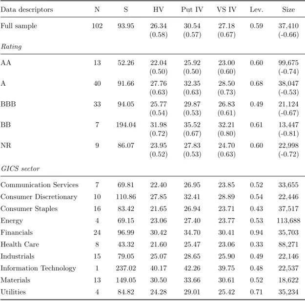
5.1 Description of data ... 46
5.2 Strategy implementation ... 48
5.2.1 Synthetic spread construction ... 48
5.2.2 Trading signals... 52
5.2.3 Hedge ratio, position mark-to-market and return aggregation 53 6 EMPIRICAL RESULTS ... 58
6.1 Model accuracy ... 58
6.2 Case study of the strategy: Anglo American plc ... 64
6.3 Strategy returns... 68
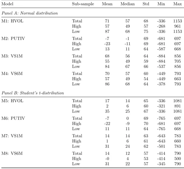
6.3.1 Holding period returns ... 68
6.3.2 Strategy monthly returns ... 74
6.3.3 Explaining strategy returns ... 80
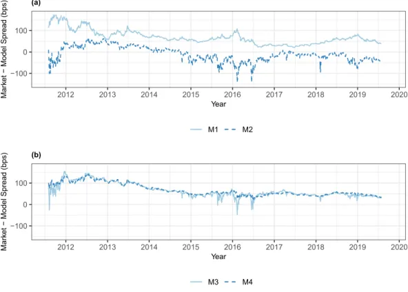
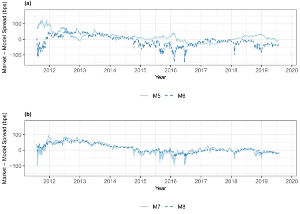
Figure 1 Mean daily estimation errors for models M1, M2, M3, and M4 . 61 Figure 2 Mean daily estimation errors for models M5, M6, M7, and M8 . 62
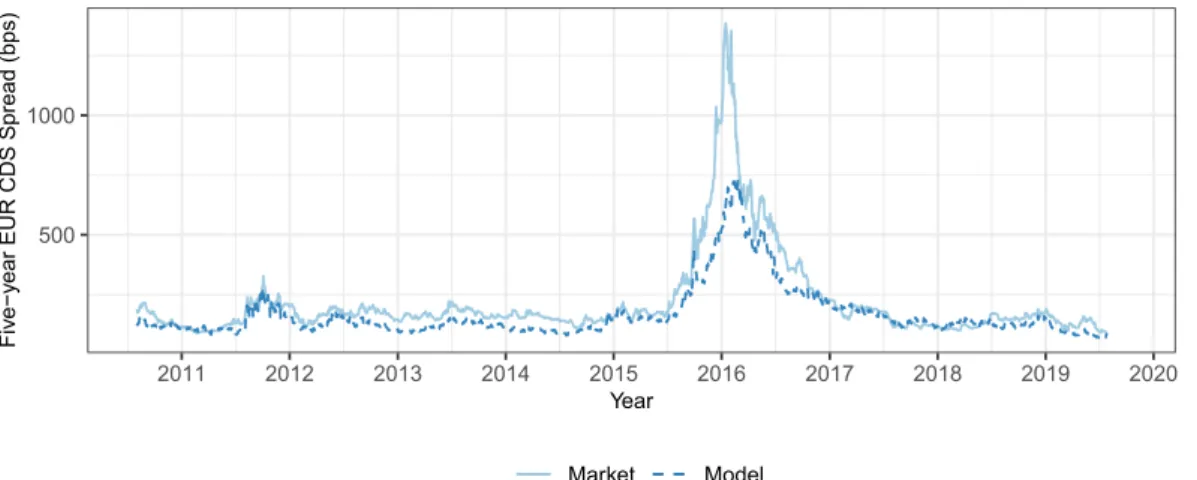
Figure 3 The five-year market CDS and M8 model spread of Anglo
American plc ... 65
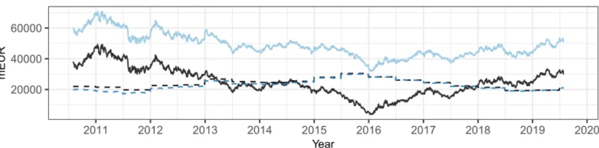
Figure 4 Model input and output for Anglo American plc ... 66
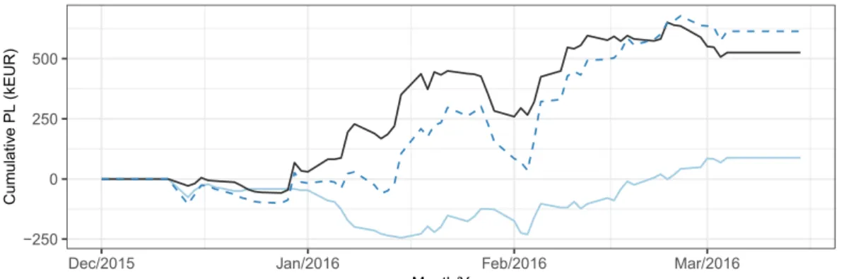
Figure 5 Trade PL breakdown ... 67
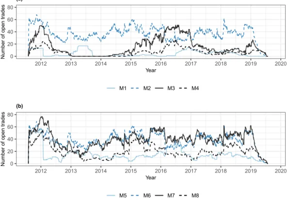
Figure 6 Number of open trades during the trading window... 72
Figure 7 Total cumulative PL of strategies with a trading trigger of 0.5 . 78 Figure 8 Net positioning of strategies with a trading trigger of 0.5 ... 79
LIST OF TABLES
Table 1 Summary table describing sample details and applied method-ologies in previous capital structure arbitrage studies... 33Table 2 Sample description and statistics ... 49
Table 3 Model estimation error statistics categorized based on calibra-tion methodology and sample credit quality ... 59
Table 4 Optimal degrees of freedom for models M5, M6, M7, and M8 ... 60
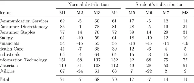
Table 5 Mean estimation errors for different model specification organ-ized based on GICS sectors... 63
Table 6 Holding period return statistics for models M1, M2, M3, and M4 ... 70
Table 7 Holding period return statistics for models M5, M6, M7, and M8 ... 71
Table 8 Monthly strategy excess return statistics for models M1, M2, M3, and M4 ... 76
M7, and M8 ... 77 Table 10 Regression results of monthly returns – Model M8 with a
trad-ing trigger of 0.5 ... 81 Table 11 Regression results of monthly returns – Model M5 with a
trad-ing trigger of 0.5 ... 91 Table 12 Regression results of monthly returns – Model M6 with a
trad-ing trigger of 0.5 ... 92 Table 13 Regression results of monthly returns – Model M7 with a
trad-ing trigger of 0.5 ... 93 Table 14 Regression results of monthly returns – Model M8 with a
trad-ing trigger of 1.0 ... 94 Table 15 Regression results of monthly returns – Model M8 with a
1
INTRODUCTION
1.1
Background
Before the financial meltdown of 2008, Boaz Weinstein – a renowned chess grand-master and the youngest-ever managing director at the global investment bank behemoth Deutsche Bank – was in charge of an internal trading group focusing on market making and proprietary trading in a variety of credit and equity in-struments. His group, called Saba, had been extremely successful during an era characterized by the wild rise of proprietary trading schemes backed by major investment banks. Weinstein and his fellow trades reportedly raked in annual profits between $600 and $900 million during the years 2006 and 2007 alone. In the preceding eight-year period, returns were also significant and consistently pos-itive. Dubbed as the world’s best credit trader, Weinstein specialized in a strategy called capital structure arbitrage in which relative value positions are formed to benefit from misalignments in the pricing of firms’ capital structures. In this study, this somewhat mysterious strategy and its profitability are analyzed by combin-ing a new post-financial crisis sample consistcombin-ing of 102 European obligors with a novel implementation methodology. Coming back to Mr. Weinstein, the year 2008 turned out to be catastrophic for him and for his team as losses of approximately $1.8 billion occurred. (Wall Street Journal 2009; Saba Capital 2020) Based on this anecdotal evidence, it seems that the strategy exhibits characteristics similar to tail risk insurance selling. This question, and many others, are addressed in this master’s thesis.
Capital structure arbitrage, sometimes called credit arbitrage or credit-equity trading, belongs to the class of fixed income arbitrage strategies where the aim is to identify and ultimately take advantage of temporary mispricings between company’s equity and debt instruments (Duarte, Longstaff & Yu 2006, 787-788; Yu 2006, 47). The development of the credit derivatives market accompanied by the belief among practitioners that cross-asset pricing misalignments can occasion-ally occur led to the wide-spread usage of this strategy among hedge funds and proprietary trading desks at the beginning of this millennium (Ju, Chen, Yeh & Yang 2015, 90; Wojtowicz 2014). Before the development of credit default swaps (CDS), market participants used bonds and equities to utilize these opportunities. Later, however, bonds were often replaced with credit default swaps due to their appealing characteristics when it comes to risk and liquidity (Ju et al. 2015, 90).
typical strategy of this kind relies heavily on a structural credit risk model that takes as inputs company’s liabilities and the market value of its equity. The output, on the other hand, is a default measure or a credit spread. The most famous structural credit risk model is the one developed by Merton (1974), which sees a firm’s equity as a European call option on its total assets. This revelation enables the use of Black & Scholes (1973) type of framework when deriving the default probability measure. To iterate the strategy implementation further, one can now utilize the Merton (1974) model default measure and calculate a synthetic CDS spread. By comparing this synthetic CDS spread to market quotes, it is possible to engage in trades that would be profitable in the case of convergence. For example, if the synthetic CDS spread is notably higher than the market quote, that would imply – assuming that the model is correct – that the equity market has a more negative view on company’s credit quality compared to the CDS market. If the equity market is assumed to be correct in its view, the rational move would be to buy protection from the CDS market. If the market spread eventually converged with the synthetic quote, the mark-to-market of the position would in this case be positive. In a situation where a market participant does not want to address which market is pricing the risk correctly, a position can be taken on both markets by using a predefined hedge ratio to correctly scale the two trades. (Yu 2006, 47) The enthusiasm that capital structure arbitrage sparked at the beginning of this millennium has encouraged academics to analyze the execution and profitab-ility of this strategy rather thoroughly (see Yu 2006, Duarte et al. 2006, Bajlum & Larsen 2008, Imbierowicz & Cserna 2008, Wojtowicz 2014, Ju et al. 2015, Huang & Luo 2016 and Zeitsch 2017). The overall results of these studies are supportive of the strategy. Still, many of these studies highlight the risks that arise from single positions that end up diverging instead of converging. In light of this evidence, it is essential to understand that this strategy is far from being a textbook example of arbitrage since the positions are based on a model that can be calibrated and adjusted in many ways. Lastly, instrument level strategy execution naturally af-fects the results regarding profitability. Earlier studies focus on trading equities relative to credit default swaps, while some of the latest research looks into equity options as a possible substitute. The rationale behind the use of equity options is to hedge the CDS leg against fluctuations in option implied equity volatility instead of hedging the effects of equity price movements. In option jargon, this would translate into hedging vega instead of delta. If only the correlations between changes in equity prices or implied volatility against CDS spreads are looked at, no large differences can be observed. However, the sensitivity between the CDS spread and option-implied equity volatility is several orders of magnitude higher
than the sensitivity between CDS spreads and equity prices. (Zeitsch 2017, 8;12) Given this information, smaller and less capital intensive positions are needed to hedge the CDS positions if instruments linked to equity volatility are used.
To take this vega hedging approach a one step further, variance swaps are analyzed in this thesis instead of equity options. Briefly, variance swaps are over-the-counter derivatives that enable the investor to take views on future realized volatility against current implied volatility (Bossu 2006, 50). Compared to options, variance swaps provide a purer exposure to future volatility or, technically, to future variance.1 Thus, variance swaps are the most fitting instrument to truly
test if the vega hedging approach should be considered as a valid alternative to its more traditional delta hedging counterpart.
1.2
Research problems
The research problems aimed to be addressed in this study can be divided into two broad categories, namely into the model and strategy-specific problems. Let us start with the model-specific ones. The structural model of choice in this thesis is the Merton (1974) model mentioned above. To ultimately calculate default probab-ilities for the synthetic CDS spread, the methodology of Moody’s KMV is applied.2
In itself, it is interesting to analyze the Moody’s KMV Merton (1974) model in a capital structure arbitrage setting since typically the CreditGrades model is selec-ted in previous studies (see, e.g., Yu 2006, Duarte et al. 2006, Bajlum & Larsen 2008 and Wojtowicz 2014).3 Furthermore, it has been well documented that the
Merton (1974) model generally produces credit spreads that are significantly lower compared to market spreads (see, e.g., Ogden 1987, Lyden & Saraniti 2001 and Eom, Helwege & Huang 2004). In order to address this issue, among others, various model calibration methodologies are analyzed in terms of mean spread estimation errors.
It can be said that the most critical consideration in the calibration process is the choice of equity volatility. In order to solve the latent model parameters such as asset volatility, an estimate of equity volatility has to be provided. Typically, average historical volatility has been used in the calibration (see, e.g., Yu 2006,
1The contract is based on variance or volatility squared instead of volatility due to valuation and
hedging reasons (Demeterfi, Derman, Kamal & Zou 1999, 3).
2Regarding Moody’s KMV, see Crosbie & Bohn (2003).
3For a detailed description of the CreditGrades model, see Finger, Finkelstein, Lardy, Pan, Ta
Imbierowicz & Cserna 2008 and Bajlum & Larsen 2008). This simple approach, however, produces spreads that are not sensitive to changing market conditions. To improve the accuracy and sensitivity of the synthetic spread, deep out-of-the-money put implied volatility alongside with variance swap rates are used in this thesis, and thus compared to results generated with historical volatility. Compared to deep out-of-the-money or at-the-money implied volatilities, variance swap rates reflect implied volatility given the whole range of strikes, thus incorporating all the information contained in the volatility surface. Overall, the relationship between CDS spreads and option-implied volatilities have been studied extensively by, for example, Carr & Wu (2009). When determining the unknown credit parameters, i.e., calibrating and eventually solving the structural model parameters, practition-ers and academics alike argue that by utilizing the equity options market instead of just the equity market, more accurate results can be achieved (Elkhodiry, Paradi & Seco 2011, 46). Moreover, in capital arbitrage studies in which implied volatility is used to calibrate the structural model, the achieved synthetic spread accuracy seems promising (see, e.g., Zeitsch 2017).
As said, volatility calibration plays a key role in terms of model accuracy and responsiveness. However, the distribution used to determine default probabilities has an essential role as well. With the Moody’s KMV model applied in this study, the simplest solution is to rely on the normal distribution, as is the case in the cap-ital structure arbitrage study conducted by Zeitsch (2017). Nevertheless, Crosbie & Bohn (2003) already note that this simple approach does not come without its drawbacks. The fact that the total asset value representing a point of default for the obligor, also known as the default barrier, is indeed random undermines the underlying assumption regarding the deterministic relationship between default probabilities and the Merton (1974) model default measures. Further, Crosbie & Bohn (2003) highlight that the empirical default distribution exhibits fatter tails and hence higher kurtosis than the normal distribution. To avoid these above mentioned pitfalls, Crosbie & Bohn (2003) utilize a proprietary empirical distri-bution to map default probabilities. In this thesis, the aforementioned challenges are combated and analyzed by taking advantage of the Student’s t-distribution, and then testing whether model accuracy and strategy returns are affected. Ad-ditionally, a fully risk-neutral calibration, i.e., a calibration which only relies on market-implied data instead of historical figures, is tested. In this approach, not only volatility calibration is risk-neutral, but also, the default barrier is derived in a risk-neutral manner. This is done by following the novel methodology introduced by Zeitsch (2017). By taking advantage of the risk-neutral default barrier, obligors
with unusual capital structures, such as financials, can be included in the sample, and thereby it is feasible to test the methodology’s effectiveness.4
Put more formally; the model-specific research questions are the following:
• Is the Merton (1974) Moody’s KMV model comparable to other applied models in terms of model accuracy and strategy profitability?
• Does the use of implied volatility and variance swap rates improve model responsiveness compared to historical volatility?
• How the use of t-distribution instead of the normal distribution affects model accuracy?
• What is the impact experienced by applying a risk-neutrally calibrated de-fault barrier? Does it improve results especially with financials?
Moving on to the other main focus of this thesis, i.e., to strategy-specific re-search problems. Consequently, strategy returns are intertwined with the tested model calibration methods because unbiased trading signals play an essential role in a successful implementation. Hence, these two focus areas should not be ana-lyzed in isolation. Considering that in most of the previous capital structure arbit-rage studies stocks are used to hedge the CDS positions, the use of equity variance as a substitute can be seen as the most exciting theme in terms of strategy exe-cution. Even though Carr & Wu (2009) highlight that there is a clear connection between CDS spreads and implied volatility, the equity volatility component has not been thoroughly introduced as a part of the trading strategy. In previous studies, only Zeitsch (2017) uses equity options as the equity leg with promising results. For two specific reasons, it is intriguing to take advantage of variance swaps in both model calibration and strategy execution. First, the prevailing vari-ance swap rate for a particular tenor is calculated by forming a well-defined options portfolio that contains puts and calls from all available strike prices. This way, all the information in the equity volatility surface at that tenor range is summar-ized by one number. By utilizing this risk-neutral option implied measure, the calibrated structural model should, in theory, better reflect the views of the equity options market as a whole when compared to at-the-money or out-of-the-money option implied volatilities. Second, with variance swaps, a profit and loss profile genuinely dependent on the difference between implied and realized variance can be achieved. The issue with delta-hedged option positions is that the volatility
4In many capital structure arbitrage studies, financials and utilities are excluded from the sample
exposure is not pure, but instead, mostly path-dependent (Allen, Einchcomb & Granger 2006).
Other strategy-specific problems revolve around implementation methods and return characteristics. In the empirical part, individual holding period returns are analyzed as well as monthly aggregate returns. With all the tested models, different strategy implementation methods are considered for testing the robustness of the results. Moreover, different trading triggers that symbolize the threshold to open a trade are tested. To evaluate if the returns are dependent on the obligor’s credit quality, a sample consisting of 102 European obligors is divided into two sub-samples. Finally, monthly strategy excess returns are regressed on common market risk factors to understand whether returns arise from exposures to the general market. Now, strategy-specific questions can be expressed as follows:
• Can a capital structure arbitrage strategy relying on vega hedging be con-sidered as an alternative to the more traditional delta hedging approach?
• How model calibration methodology affects holding period and monthly re-turn characteristics?
• Can common market risk factors explain monthly excess returns of the strategy?
1.3
Limitations of the study
Commenting on the limitations of this thesis, few mentionable themes come to the forefront. From a model perspective, only the Merton (1974) Moody’s KMV model is analyzed thoroughly in this study. As with other studies such as Imbierowicz & Cserna (2008) and Ju et al. (2015), where multiple models are tested with the same sample, this is not done here. When comparing the Merton (1974) Moody’s KMV model to other models, this is done by solely relying on the information provided by previous studies. With strategy implementation, only the vega hedge approach is tested. Corresponding to the practice with model comparisons, previous studies are used as a benchmark.
To simplify the empirical analysis, only a strategy utilizing six-month variance swaps is tested with all the model variants. Additionally, the maximum holding period is set to 180 days with all the tested strategies. This practice is in contradic-tion with previous studies where different maximum holding periods were analyzed as well. Again, this is done to simplify the analysis and to match the traded tenor
with the selected maximum holding period. On a theoretical level, a closer link between the model calibration inputs and the traded instruments should lead to improved performance. Using shorter than the six-month tenor implied volatilities and variance swap rates in the model calibration leads to a mismatch between the trading signal and traded instruments. A mismatch of this sort could ultimately undermine the strategy’s profitability.
Moreover, there are some challenges that arise from the use of variance swaps. Because the instrument only trades over the counter, the actual market quotes are somewhat invisible. However, relying on quotes constructed from prevailing option prices, an educated guess of the market price can be made. In this thesis, the variance swap data is sourced from Bloomberg. To implement the described strategy in practice, a broad network of broker-dealers should be utilized to get updated market quotes for the companies in the trading universe. As imaginable, this kind of arrangement is only attainable for large and sophisticated institutional investors.
Finally, partly due to the selected strategy implementation methodology and long trading window, the sample size is small compared to previous studies. To cover the sample starting from August of 2010 and ending in July 2019, many otherwise suitable obligors are excluded from the company universe. The second factor narrowing down the sample size is the availability of variance swap data. Nevertheless, these filters lead to a sample consisting of large European companies with both liquid CDS and options market, thus promoting the economic signific-ance of this study.
1.4
Structure of the thesis
The thesis is structured as follows. The three following chapters focus on the relevant theoretical background. More specifically, the Merton (1974) model is discussed in detail. Concepts regarding its risk-neutral calibration, default prob-ability, and hedge ratio determination are covered. Then, the focus shifts to capital structure arbitrage strategies and preceding studies from that field. Lastly on the theoretical front, credit default and variance swaps are discussed since these in-struments are used in the execution of the strategy later in this study. The fifth chapter covers data and methodology. Empirical results are then presented in chapter six, and finally, conclusions are presented thereafter.
2
MERTON MODEL AND RISK-NEUTRAL
CALIBRA-TION
2.1
Overview of the model
Credit risk can be defined as the risk that an obligor loses some or all of the funds that were borrowed to the creditor. If contractual payments cannot be made on time, this constitutes a default on the creditor’s side. A default can also occur similarly in a credit derivative contract when the counterparty is unable to deliver the payment specified in the terms of the contract. (Hull 2012, 521) If one desires to calculate the credit risk of the creditor or the counterparty, one must determine the probability of default for that entity. To calculate the probability of default (PDF), either reduced-form or structural credit risk models can be used. Reduced-form models are formulated around the assumption that credit events occur randomly, and that the main driver behind default is an exogenous factor. The randomness in these models is commonly built around a Poisson process.5
(Chatterjee et al. 2015, 13) Unlike reduced-form models, structural credit risk models consider the balance sheet of the company in question, and see the default arising from endogenous factors instead. The pioneering model in this class of credit risk models is the Merton (1974) model. (Elkhodiry et al. 2011)
The focus of this study is on the Merton (1974) model partly due to its sim-plicity, but also due to its theoretical implications given the capital structure ar-bitrage setting at hand. Here, the purpose is to utilize the model to calculate default probabilities for different entities. To emphasize, the model is not used to calculate credit spreads but rather to produce probability estimates that can be later used as an input when calculating the synthetic credit default swap spreads. Since financial derivatives such as CDS contracts and options are priced under the neutral measure, the Merton (1974) model is later calibrated so that risk-neutrality will not be violated. This is achieved by following the methodology discussed mainly by Zeitsch (2017), where the asset drift µ is assumed to equal
the risk-free rate r. Additionally, asset volatility, i.e., volatility of the asset value,
and the default barrier – an asset value level signifying a point of default – are calibrated without the use of historical or real-world probabilities. Nevertheless, a model calibrated with historical volatility is also tested to see whether the risk-neutral model calibration methodology is genuinely preferable. Next, the Merton (1974) model, its assumptions, and derivation are covered in detail. Then,
set volatility and default barrier are defined so that default probabilities can be discussed, and eventually calculated.
To get a more thorough understanding of the Merton (1974) model, let us consider a scenario where a firm consists only of a single zero-coupon bond that matures at time T, and of an equity security that is the residual claim on the firm’s
total assets V. In this specification, the firm can only default at time T. If the
company is not able to return the principal of the bond at time T, all the remaining
assets will be owned by the bondholder. In the case of default, the equity holder will receive nothing. If the firm can make the principal payment at time T, the
equity holder is entitled to the assets that remain after the payment. Additionally, it must be assumed that the company will not issue new debt that outranks the outstanding claim and will not pay dividends or engage itself in stock buybacks before time T. Now, let us additionally assume that the firm’s asset dynamics
follow geometric Brownian motion and can be written
dVt=rVt+σVVtdWt,Q, (1)
where Vt is the value of the firm’s total assets at time t, r is the risk-free rate, σV
is the asset volatility and dWtis the Wiener process under risk-neutral probability
measure Q.6 (Merton 1974, 450-453) Both r and σ
V are regarded as constants.
Suppose that the value of the zero-coupon bond B is dependent only on the value
of the firm and time. The price of the bond is now given by B = F(V, t) and the following stochastic differential equation represents the dynamics of its return process
dBt =αBBt+σBBtWt, (2)
where αB is expected return of the bond during a specified period, e.g., during a
year, Bt is the value of the bond at time t, σB is the volatility of the bond and Wt
is the standard Wiener process under real-world probability measure P. By using the Itô–Döblin theorem, Equation (2) can be written
dBt= [︄ 1 2σ 2V2F V V +αV FV +Ft ]︄ dt+σV FVdWt, (3)
where FV, FV V and Ft stand for partial derivatives with respect to V and t.
(Merton 1974, 451) To simplify notation, subscript t is omitted from the total
asset valueV. Following the replication argument7 of Merton (1973) which can be
used to prove the Black & Scholes (1973) model, and by simplifying, Equation (3)
6The dynamics of the asset value process are presented under the assumption of risk-neutrality.
can be formulated as follows 1 2σ
2V2F
V V +rV FV −rF −Fτ = 0, (4)
where τ = T −t is the time to maturity and Ft = −Fτ. (Merton 1974, 453) To
solve this equation, one must first define an initial condition and two boundary conditions. In this specification, V ≡F(V, τ) +f(V, τ), where f(V, τ)is the value of equity and thus can expressed f(V, τ) =Sτ. Since neither the value of debt or
equity can be negative, the first boundary condition takes the following form
F(0, τ) =f(0, τ) = 0. (5)
Due to the fact thatF(V, τ)≤V, the second boundary condition is (Merton 1974,
453)
F(V, τ)
V ≤1. (6)
The initial condition arises from the assumptions that were laid out earlier. If
V > F(V,0), the firm will pay back the zero-coupon bond and due to the residual claim of the equity holder, the value of equity isf(V,0) =V −F(V,0) = V −B. In
a scenario whereV < F(V,0), the debt holder would take control of all remaining assets of the firm and the equity value would simply be zero. Based on this logic, at time τ = 0 the initial condition for the value of debt is simply (Merton 1974, 453)
F(V,0) = min[V, B].
Given these conditions, it would be possible to solve the value of debt, and eventually, the unknown asset value, but instead of doing that, a more common approach can be utilized. Let us focus on the value of equity more closely. To formalize the residual claim and limited liability that the equity holder possesses, we write f(V, τ) = min[0, V −F(V, τ)]. By rewriting the Equation (4) so that
F(0, τ) =f(0, τ), the partial differential equation for equity is naturally 1
2σ
2V2f
V V +rV fV −rf −fτ = 0, (7)
and correspondingly, the initial condition is given by
f(V,0) = max[0, V −B].
To get the boundary conditions for this partial differential equation, we replace
F(0, τ) with f(0, τ) and rewrite the boundary conditions (5) and (6). (Merton 1974, 453)
ended up with an equation and boundary conditions that match the ones presented by Black & Scholes (1973).8 The European call valuation methodology in Black &
Scholes (1973) is now extended into the valuation of the firm’s total assets. The nominal debt amount B takes the place of the strike price, and asset value V is
naturally the underlying asset of the contract. Equity value f(V, τ)can be written in the following well-known form when σV is assumed to be a constant (Merton
1974, 453–454) f(V, τ) =VΦ(d1)−Be−rτΦ(d2), (8) where Φ(d) = √1 2π ∫︂ d −∞ e−12z2dz, and d1 = ln(︁VB)︁+(︁r+12σV2)︁τ σV √ τ (9) d2 =d1−σV √ τ . (10)
In order for the model to hold, certain assumptions need to be made. These include the so-called perfect market assumptions, and the possibility to trade con-tinuously, the idea proposed by Modigliani & Miller (1958) that firm’s value does not depend on its capital structure, flat term structure of interest rates, and that the asset value follows the dynamics presented in Equation (1). Most of these assumptions can be relaxed. However, assumptions regarding continuous trading and asset value process are essential. (Merton 1974, 450)
The primary critique of the model has been circulating around the low credit spreads, i.e., corporate bond prices, it produces. In the class of high yield bonds, the pricing errors are even more pronounced compared to investment-grade bonds. (Eom et al. 2004, 499) Research has focused on the relatively unrealistic assump-tions of the model, and after the publication of Merton’s (1974) seminal paper, many papers that introduce alternations to the original model have been pub-lished. Among the most notable pieces of research are Black & Cox (1976), Geske (1977), Longstaff & Schwartz (1995), Leland & Toft (1996) and Collin-Dufresne & Goldstein (2001).
Black & Cox (1976) introduce the idea that restructuring might take place before the maturity of the bond. Geske (1977), on the other hand, incorporated coupon paying bonds into the analysis. Longstaff & Schwartz (1995) use stochastic interest rates and assume a constant recovery rate9 while Leland & Toft (1996)
8Equation (7) and the boundary conditions presented here match the Equations (7) and (8) in
Black & Scholes (1973, 643).
9Recovery rate is the value of the liability given default. They are typically quoted as a fraction
create a model in which the firm issues regularly new debt with a fixed maturity. In the Leland & Toft (1996) model, the equity holders can issue new equity to cover the debt payments or simply default on their obligations. Furthermore, Collin-Dufresne & Goldstein (2001) base their model on the findings of Longstaff & Schwartz (1995) and restrict the amount of leverage by using a stationary leverage ratio. Now one might ask whether these alternative representations perform better than the original model. Eom et al. (2004) analyze the aforementioned alternative models in detail, and find that all of the models produce on average significant prediction errors compared to credit spreads of non-callable corporate bonds.
In this thesis, the model of choice is the original Merton (1974) model even though some of its assumptions are indeed relatively unrealistic. As was high-lighted by Eom et al. (2004), the spread prediction accuracy of the more soph-isticated models was weak as well. Hence, the use of some alternative structural model in this study cannot be seen to be the most relevant choice available. The aim here is not to use the Merton (1974) model in spread prediction but instead in default probability determination, and thus the focus will be on model calibration and parameter selection. Next, these aspects are discussed in detail.
2.2
Asset volatility and the default barrier
Continuing with Equation (8), it can be observed that the value of the callf(V, τ)is already known since it represents the market capitalization of the firm. Conversely, the face value of debt B, in Merton’s specification, is not as straight forward to
characterize because it can be defined in two ways when dealing with real-world applications. First, it can be seen as the firm’s total liabilities, and thus a simple balance sheet value can be used. Alternatively, though, the parameter can be said to represent an asset value level that signifies default. If the firm’s asset value drops significantly and hits this so-called default barrier, the firm is in default. To calculate an estimate for the firm value V at time t, parameter B must first be
determined. Another latent and also the most important parameter in the model is asset volatility σV which appears in Equations (9) and (10) (Zeitsch 2017, 8).
In this section, these parameters are discussed, starting with asset volatility, and then moving on to a more granular presentation of the default barrier.
In asset volatility determination, multiple different methodologies can be used. However, only the three most fundamental methods are covered here; those be-ing the proxy method, maximum likelihood method, and the volatility restriction
method (see, e.g., Li & Wong 2008). The proxy method, first introduced by Jones, Mason & Rosenfeld (1984), relies on an asset value approximation calculated from market values and book values alike. After asset value estimates have been cal-culated covering a certain period, a time series can be constructed, and then the volatility of assets calculated. The maximum likelihood methodology, initially proposed by Duan (1994), builds on the assumption that the firm value follows a log-normal distribution. Hence, asset volatility can be determined by maximizing the suggested likelihood function. Finally, the volatility-restriction method, which, according to Li & Wong (2008), is the most popular method used in structural models, is implemented by simultaneously solving two equations that originate from the Merton (1974) model. Following the methodology pioneered by Ronn & Verma (1986), the two equations are
St=CBlack–Scholes[Vt, σV, τ, Bt, r] (11) and σS = (︄ Vt St )︄ ∂St ∂Vt σV (12)
where S is the equity market capitalization. Equation (11) corresponds with the
definition of equity value given by the Merton (1974) model, and Equation (12), on the other hand, can be derived by applying the Itô–Döblin theorem and following the assumption that the value of the firm’s equity is dependent only on the firm value V and time to maturity τ. Now, asset volatility and ultimately the asset
value can be solved by first estimating equity volatility σS and then finding a
solution that satisfies these equations. This iterative procedure is repeated at each time point when asset volatility and asset value must be calculated. Given the popularity of the volatility restriction method, it is crucial to understand its challenges. Firstly, it violates the assumption of constant volatility in the Merton (1974) model (Li & Wong 2008, 754). Additionally, as Duan (1994) notes, the major issue with this methodology is the underlying proposition that Itô–Döblin theorem and related assumptions must hold at every time point. This proposition, however, is hardly true since equity prices might exhibit sudden and relatively large jumps.
In this thesis, a somewhat similar methodology introduced by Zeitsch (2017) is followed. Starting with Equation (12) as an initial representation, let us define essential boundary conditions for the asset value Vtat timet. Firstly, the following
must hold
Vt|St=0 =B ′
where B′(t, T) denotes the default barrier, which depends on current time t and
certain maturityT. To express Equation (13) more intuitively, one can think that
if the market capitalization of the firm at time t is zero, then all that is left is
the value indicated by the default barrier. Further, Equation (13) represents the behavior of firm value near default.
The second boundary condition reflects the dynamics of Vt when the firm’s
capital consists mostly of equity. Put mathematically, if S is significantly larger
than B′(t, T) and assuming that lim
B′(t,T)→0
St
Vt
= 1,
and by extending this so that
lim
B′(t,T)→0
∂St
∂Vt
= 1
we have the second boundary condition. In the expressions above, lim denotes limit. By taking the first-order approximation of Equation (13) atB′(t, T), we get
Vt≈B′(t, T) +
∂Vt
∂St
St.
As noted by Zeitsch (2017), a simple representation that respects these boundary conditions is given by
Vt≈B′(t, T) +St. (14)
Now, by combining Equation (12) with the representation in Equation (14), asset volatility σV takes the following form
σV =σS
St
St+B′(t, T)
. (15)
This expression is used to calculate asset volatility later in this study. The formula derived by Zeitsch (2017) is equivalent to the one by Finger et al. (2002), which is used as a part of the CreditGrades methodology.10 To eventually calculate the
asset volatility, estimates for the default barrier B′(t, T) and equity volatility σS
must be given.
Now, let us focus on the equity volatility parameter a little more thoroughly. In the original Merton (1974) paper, the use of historical equity volatility is suggested for the calibration. Similarly, in the CreditGrades methodology, equity volatility is calibrated with historical volatility based on an estimation window of 1000 days
10CreditGrades is a quantitative credit assessment model developed together with Deutsche Bank,
Goldman Sachs, JPMorgan, and RiskMetrics Group. It can be seen as a contender for the Moody’s KMV methodology.
(Finger et al. 2002, 19). As noted by Zeitsch (2017), the use of historical equity volatility dampens the model’s responsiveness to recent equity volatility and hence leads to an underestimation of the CDS spread. Since the goal of this thesis is to construct a model that swiftly identifies trading opportunities, the role of model responsiveness cannot be undermined.
To address this issue, implied volatility from equity options can be utilized. Given the aim to risk-neutrally calibrate the Merton (1974) model, the use of option-implied volatility is essential since it can be seen as a risk-neutral value which importantly incorporates the volatility risk premium as well (see Figlewski 2016 and Carr & Wu 2008). Moreover, it is well established in prior literature that if information from equity options is used when estimating credit-related information, results undergo a significant improvement (Elkhodiry et al. 2011, 69). For example, Bharath & Shumway (2008) find that the use of option-implied volatility instead of historical equity volatility substantially improves the out-of-sample default forecasting accuracy of the Merton (1974) model. Furthermore, studies have shown that there exists a clear link between credit spreads and option-implied volatility (see, e.g., Carr & Wu 2009 and Elkhodiry et al. 2011). This link translates into reliable results when implied volatility is used to estimate CDS spreads (Cao, Yu & Zhong 2010 and Cao, Yu & Zhong 2011). Due to this strong empirical backing, option implied volatility is primarily used to calibrate the equity volatility σS parameter later in this thesis.
Moving on to the derivation of the default barrier, it can be seen that the default barrier plays a role in the asset volatility calculations. However, the importance of this parameter is not comparable to the one of asset volatility (Afik, Arad & Galil 2012, 4). In many of the previous studies, the default barrier is assumed to be a constant that consists of short term and half of the company’s long term debt (see, e.g., Crosbie & Bohn 2003 and Vassalou & Xing 2004).11 Random default barrier
methodologies have also been used in order to generate spreads that could closely match the market spreads (see, e.g., Finger et al. 2002). For example, Elkhodiry et al. (2011) find supportive evidence towards using a random default barrier in credit spread determination. Here, the novel approach of Zeitsch (2017) is followed. This default barrier model can be said to belong to the group of random default barrier models.
Starting with Equation (13), and assuming that it holds when S approaches
11For more about the constant default barrier, see Longstaff & Schwartz (1995) and Leland &
zero we get
lim
St→0Vt =B
′ (t, T).
The aim is to find an asset value level that signifies a point of default given the asset value dynamics defined in Equation (1), a predefined maturity T, total liabilities Bt, risk-free rate r and asset volatility σV. Once again, it is possible to use Black
& Scholes (1973) methodology to solve this problem.
The first step in this iterative procedure is to set an initial value for the default barrier B′(t, T). Assuming that loss given default (LGD) is 60% of total assets, one could use the following estimate
B1′(t, T) = Bt×0.6,
where the subscript 1 represents the iteration step. Next, this estimate must be used to calculate asset volatility σV with Equation (15). Then, by continuing this
iteration procedure, a solution for B′(t, T) must be found that satisfies lim
B′(t,T)→0CBlack–Scholes[B
′
i(t, T), σV, τ, Bt]≈0, (16)
whereCBlack–Scholesrefers to the formula of a long European call by Black & Scholes
(1973), and in this instance is defined by
f(Bi′, τ) =Bi′(t, T)Φ(d1)−Bte−rτΦ(d2), whereτ =T −t and Φ(d) = √1 2π ∫︂ d −∞ e−12z 2 dz, and d1 = ln(︁Bi′ Bt )︁ +(︁ r+ 12σ2 V )︁ τ σV √ τ d2 =d1−σV √ τ .
Moreover, iin the subscript denotes iterative step i.
This novel methodology, introduced by Zeitsch (2017), allows us to define the risk-neutral default barrier. By defining the default barrier in this manner, it is allowed more accurately to reflect changing market dynamics and thus change daily. Market responsiveness is further amplified by the use of implied volatility measures when the asset volatility is calibrated. It is important note however, that because the Black & Scholes (1973) formula is a set of non-linear non-negative equations, the root of Equation (16) must be approximated. This is accomplished by utilizing the Broyden method and assuming an over 99% drop in the market
capitalization of the firm. For more about the Broyden method, see Dennis Jr & Schnabel (1996).
2.3
Default probabilities in the Merton model
To price credit default swap contracts (CDS), one has to provide probabilities of default for different maturities so that the CDS spread at time t can be
calcu-lated. In this section, the default probability calculation methodology based on Moody’s KMV methodology is covered (see, Crosbie & Bohn 2003). As said, the methodology relies on the Merton (1974) model and was initially developed by the KMV company founded by Stephen Kealhofer, John McQuown, and Oldřich Vašíček. In 2002, the company was acquired by Moody’s, hence the name Moody’s KMV. (Moody’s 2019) The parameters derived earlier are linked to the presenta-tion shown here. Addipresenta-tionally, relevant studies regarding the model’s robustness and forecasting capabilities are discussed.
Starting with the definition of probability of default, we can write
pt=P[Vt ≤B′(t, T)|Vt=0 =Vt] =P[lnVt≤lnB′(t, T)|Vt=0 =Vt], (17)
whereptdenotes the probability of default by timet,Vtfollows dynamics presented
in Equation (1) and is given by Equation (14) and B′(t, T), on the other hand, is defined in Equation (16). (Crosbie & Bohn 2003, 17; Zeitsch 2017, 5) Given the dynamics in Equation (1), the value of assets at time t is
lnVt = lnVt=0+ (︄ r− σ 2 V 2 )︄ t+σV √ tϵ,
where r is the risk-free rate, σV is the asset volatility in Equation (15), and ϵ ∼
N(0,1). Taking lnVt and substituting it in Equation (17) yields
pt=P [︄ lnVt+ (︄ r− σ 2 V 2 )︄ t+σV √ tϵ≤lnB′(t, T) ]︄ . By rearranging we get pt=P [︄ − ln Vt B′(t,T) + (︂ r−σ2V 2 )︂ t σV √ t ≥ϵ ]︄ .
Since ϵ∼N(0,1), we can see that pt =N [︄ − ln Vt B′(t,T) + (︂ r−σ2V 2 )︂ t σV √ t ]︄ , (18)
whereN denotes the cumulative normal distribution. (Crosbie & Bohn 2003, 17–
18; Zeitsch 2017, 5) From this expression, the so called distance-to-default (DD) is given by DD= ln Vt B′(t,T) + (︂ r−σ2V 2 )︂ t σV √ t ,
which is the number of standard deviations that asset value must decrease before hitting the default barrier.
Looking back at Equation (18), it is important to address the implicit as-sumption about the existence of a deterministic relationship between the default probability and the DD measure (Campbell, Hilscher & Szilagyi 2008, 2914). Em-pirically, however, this does not seem to hold because the point of default in terms of asset value is in itself random. To handle this somewhat unrealistic assumption, a specific distance to default value is mapped to a default probability based on historical data in the original Moody’s KMV model. (Crosbie & Bohn 2003, 18) Moreover, as noted by Crosbie & Bohn (2003), when the empirical distribution is compared to the normal distribution, the tails of the empirical distribution are significantly fatter.
When analyzing the performance of the Merton (1974) DD model, one can either evaluate the default ranking or default probability estimation performance of the model. When Merton (1974) model is used to rank firm by their default risk, the results are promising. With default probability estimations, the perform-ance has been slightly poorer. (Jessen & Lando, 2015, 493) In Vassalou & Xing (2004), they analyze how default risk affects equity returns by using the Merton (1974) model to calculate a default likelihood indicator (DLI) for individual firms in their sample. They follow Moody’s KMV methodology with the exception of utilizing the normal distribution and find that the calculated DLI captures inform-ation regarding future defaults when the effects of firm size and asset volatility are controlled. Similarly, Bharath & Shumway (2008) find that the distance to de-fault measure in the Moody’s KMV methodology can be utilized when forecasting defaults. However, according to their study, this is mostly due to the functional form of the distance-to-default measure. Moreover, they conclude that default probabilities calculated with the Merton (1974) model cannot be accepted to be a sufficient statistic for the probability of default.
In light of this evidence, Merton (1974) model seems not to be the most optimal method when calculating default probabilities if one has to rely on the normal dis-tribution. To still benefit from the functional form of the model while averting these challenges, Student’s t-distribution is tested alongside the normal distri-bution in this study. To to further improve the responsiveness of the synthetic model spread, these distributions are implemented together with the risk-neutral calibration methodologies discussed earlier. By testing both the normal and the t-distribution, it is conceivable to analyze the effects arising from distribution se-lection precisely.
3
CAPITAL STRUCTURE ARBITRAGE
3.1
Strategy description
Capital structure arbitrage, a rather prominent strategy among hedge funds be-fore the financial crisis, can be described as a relative value trading strategy that involves an equity and a debt instrument of a specific firm (Duarte et al. 2006, 787– 788). To successfully find these relative value trading opportunities, it is essential to use a model that links the firm’s equity and debt instruments pricing-wise. The link can be established by taking advantage of a structural credit risk model, such as the Merton (1974) model. (Yu 2006, 47) The selected model is used to identify whether the pricing of these two instruments is consistent. If large misalignments can be found, the arbitrageur will construct a position that includes the equity and debt instruments of a specific firm. The weights and exact positioning depends on the hedge ratio and on the signal given by the structural model. For example, if the pricing of the debt instrument given the price indicated by the model seems to be too low, the trader will establish a long debt position and a complementary short equity position. The trader benefits if the price of the debt instrument even-tually rises and thus converges with the model price. If the misalignment between the model and market price is regarded to be fundamental, the equity price should not move markedly during the trade. Moreover, on a trade level the strategy is based on an idea of utilizing a temporary mispricing between firm’s equity and debt instruments.
Since the development of the global CDS market, the main debt instruments used in capital structure arbitrage strategies have been credit default swaps instead of corporate bonds. Higher liquidity and purer credit risk reflection of credit default swaps have been among the main contributors behind this trend. (Ju et al. 2015, 90) The equity leg has been typically constructed by simply trading the stocks of the company in question. However, the strong linkage between firm’s CDS and implied equity volatility as documented by, e.g., Carr & Wu (2009) has motivated the use of equity options as well.12 To give a specific example of
the implementation with these instruments, one must first understand the role of the structural model used. To judge whether an "arbitrage" opportunity exists, the structural model is applied in the default probability determination process. Next, this probability is used to calculate a synthetic CDS spread that serves as the strategy’s trading signal. To demonstrate the typical strategy implementation
used in, e.g., Yu (2006), let us denote the synthetic model spread at time t as CDSmodel,t and the market CDS spread as CDSmarket,t. Additionally, let us callα
as the trading trigger, which is expressed in percentage terms. Now, a long CDS position is opened if
CDSmodel,t>(1 +α)×CDSmarket,t,
and hedged with a long equity position, which is sized based on the calculated hedge ratio. If options are traded instead of equities, a short volatility position should be opened. For example, this translates into selling put options. If, on the other hand,
CDSmarket,t>(1 +α)×CDSmodel,t,
a short CDS position combined with a short equity position is opened. In options terms, a long volatility position should be opened by, for example, buying put options. Typically, the trading trigger α is either 50%, 100% or 200% while the
maximum holding period for a single trade varies between 30 days to 180 days (see, e.g., Yu 2006, Duarte et al. 2006 or Ju et al. 2015) A position is closed if it the model spread converges with the market spread, i.e. CDSmodel,t ≈ CDSmarket,t,
the maximum holding period is reached or a preset maximum drawdown limit is crossed. The position is profitable if the CDS position converges while the equity market acts as indicated by the hedge ratio. However, as is evident in the literature, individual positions might be extremely risky due to further divergence of both the CDS and equity positions. If the maximum drawdown or holding period limit is hit often, the strategy’s aggregate performance might suffer significantly.
As can be seen, the model used to generate the trading signals, i.e., calcu-late the synthetic CDS spread, plays a central role in the strategy execution. In the academic literature, the CreditGrades model13 and the previously discussed
Merton-based Moody’s KMV model14 are the most used ones. The CreditGrades
model, initially developed by a consortium of investment banks and research firms to standardize and improve credit risk management methodologies, is a structural model with a different functional form than the Moody’s KMV model (Finger et al. 2002, 1;9). Additionally, there are some differences regarding parameter estima-tion in the original representaestima-tions of the models. To focus more on the parameter estimation, one should set sights on the most important input parameter in a structural model: volatility (Zeitsch 2017, 8). Since the aim is to benefit from misalignments in markets that should price new information relatively effectively,
13Finger et al. (2002).
responsiveness is a central model characteristic.15 Search for responsiveness and
the encouraging results of many academic studies (see, e.g., Cao et al. 2010 and Cao et al. 2011) have motivated the use of implied equity volatility instead of historical volatility when calibrating the model. Responsiveness can be likewise improved by applying a random default barrier methodology (see, e.g., Finger et al. 2002). Next, studies regarding capital structure arbitrage are discussed in detail. Additionally, time is spent to discuss why it seems to be possible to earn excess returns by following the strategy.
3.2
Empirical evidence: Results, implementation and
mar-ket efficiency
After the turn of the millennium, capital structure arbitrage started to catch the practitioners’ and academics’ attention. As one of the first extensive studies in the field, Yu (2006) analyses the returns and risks associated with a capital structure arbitrage strategy by using credit default swaps and equities in the implementation. A sample ranging from the year 2001 to 2004 consisting of 261 North American firms is analyzed. Using a CreditGrades model calibrated with 1000-day historical equity volatility, Yu (2006) finds that with a maximum position holding period of 180 days, the strategy offers positive mean holding period returns from 0.13% to 1.01% depending on obligor’s credit quality and the strategy setup. Applying a trading trigger of 50%, the mean aggregate monthly return for obligors with speculative credit ratings is 2.78%. To consider transaction costs, Yu (2006) uses a 5% bid-ask spread for CDS trades. The costs of equity trades are neglected. However, the profitability of the strategy is highly dependent on the strategy setup. In the implementation, a position is closed if the model spread converges with the market spread. Given a 30-day maximum holding period, almost none of the trades converged, resulting in a situation where the mean holding period return is negative or marginally positive. Due to the model’s weak responsiveness and low correlation between CDS spreads and equities, the losses on individual positions are occasionally significant, Yu (2006) concludes.
Using the same sample period and size as Yu (2006), Duarte et al. (2006) utilize the CreditGrades model calibrated with 1000-day historical volatility and find that the strategy on an aggregate level leads to positive mean returns and high Sharpe ratios thus matching the findings of Yu (2006). They find that the
strategy returns have positive skewness; hence the strategy cannot be identified to rely on selling tail risk insurance.16 Moreover, four out of the six strategies tested
in the study show positive alphas at a 10% significance level when regressed with Fama & French (1993) three-factor model and other asset class excess returns. Regardless of the positive alphas, Duarte et al. (2006) report that the strategy is somewhat driven by market risk and is likewise cyclical.
Following Yu (2006) and partly Duarte et al. (2006), Bajlum & Larsen (2008) aim to solve the issues regarding responsiveness of the structural model when calibrated with historical volatility. Since the fundamental idea behind the strategy is to find a mispricing between company’s equity and debt instruments, one can see that a calibration methodology that helps to find trading opportunities more swiftly is preferable compared to a methodology that leads to unresponsive model output. To test this, Bajlum & Larsen (2008) calibrate the CreditGrades model with implied equity volatility and historical volatility. Following Yu (2006) with the strategy implementation by using a maximum holding period of 180 days and a trading trigger of 200%, Bajlum & Larsen (2008) find that for speculative-grade obligors the mean holding period return is 2.64% if the calibration is done with historical volatility. By using implied equity volatility in the calibration, a mean holding period return of 4.61% is achieved for these obligors. For investment-grade obligors, the difference in returns is less significant. Furthermore, Bajlum & Larsen (2008) report that the use of implied volatility resulted in a higher rate of convergence, thus addressing the issues with model unresponsiveness.
Continuing with studies aiming to improve model accuracy and responsiveness, Ju et al. (2015) use the multi-period Geske & Johnson (1984) model modified by Chen & Yeh (2006) (from now on the extended Geske & Johnson (1984) model) to test whether the model performs better than the CreditGrades methodology in a capital structure arbitrage setting. With the Geske & Johnson (1984) model, it is possible to consider a debt structure that consists of obligations with different maturity dates, whereas the CreditGrades model sees liabilities only as one ob-ligation with a single maturity date (Ju et al. 2015, 99). They use a sample of 369 North American obligors starting from 2005 and ending in 2008 and follow Yu (2006) with the strategy implementation. By calibrating the model with 1000-day historical volatility and using similar transaction cost methodology as Yu (2006), Ju et al. (2015) report monthly median returns ranging from 0.61% to 4.28% with the extended Geske & Johnson (1984) model and median returns from 0.57% to
16A strategy that most of the time offers steady positive returns with low volatility but might
3.97% with the CreditGrades model.17 Hence, according to the results above and
based on the observation that the extended Geske & Johnson (1984) model pro-duces lower pricing errors, the authors see the extended Geske & Johnson (1984) as a more preferable model compared to the vanilla CreditGrades model. Other results regarding the profitability of capital structure arbitrage strategy in their sample are somewhat contradictory to the academic consensus. For example, they find that the mean holding period returns for companies with high credit quality are higher than for companies with speculative-grade ratings. In fact, the mean holding period returns for companies with high yield ratings are clearly negative at -5.60%. Additionally, they report that the strategy returns are negatively skewed, and large losses occur, especially during the financial crisis.
With the goal of improving the implementation of the CreditGrades model and demonstrating positive excess returns offered by capital structure arbitrage, Huang & Luo (2016) calibrate the CreditGrades model with implied volatility and analyze a sample of over 200 obligors from January 2001 to June 2004. General results are in line with previous research. First of all, Huang & Luo (2016) are able to replic-ate the results of Bajlum & Larsen (2008) regarding volatility calibration. More precisely, they conclude that a model calibrated with implied volatility outper-forms the model employed by, e.g., Yu (2006), which is calibrated with historical volatility. Second, they find that the strategy returns cannot be explained by com-mon factors such as the Fama & French (1993) factors or the momentum factor. Furthermore, the results of regressions made against the excess returns of the S&P 500 Industry Index, Lehman Brothers Baa Intermediate Index or Tremont Fixed Income Arbitrage Index do not support the notion that the returns are driven by systematic factors. These results are somewhat similar than the ones of Yu (2006) and Duarte et al. (2006). Thirdly, Huang & Luo (2016) observe that the strategy returns are positively skewed thus complementing the results of, once again, Yu (2006) and Duarte et al. (2006), and also the results of Bajlum & Larsen (2008).
As one of the most recent studies discussing the strategy, its implementation and overall results, Zeitsch (2017) tests a new calibration and modeling meth-odology focusing mainly on improving the responsiveness of the model spread by using a risk-neutral calibration, i.e., employing implied market information instead of historical data. Since the methodologies and ideas presented in Zeitsch (2017) are essential from the perspective of this thesis, the paper is analyzed thoroughly. Two distinct themes separate the study conducted by Zeitsch (2017) from previous research. First, the model of choice is not the most often used CreditGrades model
but the original Merton (1974) model combined with the Moody’s KMV model. Second, the equity leg of the strategy is not executed with equities but instead with options. With this approach, the role of equity volatility as a suitable and more stable hedge for the opposite CDS trade is highlighted.
When implementing the Merton (1974) model, Zeitsch (2017) uses deep out-of-the-money (OTM) put implied volatility in the calibration process. In contrast, previous studies have focused on using at-the-money implied volatility at best.18
As is identified in the paper, volatility can be seen as the most important in-put parameter in a structural model. Model’s ability to reflect sudden changes in market sentiment and improved signal detection can be mentioned as the main rationales supporting the use of implied volatility. To further improve the respons-iveness, deep OTM puts can be utilized. Following the argumentation of Zeitsch (2017), a long CDS position can be viewed as a long put option on the firm’s total asset value. To specify, asset value can be thought of as the price of the underly-ing and value of debt as the strike price. If the market capitalization of the firm declines, ceteris paribus, the value of the long put increases, i.e., the CDS spread increases. If market participants expect the market capitalization to decline sig-nificantly, the demand for deep OTM equity puts will result in a rise of implied volatilities for these options. Hence, according to this logic, the volatilities of these deep OTM equity options can be seen to contain relevant information about the changing capital structure dynamics from the perspective of structural modeling. On top of the typical asset volatility calibration, Zeitsch (2017) takes advantage of deep OTM implied volatilities in the default barrier derivation. The aim here is to respect risk-neutrality as outlined earlier. The novel derivation allows the default barrier to reflect changes in market sentiment dynamically. Moreover, the barrier is no longer backward-looking like the default barrier parameters employed in the CreditGrades framework.
The execution of the capital arbitrage strategy of Zeitsch (2017) differs sig-nificantly from previous studies. As has been the standard in the field, stocks have been used as the equity leg in the execution. Zeitsch (2017), however, argues that this is not necessarily the optimal way. He analyses the correlations between CDS spreads, market capitalization and implied volatility, and finds that the cor-relation with the CDS spread is almost identical for both variables. Additionally, anecdotal evidence points to the conclusion that the relationship between the CDS spread and implied volatility is more linear than the one with market capitaliz-ation. Moreover, the volatility sensitivity of the market capitalization favors the
use of volatility instead of equities. To hedge, for example, a ten basis point move in the CDS spread with equities, a large position would be needed due to low sensitivity. Since a change in the CDS spread results in a relatively large move in implied volatility, a position size for the hedge is more manageable than in the aforementioned case. In the implementation, Zeitsch (2017) uses liquid options to construct the hedges. The hedge ratio is calculated empirically by first regressing the CDS spread against deep OTM implied volatility, and then by determining the option position size so that the profit and loss sensitivity of the option matches with the CDS position. To identify trading signals, Zeitsch (2017) relies not on the commonly used trading trigger approach but instead on a Euclidean distance (L2
distance) to determine the historical difference between the model and the market spread. If the distance during the last month increased significantly compared to the historical L2 distance, it strengthened. Ultimately, L2 distances are sorted
from smallest to largest and then sorted again by signal strength starting from the strongest. The top 10 signals lead to trades with equal weights. As can be seen, the strategy is very selective.
Based on a large sample starting from 2004 to 2011 and consisting of 830 companies, Zeitsch (2017) backtests the strategy outlined here. The first two years of the sample are used to calibrate the model, i.e., to calculate hedge ratios and trading signals. Then, an out-of-sample study is conducted with real market bid-ask prices. Using a maximum holding period of 6 months, Zeitsch (2017) finds that 70% of the trades are profitable with a high convergence rate of 80% and a mean holding period of 30 days. The approximately same number of short and long trades supports the claim regarding market neutrality of the strategy. Furthermore, the highest returns occur during the volatile periods of 2008 and 2009, contradicting the results of Ju et al. (2015). The most striking result with the implementation is that only 12% of the universe is traded. The total amount of trades is only 284, which is extremely low given the sample size. Perhaps the selectivity of the approach is one key factor behind the high rate of positive returns. Overall, the model spreads are, in most cases, close to the market spread resulting in the small number of trades. In light of this evidence, the approach of Zeitsch (2017) requires more analysis. In this thesis, selected parts of the methodology are tested and analyzed further with new, post-financial crisis data.
Now