Variability of structurally constrained and unconstrained functional connectivity in schizophrenia

warwick.ac.uk/lib-publications

A Thesis Submitted for the Degree of PhD at the University of Warwick

Permanent WRAP URL:

http://wrap.warwick.ac.uk/110754

Copyright and reuse:

This thesis is made available online and is protected by original copyright.

Please scroll down to view the document itself.

Please refer to the repository record for this item for information to help you to cite it.

Our policy information is available from the repository home page.

M A E G NS I T A T MOLEM U N IV ER SITAS WARWICEN SIS

Variability of Structurally Constrained and

Unconstrained Functional Connectivity in

Schizophrenia

by

Ye Yao

Thesis

Submitted to the University of Warwick

for the degree of

Doctor of Philosophy

Computer Science

Contents

1.1 MRI, functional MRI and Diffusion MRI . . . 1

1.1.1 Magnetic resonance imaging . . . 1

1.1.2 Functional Magnetic resonance imaging . . . 3

1.1.3 Diffusion MRI . . . 4

1.2 Schizophrenia Brief Introduction . . . 5

1.3 Schizophrenia Effects on Brain . . . 6

1.4 Functional Connectivity Entropy (FCE) . . . 7

1.4.1 Functional Connectivity Entropy Origin . . . 7

1.4.2 Functional Connectivity Entropy in Schizophrenia . . . 10

1.5 Hypothesis . . . 11

Chapter 2 Research Methodology 12 2.1 Participants . . . 12

2.1.1 Excluded subjects . . . 13

2.2 MRI Acquisition . . . 14

2.3 DTI processing . . . 14

2.4 fMRI processing . . . 17

2.4.1 Brain functional networks . . . 18

2.5 Entropy Calculation . . . 18

2.5.1 Functional Connectivity Entropy Meanings . . . 18

2.5.2 Functional Connectivity Entropy Calculation Method . . . . 19

2.6 Statistical inference . . . 20

2.7 Computational Model . . . 20

2.7.1 Computational model of brain networks . . . 20

2.7.2 Computational model in Schizophrenia . . . 25

2.8 Methods for Functional Connectivity Entropy Origin: Ageing Prob-lem (Section 3.1) . . . 29

2.8.1 Subjects . . . 29

2.8.2 Data Acquisition . . . 32

2.8.3 Data Preprocessing . . . 33

2.8.4 Statistical inference . . . 35

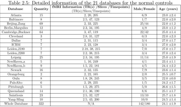
2.9 Methods for Functional Connectivity Entropy Results in Schizophre-nia (Section 3.2) . . . 35

2.9.1 Subjects . . . 35

2.9.2 Data Acquisition . . . 37

2.9.3 Data Preprocessing . . . 38

2.9.4 Statistical inference . . . 39

2.10 Functional Connectivity Entropy Properties . . . 39

2.10.1 Entropy will grow higher with more intervals in [−1,1] . . . . 39

2.10.2 Entropy vs choice of atlas: Atlases with different numbers of brain regions . . . 40

2.10.3 Entropy vs choice of atlas: Different atlases with a fixed num-ber of brain regions . . . 40

2.10.4 A mathematical description of Functional Connectivity Entropy 41 2.11 Mean, entropy and global signal . . . 44

Chapter 3 Results 47 3.1 Functional Connectivity Entropy Origin: Ageing Problem . . . 47

3.2 Functional Connectivity Entropy Results in Schizophrenia . . . 47

3.2.1 Frequency distribution of functional connectivities . . . 49

3.2.2 Functional connectivity entropy . . . 49

3.2.3 Correlation of the functional connectivity entropy with the clinical symptoms . . . 50

3.2.4 Strength of functional connectivity . . . 51

3.2.5 Summary . . . 54

3.3 Computational Model . . . 54

3.4 Structural paths . . . 55

3.4.1 Distribution of the structural paths . . . 58

3.4.2 Anatomical Distribution of Structural Paths . . . 59

3.5 Changes in Functional Connectivity Entropy . . . 60

3.6 Functional Connectivity Entropy Versus Patient Severity Score . . . 60

Chapter 4 Discussion 64 4.1 Results Summary . . . 64

4.2 Functional Connectivity Entropy in Schizophrenia . . . 65

4.3 Inspirations from Different Structural Path Results . . . 68

4.4 Limitations . . . 70

4.5 Resting fMRI Preprocessing Discussion . . . 70

4.5.1 Global Signal Correction . . . 70

4.5.2 Head Movement Correction . . . 71

4.5.3 Streamline Threshold Effects . . . 72

4.6 Functional Connectivity Entropy in Cognitive Training (Further Ap-plications) . . . 74 4.6.1 Summary . . . 74 4.6.2 Introduction . . . 75 4.6.3 Methods . . . 76 4.6.4 Results . . . 79 4.6.5 Discussion . . . 80 Chapter 5 Conclusions 84 Appendix A Appendix Figures 86 Appendix B Appendix Code 90 B.1 Matlab Code of Functional Connectivity Entropy . . . 90

List of Tables

2.1 Clinical and demographic features . . . 13 2.2 Names and abbreviations of AAL brain regions . . . 15 2.3 Neural and synaptic parameters . . . 22 2.4 Detailed information of 22 databases from the FCON 1000 Project

This table is modified from Yao et al. [2014]. . . 31 2.5 Detailed information of the 21 databases for the normal controls . . 36 2.6 Detailed information for the patients . . . 37

3.1 Distribution of the primary, secondary and tertiary paths across the 6 Resting State Networks . . . 63

List of Figures

1.1 Nuclear spins of hydrogen atoms . . . 2

1.2 Different types of MRI imaging modes . . . 2

1.3 Blood-oxygen-level dependent (BOLD) demonstration . . . 4

1.4 Diffusion MRI (Diffusion Tensor Imaging) tractography demonstration 5 1.5 The Origin of the Functional Connectivity Entropy . . . 9

2.1 Three types of structural paths defined using diffusion tractography 16 2.2 Illustration of the Functional Connectivity Entropy of the Brain . . 19

2.3 Schematic representation of the brain network . . . 23

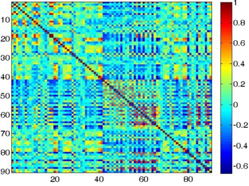
2.4 Neuroanatomical connectivity matrix . . . 24

2.5 Simulated BOLD signals . . . 26

2.6 Simulated functional connectivity matrix . . . 27

2.7 The distribution of correlation coefficients . . . 28

2.8 Excitatory neuron number versus intra-excitatory connection strength ω1 . . . 29

2.9 Average firing rate versus percent reduction of NMDA strength from the excitatory to inhibitory (E-to-I) population . . . 30

2.10 Entropy versus the number of brain regions . . . 41

2.11 10 different atlases were chosen to separate the AAL atlas into more parts . . . 42

2.12 Correlation coefficient distributions in patients and controls with global signals removed (WGR) and without global signals removed (NGR) 46 3.1 Functional connectivity entropy vs Age . . . 48

3.2 Distribution of the functional connectivity correlation coefficients . . 49

3.3 Functional connectivity entropy (FCE) for patients with schizophre-nia and controls . . . 50

3.4 Functional connectivity entropy correlated with the severity of differ-ent symptoms in the schizophrenia group . . . 51

3.5 Functional connectivity matrix . . . 53

3.6 Computational Model Demonstration . . . 56

3.7 Computational Model in Schizophrenia . . . 57

3.8 Distribution of the structural paths in patients and controls This figure is reproduced from Yao et al. [2015]. . . 58

3.9 Anatomical Distribution of Direct and Indirect structural paths . . . 59

3.10 Functional connectivity entropy in different fiber pathway . . . 61

3.11 Functional Connectivity Entropy VS SSPI score . . . 62

4.1 Effect of global signal on Functional Connectivity Entropy . . . 72

4.2 Results of using streamline threshold=2 This figure is reproduced from Yao et al. [2015]. . . 73

4.3 Results of using streamline threshold=3 This figure is reproduced from Yao et al. [2015]. . . 74

4.4 Flowchart in the trials . . . 77

4.5 Entropy change rate in cognitive training groups . . . 81

4.6 Functional Connectivity Change in training groups . . . 82

A.1 Enlarged Version of Figure 3.9 . . . 87

A.2 Enlarged Version of Figure 3.5 . . . 88

Acknowledgments

I am heartily thankful to my supervisor, Jianfeng Feng, whose encouragement, guid-ance and support from the initial to the final level enabled me to develop an under-standing of the subject.

Secondly, I offer my regards and blessings to all of those who supported me including Prof. Edmund Rolls, Prof. David Waxman, Prof. Lena Palaniyappan and Prof. Thomas Nichols in any respect during the completion of the project.

Declarations

The MRI data of this thesis has been previously reported in some earlier study (Palaniyappan et al., 2013), University of Nottingham, UK.

The thesis is my own work except some parts are based on the collaborative re-search with Dr. Bing Xu, Prof. Edmund Rolls, Prof. David Waxman, Prof. Lena Palaniyappan and my supervisor, Prof. Jianfeng Feng. In the collaborative research, Prof. Jianfeng Feng raised the Functional Connectivity Entropy (FCE) idea. Dr. Bing Xu, Prof. Edmund Rolls, Prof. David Waxman, Prof. Jianfeng Feng and I discussed this idea and tried to go further. I got the structurally constrained and unconstrained functional connectivity idea, did the processing, finished the analysis and wrote most of the paper writing. Prof. Edmund Rolls, Prof. David Waxman and Prof. Lena Palaniyappan helped me to do paper writings to publish the results in better journals. For the computational model part in the thesis, Prof. Gustavo Deco wrote the raw code, Dr. Bing Xu revised the codings in the FCE model, and I did data analysis. Furthermore, Dr. Ting Li, Prof. Chunbo Li and I applied the FCE idea in cognitive training area.

The thesis includes materials arising from work which has appeared in print. The functional connectivity entropy idea is firstly published on Yao et al. [2014], which is published before the beginning of the PhD period. Since the idea is crucial in this thesis, I just introduce this idea in Section 1.4.1, 2.8 and 3.1. The key story of this thesis has already been published on Yao et al. [2015], and several figures and tables are reproduced or modified from the article, which have been clarified well in the

main text. Functional connectivity entropy idea could also be applied in cognitive training area, which is demonstrated in Section 4.6, has been published on Li et al. [2016]. Some texts and figures are reproduced or modified from this article. Finally, in the thesis include a list of functional connectivity entropy work in Schizophrenia area, which is still in preparation and will be submitted soon.

Abstract

In this thesis, entropy is used to characterize intrinsic ageing properties of the human brain. Analysis of fMRI data from a large dataset of individuals, using resting state BOLD signals, demonstrated that a functional connectivity entropy associated with brain activity increases with age. During an average lifespan, the entropy, which was calculated from a population of individuals, increased by ap-proximately 0.1 bits, due to correlations in BOLD activity becoming more widely distributed. This is attributed to the number of excitatory neurons and the ex-citatory conductance decreasing with age. Incorporating these properties into a computational model leads to quantitatively similar results to the fMRI data. The dataset involved males and females and significant differences were found between them. The entropy of males at birth was lower than that of females. However, the entropies of the two sexes increase at different rates, and intersect at approximately 50 years; after this age, males have a larger entropy.

In addition, the connectivity between different brain areas provides evidence about normal function and dysfunction. Changes are described in the distribution of these connectional strengths in schizophrenia using a large sample of resting-state fMRI data. The functional connectivity entropy, which measures the dispersion of the functional connectivity distribution, was lower in patients with schizophrenia than in controls, reflecting a reduction in both strong positive and negative correla-tions between brain regions. The decrease in the functional connectivity entropy was strongly associated with an increase in the positive, negative, and general symptoms. Using an integrate-and-fire simulation model based on anatomical connectivity, it is

shown that a reduction in the efficacy of the NMDA mediated excitatory synaptic inputs can reduce the functional connectivity entropy to resemble the pattern seen in schizophrenia.

Spatial variation in connectivity is an integral aspect of the brain’s architec-ture. In the absence of this variability, the brain may act as a single homogenous entity without regional specialization. In this thesis, We investigate the variability in functional links categorized on the basis of the presence of direct structural paths (primary) or indirect paths mediated by one (secondary) or more (tertiary) brain regions ascertained by diffusion tensor imaging. We quantified the variability in functional connectivity using an unbiased estimate of unpredictability (functional connectivity entropy) in a neuropsychiatric disorder where structure-function rela-tionship is considered to be abnormal. 34 patients and 32 healthy controls underwent DTI and resting state functional MRI scans. Less than one-third (27.4% in patients, 27.85% in controls) of functional links between brain regions were regarded as direct primary links on the basis of DTI tractography, while the rest were secondary or ter-tiary. The most significant changes in the distribution of functional connectivity in schizophrenia occur in indirect tertiary paths with no direct axonal linkage in both early (p=0.0002, d=1.46) and late (p=1×10−17, d=4.66) stages of schizophrenia, and are not altered by the severity of symptoms, suggesting that this is an invariant feature of this illness. Unlike those with early stage illness, patients with chronic ill-ness show some additional reduction in the distribution of connectivity among func-tional links that have direct structural paths (p=0.08, d=0.44). Our findings address a critical gap in the literature linking structure and function in schizophrenia, and demonstrate for the first time that the abnormal state of functional connectivity preferentially affects structurally unconstrained links in schizophrenia. It also raises the question of a continuum of dysconnectivity ranging from less direct (structurally unconstrained) to more direct (structurally constrained) brain pathways underlying the clinical severity and persistence of schizophrenia.

Functional Connectivity Structurally Constrained

Abbreviations

MRI Magnetic resonance imaging

fMRI functional Magnetic resonance imaging

BOLD Blood-oxygen-level dependent

rsfMRI Resting state fMRI

DTI Diffusion Tensor Imaging

FCE Functional Connectivity Entropy

SCZD Schizophrenia

Chapter 1

Introduction

1.1

MRI, functional MRI and Diffusion MRI

1.1.1 Magnetic resonance imaging

Magnetic resonance imaging (MRI) is a medical imaging technique used in radiology to image the anatomy and the physiological processes of the body in both health and disease. The basic principle of MRI scanners is using strong magnetic fields, radio waves, and field gradients to form images of the body [Edelman and Warach, 1993].

All hydrogen atoms have nuclear spins, which are associated with a magnetic dipole moment (analogous to a compass needle) and detectable by MRI, as shown in Figure 1.1. The human body is roughly 70-percent water with full of hydrogen atoms, and most MRI scans essentially measure the spatial distribution of water in the object being imaged. MRI is widely used in hospitals and clinics for medical diagnosis, staging of disease and follow-up without exposing the body to ionizing radiation [Brown et al., 2014].

It should be emphasized that Reflecting the fundamental importance and applicability of MRI in medicine, Dr. Paul Lauterbur of the University of Illinois at Urbana-Champaign and Sir Peter Mansfield of the University of Nottingham were awarded the 2003 Nobel Prize in Physiology or Medicine for their ‘discoveries concerning magnetic resonance imagin’.

In all kinds of MRI medical applications, MRI of the nervous system is the most interesting one, which uses magnetic fields and radio waves to produce high quality two- or three-dimensional images of nervous system structures [Dousset et al., 1999]. After the first MR images of a human brain were obtained in 1978 by two groups of researchers at EMI Laboratories led by Dr. Ian Robert Young and

Figure 1.1: Nuclear spins of hydrogen atoms

Dr. Hugh Clow [Clow and Young, 1978], a number of different imaging modes can be used with imaging the nervous system: T1, T2, Flair (fluid attenuated inversion recovery), fMRI and Diffusion MRI [Edelman and Warach, 1993][Johansen-Berg and Behrens, 2013][Brown et al., 2014], as shown in Figure 1.2:

T1: It is useful and common for visualizing normal anatomy. Cerebrospinal fluid area is dark.

T2: It is useful and common for visualizing pathology. Cerebrospinal fluid area is light, while white matter is darker than that with T1.

FLAIR:It is useful for evaluation of white matter plaques near the ventricles and identifying demyelination.

fMRI: Functional magnetic resonance imaging is to measure brain activity, which will be described in detail in Section 1.1.2.

Diffusion MRI:It allows the mapping of the diffusion process of water molecules, in vivo and non-invasively, which will be described in detail in Section 1.1.3.

1.1.2 Functional Magnetic resonance imaging

Functional magnetic resonance imaging (fMRI) is a functional neuroimaging pro-cedure using MRI technology that measures brain activity by detecting changes associated with blood flow [Huettel et al., 2004]. The primary form of fMRI uses the blood-oxygen-level dependent (BOLD) contrast, discovered by Dr. Seiji Ogawa [Ogawa et al., 1990]. This is a type of specialized brain and body scan used to map neural activity in the brain by imaging the change in blood flow (hemodynamic response) related to energy use by brain cells [Huettel et al., 2004], as illustrated in Figure 1.3.

The fMRI mainly detect the differences in magnetic properties between ar-terial (oxygen-rich) and venous (oxygen-poor) blood [Huettel et al., 2004]. The change in the fMRI signal from neuronal activity is called the hemodynamic re-sponse (HDR). It lags the neuronal events triggering it by 1 to 2 seconds, since it takes that long for the vascular system to respond to the brain’s need for glucose. From this point it typically rises to a peak at about 5 seconds after the stimulus. If the neurons keep firing, say from a continuous stimulus, the peak spreads to a flat plateau while the neurons stay active. After activity stops, the BOLD signal falls below the original level, the baseline, a phenomenon called the undershoot. Over time the signal recovers to the baseline [Huettel et al., 2004][Ogawa et al., 1990][Ogawa and Sung, 2007].

There are mainly two types of fMRI scanning, task fMRI and resting state fMRI (rsfMRI) [Ogawa and Sung, 2007]. Task fMRI lets the subject do one or

Figure 1.3: Blood-oxygen-level dependent (BOLD) demonstration

several specific and explicit tasks during MRI acquisition, while resting state fMRI just asks the subject to be at rest. In this thesis,we only use resting state fMRI data. Resting state fMRI is a method of functional brain imaging that can be used to evaluate regional interactions [Biswal, 2012].

Functional connectivity is the connectivity between brain regions that share functional properties. More specifically, it can be defined as the temporal correlation between two resting state BOLD signals [Biswal et al., 1997].

1.1.3 Diffusion MRI

Diffusion MRI is MRI method which allows the mapping of the diffusion process of water molecules in biological tissues like human beings, in vivo and non-invasively [Johansen-Berg and Behrens, 2013]. Molecular diffusion in tissues is not free, but reflects interactions with many obstacles like fibers [Hagmann et al., 2006]. That’s why Diffusion MRI could reflect anatomical structures of brain.

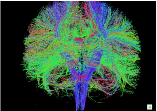
There are lots of different types of diffusion MRI including Diffusion Tensor Imaging (DTI) [Le Bihan et al., 2001], High angular resolution diffusion imaging (HARDI) [Tuch et al., 2002] and Diffusion spectrum magnetic resonance imaging (DSI) [Wedeen et al., 2008]. In this thesis,we mainly use DTI data to do analysis. DTI is a magnetic resonance imaging technique that enables the measurement of the restricted diffusion of water in tissue in order to produce neural tract images [Johansen-Berg and Behrens, 2013]. After a list of processing, tractography results could be extracted for every subject [Basser et al., 2000], as shown in Figure 1.4.

Figure 1.4: Diffusion MRI (Diffusion Tensor Imaging) tractography demonstration

1.2

Schizophrenia Brief Introduction

Schizophrenia is a mental disorder characterized by abnormal social behavior and failure to recognize what is real [Gottesman, 1991]. Common symptoms include false beliefs, unclear or confused thinking, hearing voices, reduced social engagement and emotional expression, and a lack of motivation [Kay et al., 1987]. Symptoms typically come on gradually, begin in young adulthood, and last a long time [First, 1994]. In this thesis,we tried to do some analysis on the schizophrenia effects on the brain.

Schizophrenia affects around 0.3% ∼0.7% of people at some point in their life [van den Heuvel et al., 2009]. The incidence is comparatively quite high and schizophrenia does affect our society. For example, the winner of the 1994 Nobel Prize for Economics and one of the best mathematician in our history, John Nash got schizophrenia and fight against it for around half a century.

A number of attempts have been made to explain the link between altered brain function and schizophrenia [Gottesman, 1991]. Studies using neuropsycholog-ical tests and brain imaging technologies to examine functional differences in brain activity have shown that differences seem to most commonly occur in the frontal lobes, hippocampus and temporal lobes [Kircher and Thienel, 2005]. Unfortunately,

the authentic understanding of schizophrenia is still in mystery [Andreasen et al., 2012].

1.3

Schizophrenia Effects on Brain

Optimal function of the human brain relies on the cooperation of constituent brain regions. The degree of cooperative activity between two brain regions at rest, mea-sured using functional connectivity [Friston, 1994], varies greatly across the brain. A complete lack of spatial variability in functional connectivity indicates that the entire brain is either acting as a single homogenous unit without regional special-ization, or the constituent brain regions are entirely asynchronous, without inte-gration. In contrast, optimum spatial variability in connectional strength reflects simultaneous integration and segregation across distributed brain regions. This di-versity forms the core of the overall topology of the complex functional architecture of human brain [Bullmore and Sporns, 2009][Tononi et al., 1994] altered in neu-ropsychiatric disorders such as schizophrenia [Alexander-Bloch et al., 2010][Fornito et al., 2012][Rubinov and Bullmore, 2013][van den Heuvel et al., 2013].

In healthy controls, presence of structural connectivity (putative axonal link-age assessed using diffusion tensor imaging) strongly predicts the strength of func-tional connectivity [Damoiseaux and Greicius, 2009][Honey et al., 2009][Skudlarski et al., 2010][van den Heuvel et al., 2009]. Nevertheless, most of the pairwise func-tional connections exist in the absence of a direct axonal linkage between two regions [Adachi et al., 2012][Damoiseaux and Greicius, 2009][Honey et al., 2009]. In general, functional links that have a structural basis are stronger and involve anatomically more proximal regions [Honey et al., 2009]. In contrast, functional links between regions that do not share direct axonal linkage appear to be weaker, and involve spatially distant regions [Adachi et al., 2012][Honey et al., 2009]. Functional links in the absence of one-to-one axonal connections may emerge from directed polysy-naptic connections or shared inputs/outputs involving a third region [Adachi et al., 2012]. Such indirect, weaker functional links may represent a connectional archi-tecture that is physiologically distinct from the links with a more direct structural basis.

Several studies observe a reduction in overall strength of functional con-nectivity in schizophrenia [Argyelan et al., 2014][Bassett et al., 2012][Lynall et al., 2010], while both increased [Skudlarski et al., 2010][Whitfield-Gabrieli et al., 2009] and decreased [Bluhm et al., 2007][Liang et al., 2006] connectivity involving dif-ferent regional connections are noted across the brain [Karbasforoushan and

Wood-ward, 2012][Pettersson-Yeo et al., 2011][Rubinov and Bullmore, 2013]. The presence of both hyper- and hypoconnectivity involving different regional connections [Guo et al., 2014][Skudlarski et al., 2010][Venkataraman et al., 2012][Woodward et al., 2012] indicates a large diversity in the distribution of connectivity across the func-tional links in schizophrenia. If such a diversification lies at the core of the dynamic pathophysiological process defining the presence of schizophrenia in an individual, then for a randomly chosen pair of brain regions, the connectional strength is likely to be less predictable in a patient compared to a healthy control.

Moreover, schizophrenia is characterized by the co-occurrence of positive, negative and cognitive symptoms [Rolls and Deco, 2010] which appear to be related to altered glutamatergic and GABAergic synaptic connectivity in several cortical areas [Coyle, 2006][Rolls, 2012][Rolls et al., 2008][Stan and Lewis, 2012]. Over the last two decades, much neuroimaging evidence for structural and functional deficits in the brain has strengthened the notion of dysconnectivity in schizophrenia [Friston and Frith, 1995][Frith, 1995]. The bulk of evidence for pathological dysconnectiv-ity in schizophrenia comes from functional Magnetic Resonance Imaging (fMRI) studies [Bluhm et al., 2007][Meyer-Lindenberg et al., 2005][Whitfield-Gabrieli et al., 2009][Zhou et al., 2007]. These numerous small to medium-sized studies have in-dicated that schizophrenia is unlikely to be a disorder of a single or small-set of functional connections. Instead, the emerging picture is suggestive of a widespread change in the brain’s network architecture, affecting the diversity (or complexity) that is characteristic of normal brain functions [Bassett et al., 2013][Lynall et al., 2010].

1.4

Functional Connectivity Entropy (FCE)

1.4.1 Functional Connectivity Entropy Origin

There is now a consensus that ageing is multifactorial; it is the joint outcome of genetics, the accumulation of random accidents and irreparable losses in molecular fidelity [Hayflick, 2007]. There is ample evidence that the genetic component alone plays a critical role in longevity determination [Christensen et al., 2006]. This is shown in regulatory and structural changes that occur with age in miRNA [Lanceta et al., 2010], mRNA [Rea and Johnson, 2003], ncRNA [Bates et al., 2009], protein expression [Morrow et al., 2004] and functional MRI [Zuo et al., 2010] in many species. Intuitively, these changes could be expected to correspond to changes in the functioning of the brain. But in what precise sense? This is the question we address in this work. The answer involves an explicitly quantitative way of characterizing

the intrinsic ageing process of the human brain.

We used entropy to quantify the functioning of the brain in individuals of different ages. Accordingly, we shall describe this as the functional connectivity entropy (FCE).

To motivate the definition of functional connectivity entropy, let us consider the following example of an analysis.

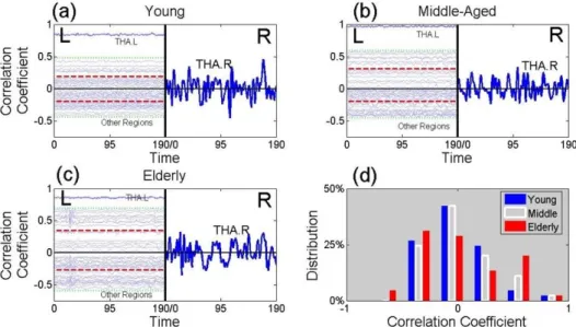
We parcellated the whole brain of three individuals into 90 regions, based on the AAL atlas [Tzourio-Mazoyer et al., 2002]. These were healthy males aged 24, 49 and 69 years, which we describe as ‘young’, ‘middle-aged’ and ‘elderly’. For these, we calculated the correlation coefficient between the BOLD signal of the thalamus in the right hemisphere and each of 45 brain regions in the left hemisphere (Table 2.2). These signals are represented in the left-hand of panels (a), (b) and (c) of Figure 1.5. Differences between the three individuals show up which are found in more extensive analyses.

The distribution of the correlation coefficients of the elderly male (red his-togram in Figure 1.5d) is more widely spread than that of the young male (blue histogram) and middle-aged male (white histogram). This leads to the elderly male having a larger functional connectivity entropy than that of the middle aged male, who has a yet larger functional connectivity entropy than that of the young male (see Figure 1.5d). This implies that the dispersion of correlations, between the right thalamus and a region of the brain in the left hemisphere, is typically an increasing function of age. This conclusion is found to hold in a full analysis, where a pairwise comparison of all regions in the brain is used, rather than just comparing regions in the left hemisphere with the right hemispheric thalamus.

Entropy characterizes the degree of underlying randomness of a random vari-able. Random variables with small entropies have a high level of predictability and hence a low level of randomness. By contrast, large entropies correspond to low levels of predictability and high levels of randomness [Vaseghi, 2008].

As outlined in Section 2.5, we view the brain as being divided (parcellated) into a number of distinct regions. For each pair of distinct brain regions, we cal-culated the correlation coefficient of their neuronal activity; this characterizes the functional coupling of the two brain regions. The resulting set of correlation coef-ficients generates a frequency distribution. The correlation coefficient of a distinct pair of brain regions, that have been randomly selected, can be regarded as a random variable that follows this frequency distribution. we use the dispersion or variability of this random variable as a measure of the functional connectivity entropy (c.f., complexity) of the neuronal dynamics of the brain.

Figure 1.5: The Origin of the Functional Connectivity Entropy

This figure presents time series from BOLD signals. The left-hand sides of panels (a), (b) and (c) contain 45 time series from brain regions of the left hemisphere. The vertical location of a time series, from a given brain region, is given by value of the correlation coefficient of that region with the right thalamus. Panel (a) is from a healthy young male (age 24 years), panel (b) is from a healthy middle-aged male (age 49 years) and panel (c) is from a healthy elderly male (age 69 years). The two horizontal red lines in panels (a), (b) and (c) give, separately, the mean over either positive or negative correlation coefficients. Thus the separation of these lines is a measure of the width of the distribution. In the right halves of panels (a), (b) and (c), the time series of the right thalamus is plotted (using a different vertical scale). Panel (d) gives a histogram of the correlation coefficients of the young male (in blue), the middle-aged male (in white) and the elderly male (in red).

The functional connectivity entropy effectively measures the dispersion (or spread) of functional connectivities that exist within the brain. we initiated this research under the assumption that the dispersion of functional connectivities is related to the age of the brain.

We collected fMRI data from 1248 individuals, ranging from 6 to 76 years of age. This provided a unique opportunity to characterize the ageing process of the human brain.

In the analysis of the fMRI dataset of differently aged individuals, we found that, at the population level, the functional connectivity entropy of the human brain has a definite tendency to increase over time. This can be viewed as there being a higher level of randomness in the way different brain-regions functionally interact with one another.

This section is modified from Yao et al. [2014].

1.4.2 Functional Connectivity Entropy in Schizophrenia

Most functional imaging studies in schizophrenia have predominantly focused on how the strength or magnitude of correlations between brain regions is affected in patients when compared to controls. Considering the overall variability in the con-nectional strength within the brain can capture significant amount of information on normal and abnormal brain function. we have shown that the information ob-tained using a measure of entropy predicts age-related changes to the connectional architecture of the brain [Yao et al., 2014]. Similarly, measuring the entropy of the functional connectivity dispersion can provide a systems neuroscience perspec-tive to the neurobiological basis of schizophrenia. Furthermore, most studies of large-scale networks in psychiatry have investigated abnormalities pertaining exclu-sively to connections surviving a specified correlation threshold, thus ignoring the weaker links. The shortcoming of such approaches was recently highlighted by Bas-sett et al. [2013], who showed that in a relatively small sample of 29 subjects with schizophrenia, the region-specific diversity of connectional strength and the state of organization of weak (rather than strong) connections were the crucial factors to discriminate patients with schizophrenia from controls.

The unpredictability of bivariate functional connectivity across the entire brain can be quantified using an index of entropy based on the principles of infor-mation theory (Shannon). Functional Connectivity Entropy (FCE) is a measure of randomness of the strength of functional connectivity, across all possible pairwise interregional connections in the brain [Yao et al., 2014]. This is different from the unpredictability or complexity across time that has been investigated previously in

schizophrenia [Bassett et al., 2012][Fernndez et al., 2013]. Higher FCE represents the presence of increased variability in connectional strength and has been observed in association with healthy ageing [Yao et al., 2014]. On the basis of a computational model, altered FCE has been attributed to a reduction in the pool of excitatory neurons [Yao et al., 2014], an observation that is highly relevant to the study of schizophrenia [Anticevic et al., 2013].

1.5

Hypothesis

Recent observations also suggest that weak (rather than strong) [Bassett et al., 2012] and long-distance (rather than short distance) functional links [Guo et al., 2014] are crucial to discriminate patients with schizophrenia from controls. This raises the possibility that the connectional architecture involving functional links that have no direct structural connectivity may be preferentially affected in schizophrenia.

In this thesis, we firstly showed the meanings of Functional Connectivity En-tropy (FCE). Afterwards, we represented the FCE property in schizophrenia. Then, we tested the hypothesis that the randomness of functional connectivity (measured using FCE) is abnormal in schizophrenia, and this abnormality is specific to func-tional links with no direct structural connectivity. we also investigated the rela-tionship between FCE and symptom burden in patients. Given its onset around adolescence, various dynamic changes coinciding with brain maturation take place in the initial few years in the course of schizophrenia, giving rise to several unstable and inconsistent neurobiological patterns that stabilized during the later stage of the illness [Pantelis et al., 2009]. In particular, the architecture of functional connec-tivity in patients is significantly affected by duration of illness. Patients with longer duration of illness show reduced segregation and integration [Liu et al., 2008], and reduced connectivity among core brain hubs [Collin et al., 2014]. In light of these observations, we expected a moderating effect of illness duration on FCE.

Chapter 2

Research Methodology

The information in Section 2.1, 2.2 and 2.11 have been also demonstrated in Yao et al. [2015], while those in Section 2.5.1, 2.7.1 and 2.8 have been mentioned in Yao et al. [2014].

2.1

Participants

This sample has been previously reported in a published article [Palaniyappan et al., 2013]. Thirty-four patients satisfying DSM-IV (Diagnostic and Statistical Manual of Mental Disorders) criteria for schizophrenia (n = 28) or schizoaffective disorder (n = 6) and thirty-two age, gender and parental socio-economic status [Rose and Pevalin, 2003] matched healthy controls were included. Patients were recruited from the community-based mental health teams (including Early Intervention in Psychosis teams) in Nottinghamshire and Leicestershire, UK. The diagnosis was made in a clinical consensus meeting in accordance with the procedure of Leckman et al. [1982], using all available information including a review of case files and a standardized clinical interview (SSPI) [Liddle et al., 2002]. All patients were in a stable phase of illness (defined as a change of no more than ten points in their Global Assessment of Function [GAF] score, assessed 6 weeks prior and immediately prior to study participation). The study was given ethical approval by the National Research Ethics Committee, Derbyshire, UK. All volunteers gave written informed consent. Clinical and demographic characteristics of this sample are presented in Table 2.1.

Patients were interviewed on the same day as the scan by a research psy-chiatrist and clinical severity of psychosis over the previous week was assessed on the basis of total SSPI scores. Duration of illness was estimated from the time of

reported onset of psychotic symptoms (Criterion A of DSM-IV schizophrenia), on the basis of information from case notes and clinical interview. The patient sample was divided into early-stage (<5 years duration) and later-stage (>5 years) illness, based on the clinical notion of ‘critical period’ of psychosis during which interven-tions can modify outcome [Crumlish et al., 2009][McGorry, 2002][Mcgorry et al., 2008] and clinical stability is achieved [Levie, 1979]. Thirty-two out of Thirty-four patients were receiving antipsychotic treatment at the time of scan. The chlorpro-mazine equivalent doses were calculated using data presented by Woods [2003] and Chong et al. [2000] (for clozapine). In addition, 25 mg risperidone depot injection every 14 days was considered equivalent to 4 mg oral risperidone per day, in accor-dance with the recommendation of the British National Formulary [Committee and of Great Britain, 2012].

Table 2.1: Clinical and demographic features

NS-SEC: National Statistics Socio-economic Classification CPZ equivalents: Chlorpromazine equivalents

This table is modified from Yao et al. [2015].

Patients (n=34) Controls (n=32) t/χ2_{, p} Age 34.1±9.1 33.4±9.1 t=0.30, p=0.76 Gender 25/9 22/10 χ2_{=0.18, p=0.67} Mean,parental NS-SEC (SD) 2.45±1.5 2.22±1.4 t=0.24, p=0.51 Handedness,(right/left) 29/5 28/4 χ2=0.07, p=0.79 SOFAS score 54.4±13.2 - -Antipsychotic,dose (CPZ equivalents) 694.5±715.8 -

-Median,duration of illness in years (range) 6.0(28) -

-Total,SSPI score 11.8±7.7 -

-2.1.1 Excluded subjects

The original sample consisted of 42 patients and 40 controls, but (3 patients, 5 controls) subjects were excluded due to movement artefacts in fMRI, 1 patient had poor quality DTI due to excessive movement, 2 patients aborted scans (1 DTI, 1 fMRI), and in 2 patients and 3 controls tractography was not successful due to image acquisition errors. There were no differences in the duration of illness (mean (SD) in years in the excluded group=8.9(4.5), included group=9.6(8.1), p=0.8), total SSPI score (mean (SD) in the included group=11.8(7.7), excluded group=11.6(6.2), p=0.94) or antipsychotic dose (mean (SD) in the excluded group=694.5(716), in-cluded group=485.7(357), p=0.46) between patients who were inin-cluded or exin-cluded in the analysis.

2.2

MRI Acquisition

Diffusion-weighted images were acquired using a single-shot, spin-echo, echo planar imaging (EPI) sequence in alignment with the anterior commissure - posterior com-missure (AC-PC) plane. The acquisition parameters were as follows: Repetition Time (TR) = 8.63 s, Echo Time (TE) = 56.9 ms, voxel size = 2mm isotropic, 112×

112 matrix, Field of View (FoV) = 224× 224×104, flip angle = 90o, 52 slices, 32 directions with a b-factor of 1000s/mm2, EPI Factor = 59, total scan time = 6.29 min.

For resting-state fMRI, 240 time points were acquired during the 10 minutes resting phase wherein the subjects were instructed to keep their eyes open and to relax, without the need to focus on any particular task. Dual-echo gradient-echo echo-planar images (GE-EPI) were acquired to enhance sensitivity, using 8-channel SENSE head coil (SENSE factor 2, anterior-posterior direction, TE1/TE2 25/53 ms, flip angle 85o, 255×255 mm field of view, in-plane resolution = 3 mm×3 mm, slice thickness = 4 mm, TR = 2500 ms; 40 descending axial slices, 240 time points per acquisition). Scans were inspected immediately after each acquisition, and if motion was detected, scans were repeated.

A magnetisation prepared rapid acquisition gradient echo image (MPRAGE T1) with 1 mm isotropic resolution, 256× 256× 160 matrix, TR/TE 8.1/3.7 ms, shot interval 3 s, flip angle 8o, SENSE factor 2 was also acquired for each participant for image registration and to define anatomical regions for tractography.

2.3

DTI processing

For DTI images, we first used FMRIB Software Library v5.0 (http://fsl.fmrib. ox.ac.uk/fsl) [Jenkinson et al., 2012] to remove the eddy-current and extract the brain mask from the B0 image. Then, we used TrackVis [Wang et al., 2007] to obtain the fiber images by the deterministic tracking method, with anatomical regions defined using the AAL convention [Tzourio-Mazoyer et al., 2002] (Table 2.2) on the basis of co-registered T1 image from each subject. This enabled us me to determine the presence of streamlines connecting every pair of brain regions. All the processes were performed using the PANDA suite [Cui et al., 2013].

If two brain regions A and B have one or more streamlines directly connecting each other, then this link AB is regarded as a direct or primary structural path. In contrast, if two brain regions X and Y have no direct connections, but share a direct connection with a common third region Z, then the link XY can be regarded as

indirect secondary structural path. If two brain regions K and L have neither direct connections, nor a common third region, but are connected to each other indirectly by virtue of being connected a common direct link (for example, K connects directly to A, A connects directly to B, B connects directly to L), then the link KL can be regarded as indirect tertiary structural path. To study the effect of the minimum streamline threshold, we varied the minimum from one to three and repeated the primary analysis (group comparisons). The results, shown in Section 4.5.3, indicated that the structural paths were robust across these thresholds.

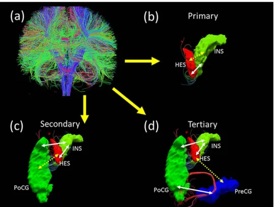
Thus, for every subject, we identified primary, secondary and tertiary paths on the basis of the DTI fiber streamlines. An illustration of these paths is shown in Figure 2.1.

Table 2.2: Names and abbreviations of AAL brain regions

Regions Abbr. Regions Abbr.

Amygdala AMYG Orbitofrontal cortex (middle) ORBmid

Angular gyrus ANG Orbitofrontal cortex (superior) ORBsup

Anterior cingulate gyrus ACG Pallidum PAL

Calcarine cortex CAL Paracentral lobule PCL

Caudate CAU Parahippocampal gyrus PHG

Cuneus CUN Postcentral gyrus PoCG

Fusiform gyrus FFG Posterior cingulate gyrus PCG

Heschl gyrus HES Precentral gyrus PreCG

Hippocampus HIP Precuneus PCUN

Inferior occipital gyrus IOG Putamen PUT

Inferior frontal gyrus (opercula) IFGoperc Rectus gyrus REC

Inferior frontal gyrus (triangular) IFGtriang Rolandic operculum ROL

Inferior parietal lobule IPL Superior occipital gyrus SOG

Inferior temporal gyrus ITG Superior frontal gyrus (dorsal) SFGdor

Insula INS Superior frontal gyrus (medial) SFGmed

Lingual gyrus LING Superior parietal gyrus SPG

Middle cingulate gyrus MCG Superior temporal gyrus STG

Middle occipital gyrus MOG Supplementary motor area SMA

Middle frontal gyrus MFG Supramarginal gyrus SMG

Middle temporal gyrus MTG Temporal pole (middle) TPOmid

Olfactory OLF Temporal pole (superior) TPOsup

Orbitofrontal cortex (inferior) ORBinf Thalamus THA

Orbitofrontal cortex (medial) ORBmed

2.3.1 Brain structural networks

In this thesis, we used diffusion tensor imaging (DTI), but not High angular resolu-tion diffusion imaging (HARDI) or diffusion spectrum magnetic resonance imaging (DSI) to detect structural connectivity. The main reason is that DTI images is eas-ier to be acquired with simpler requirement for sequence designing in MRI machine and shorter scanning time, compared with HARDI and DSI. Moreover, DTI

scan-Figure 2.1: Three types of structural paths defined using diffusion tractography (a): whole-brain fiber connection network construction by Diffusion Tensor Imag-ing data; (b): Heschl gyrus (HES) and Insula (INS) are directly connected with each other through white matter tracts. HES ↔ INS link is a primary structural path (c): Heschl gyrus and Postcentral gyrus (PoCG) are indirectly linked (discon-tinuous arrow) through white matter tracts (con(discon-tinuous arrows) that connect HES and PoCG with the Insula. Though there are no direct connections between HES and PoCG, INS acts as a common third region. HES ↔ PoCG link is termed as a secondary structural path. (d): Heschl gyrus and Precentral gyrus (PreCG) are indirectly linked (discontinuous arrow) through white matter tracts (continuous ar-rows) that connect HES with INS, INS with PoCG and PoCG with PreCG. There are no direct connections or a single common third region between HES and PreCG. HES↔PreCG link is termed as a tertiary structural path.

ning is comparatively technology with fewer noises [Johansen-Berg and Behrens, 2013] to get access to more reliable analysis. Thus, DTI images were chosen here to extract brain structural connectivity. The preprocessings of DTI imaging have been described in details in the last section, Section 2.3. We used streamline de-terministic tracking method to detect structural connectivity for it is simple and stable [Johansen-Berg and Behrens, 2013]. However, the streamline results some-times show large variances in the same link of different subjects [Savadjiev et al., 2008]. For some specific links, some subjects hold only several streamlines, while the others have hundreds of or even more than one thousand of streamlines in our data analysis. Thus, we used a binary network, but not the raw data to do analysis with a streamline threshold. The streamline threshold is ONE in the Results sections, which is also discussed in Section 4.5.3. We wrote a Matlab code to extract indirect pathways including secondary and tertiary links as described in the last section, Section 2.3, which is mainly based on matrix multiplication. Thus, we determined all primary, secondary and tertiary pathways for all brain connecitivies. It should be emphasized that all path calculations are based on structural (not functional) connectivity.

2.4

fMRI processing

Weighted summation of the dual-echo images produced a single set of low-artefact functional images [Posse et al., 1999]. Retrospective physiological correction was then performed [Glover et al., 2015]. The first five volumes of fMRI datasets were discarded, to allow for scanner stabilization. Further processing was then conducted by Statistical Parametric Mapping (SPM8) (http://www.fil.ion.ucl.ac.uk/spm) [Friston, 2007] and Data Processing Assistant for Resting-State fMRI (DPARSF) [Yan and Zang, 2010]. After slice-timing correction and realignment to the middle volume, the functional scans were spatially normalized using the unified segmenta-tion approach to a standard template (Montreal Neurological Institute) and resam-pled to 3×3 ×3 mm3. Data was then smoothed using a Gaussian kernel of 8 mm full-width at half- maximum, detrended, and then passed through a band-pass filter (0.01-0.08 Hz) to reduce low-frequency drift and high-frequency physiological noise. Nuisance covariates including head motion, global mean signals, white matter signals and cerebrospinal signals were regressed out from the time series. Regional time series were extracted in each of the 90 automated anatomical labelling atlas (AAL) [Tzourio-Mazoyer et al., 2002] based brain regions by averaging the signals of all voxels within a region. The names of the 90 brain regions are listed in Table

2.2, along with further details of fMRI preprocessing in Section 4.5.

2.4.1 Brain functional networks

After data preprocessing, the time series were extracted in each ROI by averaging the signals of all voxels within the region. The 90 regions were based on the AAL Template [Tzourio-Mazoyer et al., 2002]. After that, the Pearson’s correlation coef-ficient of every pair of regions was calculated. Since the atlas is the AAL template with 90 ROIs, 4005 functional connectivity links were obtained connecting every pair of regions. Thus a whole brain functional network was constructed.

2.5

Entropy Calculation

2.5.1 Functional Connectivity Entropy Meanings

We used entropy to quantify the functioning of the brain. Accordingly, we shall describe this as the functional connectivity entropy (FCE).

As outlined below, the brain was viewed as being divided (parcellated) into a number of distinct regions. For each pair of distinct brain regions, we calculated the correlation coefficient of their neuronal activity; this characterizes the functional coupling of the two brain regions. The resulting set of correlation coefficients gener-ates a frequency distribution. The correlation coefficient of a distinct pair of brain regions, that have been randomly selected, can be regarded as a random variable that follows this frequency distribution. we use the dispersion or variability (mea-sured using Shannon’s entropy, see below) of this random variable as a measure of the FCE (c.f., complexity) of the neuronal dynamics of the brain. we investigated, in this work, how this measure of the FCE changes with age and in Figure 2.2, we illustrated the behaviours of the brain’s dynamics that it captures.

Figure 2.2 (top row) shows the situation where every brain region fluctuates over time, but is totally correlated with all other regions. In such a case, the FCE of correlation coefficients is zero; all correlation coefficients are unity, and hence their distribution exhibits no randomness, just predictability. A case of non-zero FCE occurs when a range of different correlation coefficients are found between different pairs of brain regions. An example of this case is given by the second row in Figure 2.2. In the opposite case of completely independent or incoherent activity in all regions, the correlation coefficients will all be zero and their dispersion (FCE) will again be zero. This means the entropy measure is sensitive to co-ordinated activity that is most interesting, namely activity that is intermediate between fully

Figure 2.2: Illustration of the Functional Connectivity Entropy of the Brain In this figure, the brain is parcellated into a number of distinct regions. Different levels of brain activity (as measured by BOLD signals) are illustrated by different colors in the brain slices of the figure. we use two artificial data sets of BOLD signals to illustrate what the functional connectivity entropy captures about brain activity. Panels (a), (b) and (c) show brain activities of brain slices at three different times (T1, T2, T3), when the correlation coefficients between all regions of the brain are unity. In this case, all regions of the brain have the same color since they are be-having synchronously. Panel (d) shows the BOLD signals in different brain regions, for this case. Panel (e) shows the corresponding distribution of the correlation co-efficients (a ‘spike’ located at a correlation coefficient of unity). The functional connectivity entropy for this case is zero (the minimum possible value).

Panels (f), (g) and (h) show the brain activities at three different times (T1, T2, T3), when all correlation coefficients are generally different (so all regions have dif-ferent colors, indicating that all regions are behaving asynchronously. Panel (i) shows BOLD signals in different brain regions, for this case. Panel (j) shows the corresponding distribution of the correlation coefficients (a uniform distribution). The functional connectivity entropy in this case is the maximum possible value. This figure is reproduced from Yao et al. [2014].

synchronised and fully incoherent brain-region dynamics.

2.5.2 Functional Connectivity Entropy Calculation Method

After data preprocessing, the time series were extracted in each ROI by averaging the signals of all voxels within the region. The 90 regions were based on a selected atlas, say the AAL Template. After that, we calculated the Pearson Correlation Coefficient of every pair of regions. Since the atlas was the AAL template, we had 4005 function links connecting every two regions. Thus we constructed a whole brain functional network.

Given 4005 different correlation numbers, we considered the values of the correlation coefficients as a realization of a random variable. The range of this was [-1,1]. we then defined the brain functional connectivity entropy as the relative

en-tropy, i.e., the KL (Kullback-Leibler) divergence from the correlation distribution to a reference Lebesgue measure. In practice, we did not have a continuous distri-bution of correlation coefficients, but 4005 correlations values from each individual. we thus separated all 4005 realizations into 20 class intervals of equal width, and determined the frequency (pi) of each class. These frequencies were used to calculate the Shannon entropy (sum of -pi*log(pi)) of the whole brain. This can be considered as the functional connectivity entropy (FCE).

2.6

Statistical inference

We applied linear regression model [Seber and Lee, 2012] to remove age, sex and dose effects for patients and controls, which was applied in Figure 3.10, 3.11, 4.2 and 4.3. We used Cohen’s d [Cohen, 1992] to quantify the effect size of the mean differences.

2.7

Computational Model

2.7.1 Computational model of brain networks

A computational model from Deco et al.’s work [Deco and Jirsa, 2012] could be used to verify the results about functional connectivity entropy.

Neuron dynamics

The global structure of the model is illustrated in Figure 2.3. Every brain region served as a node in a large scale network, which consists of a population of excitatory pyramidal neurons and a population of GABAergic inhibitory neurons, which are all-to-all connected. The communication between every two nodes is through synaptic connections between excitatory neurons in those areas.

For each brain area, an integrate-and-fire neuron model with excitatory (AMPA and NMDA) and inhibitory (GABA) synaptic receptors was applied. The dynamics of the membrane potentialV(t) are described by:

   CmdV_d(_tt) =−gm(V(t)−VL)−Isyn(t), V(t)< Vthr, V(t) =Vreset, V(t)≥Vthr. (2.1)

The total synaptic currentIsyn is given by the sum of glutamatergic AMPA

NMDA (IN M DA,REC) recurrent excitatory currents, and GABAergic recurrent

in-hibitory currents (IGABA):

Isyn=IAM P A,ext+IAM P A,rec+IN M DA,rec+IGABA, (2.2)

where,                IAM P A,ext(t) =gAM P A,ext(V(t)−VE)Pjs AM P A,ext j (t), IAM P A,rec(t) =gAM P A,rec(V(t)−VE)P_jωAM P Aj s AM P A,rec j (t), IN M DA,rec(t) = gN M DA,rec(V(t) −VE) 1+γe−βV(t) P jωjN M DAs N M DA,rec j (t), IGABA(t) =gGABA(V(t)−VI)P_jωGABAj sGABAj (t),

(2.3)

The gating variablessj(t) are the fractions of open channels of neurons and

are given by:

                       dsAM P A,ext_j (t) dt =− sAM P A,ext_j (t) τAM P A + P kδ(t−tkj), dsAM P A,rec_j (t) dt =− sAM P A,rec_j (t) τAM P A + P kδ(t−tkj), dsN M DA,rec_j (t) dt =− sN M DA,rec_j (t) τN M DA,decay +αx N M DA,rec j (t)(1−s N M DA,rec j (t)), dxN M DA,rec_j (t) dt =− sN M DA,rec_j (t) τN M DA,rise + P kδ(t−tkj), dsGABA j (t) dt =− sGABA j (t) τGABA + P kδ(t−tkj), (2.4)

The sums over thekindex represent all of the spikes emitted by presynaptic neuronj (at timestk_j). The description and value of most parameters are shown in Table 2.3.

Each local area contains 100 excitatory neurons and 100 inhibitory neu-rons. The connection strengths between and within the populations are determined by dimensionless strength ω. Illustrated in Figure 2.3, there are 4 different intra-connection strength: 1 excitation (AMPA and NMDA) within excitatory neurons

ω1; 2 excitation (AMPA and NMDA) from excitatory neuron to inhibitory neuron

ω2 = 1; 3 inhibition (GABA) from inhibitory neuron to excitatory neuronω3 = 1; 4

inhibition (GABA) within inhibitory neurons ω4 = 1. we vary ω1 systemat-ically to see the implications for the global functional connectivity entropy. The inter-regional connection strengthωinter is proportional to number of fibers linking every two regions. The neuroanatomical matrix whose element is fiber number, is obtained by Diffusion Tensor Imaging. Here, we used averaged structural matrix

from 46 healthy people, which is showed in Figure 2.4.

All neurons always received an external background input fromNext = 800

external neurons emitting independent Poisson spike trains at a rate of 3Hz. More specifically, for all neurons inside a given population p, the resulting global spike train, which is still Poissonian, had a time-varying rateν_extp (t), governed by,

τn dν_extp (t) dt =−(ν p ext(t)−ν0) +σ √ 2τnξp(t), (2.5)

whereτn = 300ms, ν0 = 2.4kHz, σν = 0.2 is the standard deviation of νextp (t), and ξp(t) is normalized Gaussian white noise.

Table 2.3: Neural and synaptic parameters

Excitatory neuron Inhibitory neuron

Membrane capacitanceCm 0.5 nF 0.2 nF Excitatory reversal potentialVE 0 mV Leak conductancegm 25 nS 20 nS Inhibitory reversal potentialVI -70 mV

Resting potentialVL -70 mV -70 mV Decay timeτAM P A 2 ms

Threshold potentialVthr -50 mV -50 mV Rise timeτN M DA,rise 2 ms Reset potentialVreset -55 mV -55 mV Decay timeτN M DA,decay 100 ms

Refractory timeτref 2 ms 1 ms Decay timeτGABA 10 ms

Synaptic conductance gAM P A,ext 2.496 nS 1.944 nS α 0.5 kHz gAM P A,rec 0.104 nS 0.081 nS β 0.062 gN M DA,rec 0.327 nS 0.258 nS γ 0.28 gGABA 2.45 nS 1.2 nS BOLD signal

The simulation of the fMRI BOLD signal is computed by means of the Balloon-Windkessel hemodynamic model Friston et al. [2003]. The BOLD-signal of each region is driven by the level of neuronal activity summed over all neurons in both populations (excitatory and inhibitory populations) in that particular region. In all simulations, neuronal activity is given by the rate of spiking activity in a time window of 1 ms. In brief, for thei’th region, neuronal activityzi causes an increase

in a vasodilator signal si that is subject to autoregulatory feedback. Inflow fi

responds in proportion to this signal with concomitant changes in blood volumeνi

and deoxyhemoglobincontentqi. The equations relating these biophysical variables

are:                dsi(t)) dt =εizi−kisi−γi(fi−1), dfi(t) dt =si, τidν_di(_tt) =f i−νi1/α, τidq_di(_tt) = fi[1 −(1−ρi)1_/fi] ρi − qiνi1/α νi , (2.6)

Figure 2.3: Schematic representation of the brain network

Each brain area is comprised of excitatory neurons (red triangles) and inhibitory interneurons (blue circles). 1234 represent the four different intra-connection during each brain area, and 5describes the inter-connection between different brain area, which depends on DTI.

Figure 2.4: Neuroanatomical connectivity matrix

Neuroanatomical connectivity matrix, obtained by DTI after averaging across 46 human subjects.

be a static nonlinear function of volume and deoxyhemoglobin that comprises a volume-weighted sum of extra- and intravascular signals:

yi =V0[7ρi(1−qi) + 2(1− qi νi

) + (2ρi−0.2)(1−νi)], (2.7)

where V0 = 0.02 is the resting blood volume fraction. The biophysical parameters

were taken asεi= 0.2,ki = 0.65,γi = 0.41,τi= 0.98, α= 0.32ρi = 0.34.

Simulation of the functional connectivity entropy

After the simulated BOLD time series were obtained, the global signal (average over all regions) was regressed out. Figure 2.5 shows typical temporal evolution of the simulated BOLD signal (after regression) for several brain regions. we then calcu-lated the simucalcu-lated functional connectivity by calculating the correlation matrix of the BOLD time series. Figure 2.6 and 2.7 plot an example of stimulated functional connectivity matrix and corresponding distribution of correlation, respectively. Us-ing the calculation method of functional connectivity entropy, we could compare the simulated functional connectivity entropy with that from fMRI data.

When we increase intra-excitatory connection strength ω1 with other pa-rameters fixed, the firing rate of excitatory neurons in the whole brain increase. (Firing-rate amplification of inhibitory neurons can be ignored compared to that of excitatory neurons.) Based on the fact that the firing rate of one excitatory neuron, in resting state, is about 3Hz and that the model of one neuron here could also described the dynamics of several neurons or a neuron mass, we can calculate the actual excitatory neuron number in each brain region by the 100 times mean firing rate divided by 3Hz. (Here we just use the averaged firing rate of all excitatory neurons in the whole brain, not in each brain region.) Figure 2.8 illustrates the positive correlation between actual excitatory neuron number and intra-excitatory connection strength. The two red dashed lines show the range of connection strength [1.78,1.81], which makes the corresponding entropy match the human data. Based on the least squares line (black dashed line), the neuron number range is limited to [888,1130] (indicated by green text arrows).

2.7.2 Computational model in Schizophrenia

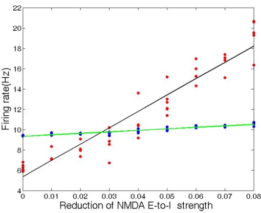
When we reduced the excitatory NMDA connection strength from the excitatory population to the inhibitory population within each brain region with the other parameters fixed, the firing rate of the excitatory neurons averaged across the whole brain increased, as illustrated in Figure 2.9.

Figure 2.5: Simulated BOLD signals

Simulated BOLD signal for thalamus (blue), Inferior temporal gyrus (red) and In-sula(green) when intra-excitatory connection strengthω1_=1.81.

Figure 2.6: Simulated functional connectivity matrix

Simulated functional connectivity matrix when intra-excitatory connection strength

Figure 2.7: The distribution of correlation coefficients

The distribution of correlation coefficients when the intra-excitatory connection strengthω1=1.81.

Figure 2.8: Excitatory neuron number versus intra-excitatory connection strength

ω1

When we reduced the excitatory NMDA connection strength from all excita-tory neurons (i.e. E-to-E and E-to-I, where E indicates excitaexcita-tory and we indicates inhibitory) by 8%, the firing rate of the excitatory neurons averaged across the whole brain decreased by 50%.

2.8

Methods for Functional Connectivity Entropy

Ori-gin: Ageing Problem (Section 3.1)

2.8.1 Subjects

Our meta-analysis included 26 datasets, with a total of 1248 samples. These covered a range of individuals from 6 to 76 years of age. Samples of poor quality were excluded.

Note that 22 of these datasets came from the 1000 Functional Connec-tomes Project (http://fcon_1000.projects.nitrc.org/), where data came from all over the world including China, Britain and United States. In these 22 data sets, there were 842 samples, with ages ranging from 18 to 73 years, with 357 of them male. The mean age was 28.3±12.3 years. Details are listed in Table 2.4. The fMRI scans performed by 1000 Functional Connectomes Project were carried out in accordance with the guidelines issued by the local ethical committees of the various

Figure 2.9: Average firing rate versus percent reduction of NMDA strength from the excitatory to inhibitory (E-to-I) population

Here red and blue dots represent different trials for excitatory and inhibitory neu-rons, respectively. The black and green lines are the corresponding least-squares fit. The linear correlation between the excitatory firing rate and the connection strength is statistically significant (10−20), while this is not the case for the inhibitory neu-rons.

research institutes, which can be found in their website. And informed consent was obtained from all subjects.

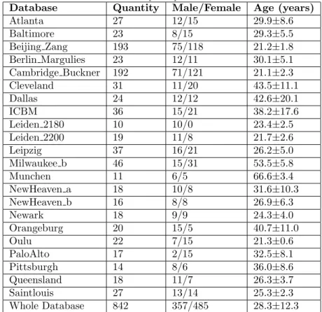
Table 2.4: Detailed information of 22 databases from the FCON 1000 Project This table is modified from Yao et al. [2014].

Database Quantity Male/Female Age (years)

Atlanta 27 12/15 29.9±8.6 Baltimore 23 8/15 29.3±5.5 Beijing Zang 193 75/118 21.2±1.8 Berlin Margulies 23 12/11 30.1±5.1 Cambridge Buckner 192 71/121 21.1±2.3 Cleveland 31 11/20 43.5±11.1 Dallas 24 12/12 42.6±20.1 ICBM 36 15/21 38.2±17.6 Leiden 2180 10 10/0 23.4±2.5 Leiden 2200 19 11/8 21.7±2.6 Leipzig 37 16/21 26.2±5.0 Milwaukee b 46 15/31 53.5±5.8 Munchen 11 6/5 66.6±3.4 NewHeaven a 18 10/8 31.6±10.3 NewHeaven b 16 8/8 26.9±6.3 Newark 18 9/9 24.3±4.0 Orangeburg 20 15/5 40.7±11.0 Oulu 22 7/15 21.3±0.6 PaloAlto 17 2/15 32.5±8.1 Pittsburgh 14 8/6 36.0±8.6 Queensland 18 11/7 26.3±3.7 Saintlouis 27 13/14 25.3±2.3 Whole Database 842 357/485 28.3±12.3

Another 2 datasets were from the ADHD-200 Consortium for the global com-petition (http://fcon_1000.projects.nitrc.org/indi/adhd200/). One of these was from the Phyllis Green and Randolph Cowen Institute for Pediatric Neuro-science at the Child Study Center, New York University Langone Medical Center, New York, New York and the Nathan Kline Institute for Psychiatric Research, Or-angeburg, NY, USA. The other came from the Institute of Mental Health, Peking University and the National Key Laboratory of Cognitive Neuroscience and Learn-ing, Beijing University. Since they were both concerned about ADHD classification, their data were ADHD patients versus controls (normal individuals). we cannot apply the data from individuals with ADHD disorder, since their brains may be different from normal people, and we used only the controls, namely the normal people from the 2 datasets. In total, there were 241 samples, with 134 of them male. Their mean age was 11.83±2.47 years, so they were teenagers/children. Since most samples in the other dataset were more than 18 years old, we selected the two

datasets to complete the analysis about ageing in the range of 6 years to 18 years old. The fMRI study in Peking University was approved by the Research Ethics Review Board of Institute of Mental Health, Peking University. Informed consent was also obtained from the parent of each subject and all of the children agreed to participate in the study. The fMRI scans from NYU were carried out in accordance with the guidelines issued by the local ethical committee, and informed consent was obtained from all subjects.

There was also one dataset of elderly people, covering 117 samples from the Department of Psychiatry, Tongji Hospital, Tongji University School of Medicine and Department of Biological Psychiatry, Shanghai Mental Health Centre, Shang-hai Jiao Tong University School of Medicine. In this dataset, 73 were male. The mean age was 70.42±3.52 years. With a designed health status checklist, we ex-cluded individuals with: obvious cognitive decline, a diagnosis of AD, serious func-tional decline (having difficulty with independent living), as well as individuals with major medical or psychiatric conditions such as cancer, current chemotherapy/ra-diation treatment, major depression, and schizophrenia. This study was approved by the Human Research Ethics Board of Tongji Hospital in Shanghai, China and all participants gave written informed consent before being enrolled in this part.

The last dataset was from the Department of Biomedical Imaging and Ra-diological Sciences, National Yang-Ming University, Taipei, Taiwan and the Brain Connectivity Laboratory, Institute of Neuroscience, National Yang-Ming University, Taipei, Taiwan. There were 48 samples in the dataset. All were male and covered a range of ages from 21 to 76 years. The mean age was 43.8±17.0 years and all indi-viduals were normal and healthy. Moreover, the T1-image and DTI data of these 48 samples were also applied in this thesis. The fMRI scans from National Yang-Ming University were carried out in accordance with the guidelines issued by the local ethical committee, and informed consent was obtained from all subjects.

2.8.2 Data Acquisition

The various ways that data were acquired in the 22 datasets from the 1000 Functional Connectomes project can be found in their website,http://fcon_1000.projects.

nitrc.org/. Moreover, the acquisition of the two datasets from the ADHD-200

Consortium for the global competition was in their website, http://fcon_1000.

projects.nitrc.org/indi/adhd200/.

In the dataset from Shanghai, all people underwent functional scanning using a Siemens Trio 3T scanner at East China Normal University, Shanghai, China. Foam padding was used to minimize head motion for all subjects. Functional images

were acquired using a single-shot, gradient-recalled echo planar imaging sequence (repetition time = 2000 ms, echo time = 25 ms and flip angle = 90 degrees). Thirty-two transverse slices (field of view = 240 × 240 mm2_{, in-plane matrix = 64 × 64,}

slice thickness = 5 mm, voxel size = 3.75 × 3.75 × 5 mm3), aligned along the anterior commissureCposterior commissure line were acquired. For each subject, a total of 155 volumes were acquired, resulting in a total scan time of 310s. Subjects were instructed simply to rest with their eyes closed, not to think of anything in particular, and not to fall asleep.

At last, in the dataset from Taiwan, all people underwent structural, func-tional and diffusion tensor imaging scanning using a Siemens Trio 3T scanner at Na-tional Yang-Ming University, Taiwan. Foam padding was used to minimize head mo-tion for all subjects. Funcmo-tional images were acquired using a single-shot, gradient-recalled echo planar imaging sequence (repetition time = 2500 ms, echo time = 27 ms and flip angle = 77). Fourty-three transverse slices (field of view = 220× 220 mm2, in-plane matrix = 64 × 64, slice thickness = 3.4 mm, voxel size = 3.44 ×

3.44×3.4 mm3), aligned along the anterior commissureCposterior commissure line were acquired. For each subject, a total of 200 volumes were acquired, resulting in a total scan time of 500s. Subjects were instructed simply to rest with their eyes closed, not to think of anything in particular, and not to fall asleep. The dif-fusion tensor images covering the whole brain were obtained using spin echo-based echo planar imaging sequence, including 30 volumes with diffusion gradients applied along 30 non-collinear directions (b = 1000 s/mm2) and three volumes without dif-fusion weighting (b = 0 s/mm2_{). Each volume consisted of 63 contiguous axial slices}

(repetition time = 11000 ms, echo time = 104 ms, flip angle = 90 degrees, field of view = 100 × 100 mm2, matrix size = 128 × 128, voxel size = 2 × 2 × 2 mm3). To improve the signal to noise ratio, the entire sequence was repeated three times. Subsequently, high-resolution T1-weighted anatomical images were acquired in the sagittal orientation using a magnetization-prepared rapid gradient-echo sequence (repetition time = 3500 ms, echo time = 3.5 ms, flip angle = 7, field of view = 256

×256 mm2, matrix size = 256 ×256, slice thickness = 1 mm, voxel size = 1×1×

1 mm3 and 192 slices)on each sub