FutureWater
The added value of high-resolution above
coarse-resolution remote sensing images in
crop yield forecasting
A case study in the Egyptian Nile Delta
December 2012
Authors Wilco Terink Peter Droogers Jos van Dam Gijs Simons Maurits Voogt
Report FutureWater: 116
This document is produced by the CGIAR Research Program on Climate Change, Agriculture and Food Security (CCAFS), which is a strategic partnership of CGIAR and Future Earth. The views expressed in this document cannot be taken to reflect the official opinions of CGIAR or Future Earth.
Executive summary
Crop growth models play a major role in sustaining the world-wide food security. These models are used to simulate crop growth during the growing season, and the final crop yield at the end of the growing season, given the farmers’ management practices. At a more strategic level, these crop growth models play an important role to decision makers to take timely decisions regarding food import and/or export strategies. The simulation accuracy of crop growth models relies on the quality of the input data. Since crop yield forecasting applications are often applied over large areas that rely on a spatially distributed crop growth model, the uncertainty in the spatial variation of the input data increases. Remote sensing images are often used in crop growth models because remote sensing images provide spatially distributed input data to these models. These images are available in numerous spatial resolutions, where coarse resolution images are often freely available compared to the more expensive high-resolution images. Therefore, the objective of the current study was to evaluate the added value of high-resolution satellite imagery above coarse-resolution satellite imagery in crop yield forecasting.
The current study focuses on a small area (240 x 240 m) in the Nile Delta in Egypt. In this area two crops are grown during winter season, being wheat and berseem. Besides these main crops, the area consists of some build-up area and a minor other crop. For the coarse-resolution simulation, a synthetic MODIS pixel (240 x 240 m) was created using bilinear interpolation of high-resolution ASTER imagery (15 x 15 m). The ASTER imagery was used for the high-resolution simulations. For the coarse-resolution simulation one bi-weekly time-series of remotely sensed LAIs was used, and for the high-resolution simulations 256 bi-weekly time-series of remotely sensed LAIs were used. These LAIs were used as input to the Soil-Water-Plant-Atmosphere (SWAP) model to simulate crop yields. Yields were simulated both for wheat and berseem. Actual yields were calculated in two steps: first the relative yield is calculated with the Soil-Water-Plant-Atmosphere (SWAP) model, which is based on the reduction in potential transpiration. Second, the actual crop yield is calculated by multiplying the relative yield with the potential yield. Before crop yield forecasting was done, the SWAP model was calibrated for wheat and berseem separately. SWAP was calibrated for a representative wheat and berseem pixel, matching the bi-weekly derived SEBAL actual evapotranspiration. Calibration results were satisfactory, with an R2 of 0.90 for wheat and an R2 of 0.89 for berseem.
To evaluate the added value of high-resolution above coarse-resolution satellite imagery in crop yield forecasting, three simulations were defined:
Reference run: this represents the “real” crop yield situation in the field. In other words, this data set is the observed data as would have been measured during that growing season. In this run SWAP is driven with the high-resolution ASTER LAIs throughout the entire growing season. This includes the forecasting period (last two months) and the period before the forecasting period.
High-resolution run: for this run the high-resolution ASTER LAIs is used up till the forecasting period. For the forecasting period no remotely sensed LAI is available. Therefore, SWAP was driven with ‘standard values’ for LAI during this period. For the ‘standard values’ the MODIS LAI was used.
Coarse-resolution run: for this run the coarse-resolution MODIS LAI is used up till the forecasting period. For the forecasting period, the same ‘standard values’ were used as for the high-resolution forecasting period.
It was concluded that a farmer can obtain a much more accurate yield forecast if high-resolution satellite imagery is used. If coarse-resolution remote sensing would have been used, then for
wheat the yield is overestimated with approximately 9%, and for berseem with 26%. If high-resolution satellite imagery will be used, then the forecast accuracy is much better; wheat underestimated with 1.4% and berseem overestimated with 2.1%. The use of high-resolution remote sensing enables the farmer to optimize his local specific farm and water management. This means that irrigation applications are more accurate under the use of high-resolution imagery. This is especially true for berseem, where the reference situation shows that 442 m3/ha is really required. Based on the best estimate (high-resolution remote sensing) 486 m3/ha is applied (10% overestimated), while under coarse-resolution satellite imagery zero irrigation is applied (100% error). For wheat the reference situation shows that 1148 m3/ha is really
required. Under high-resolution remote sensing, the applied amount of irrigation is 1093 m3/ha, which is a slight underestimation (~5%), while under coarse-resolution remote sensing 1194 m3/ha is applied, which is a slight overestimation (~4%).
At a more strategic level, decision makers will have considerable advantages if high-resolution remote sensing is used in crop yield forecasting; they can better take timely decisions regarding food import and/or export strategies. It was concluded that a significant amount of money can be saved if high-resolution remote sensing is used in crop yield forecasting. If coarse-resolution remote sensing is used in crop yield forecasting for wheat, then approximately 250 million US$ is lost through less export due to overestimated wheat yields. High-resolution remote sensing for wheat would lead to underestimated wheat yields, meaning that decision makers import too much wheat for a price of approximately 100 million US$. Losses are even more significant for berseem. Both coarse- and high-resolution remote sensing results in overestimated berseem yields. If coarse-resolution remote sensing will be used for berseem, then 3.2 billion US$ is lost through less exports, whereas high-resolution leads to a loss of approximately 0.3 billion US$. It was concluded that costs for the use of high-resolution remote sensing are negligible small compared to these benefits, and therefore it is well-worth investing in high-resolution remote sensing images.
The results of the current study provide some interesting perspectives for future studies:
1. It would be interesting to conduct the study over a larger area, using many coarse-resolution MODIS images and high-coarse-resolution ASTER images. This will lead to increased model input uncertainties (more crops);
2. The current study used a representative MODIS pixel (MODISr). If a real MODIS pixel
would have been used, then results as presented in this study will be different. Since the interpolated high-resolution images (MODISr) are more accurate than a real MODIS
pixel, the differences between high- and coarse-resolution satellite imagery in crop yield forecasting may be even larger than presented in the current study. This means that the benefits from high-resolution imagery in crop yield forecasting will be larger. As a follow-up, it is therefore recommended to use real MODIS satellite imagery;
3. It is interesting for a follow-up to experience with the use of high- vs. coarse-resolution remote sensing during various growing stages. Also a different length for the
forecasting period would be an interesting assessment;
4. Improved forecasting methods can be considered where focus should be on model selection as well as on data assimilation approaches;
Table of contents
1 Introduction 7
1.1 Background 7
1.2 Objective 8
2 Focal area – Egyptian Nile Delta 9
2.1 Area and pixel selection 9
2.2 Wheat and berseem yields 10
2.3 Overview 11
3 Data and methodology 14
3.1 Field data 14
3.1.1 Cropping patterns 14
3.1.2 Yields 14
3.2 Remote sensing and SEBAL 15
3.2.1 Available and selected satellite data 15
3.2.2 The SEBAL approach – theory and model setup 16
3.2.3 Harvest Index and biomass 19
3.3 Simulation modeling 19
3.3.1 SWAP description 19
3.3.2 Data and model schematization 21
3.3.3 SWAP calibration and validation 27
3.4 Crop yield forecasting 35
4 Results 37
4.1 Total yield and irrigation 37
4.2 Spatial variation 38
4.3 Temporal variation 42
5 Discussions and implications 44
5.1 Relevance 44
5.2 Overview of results 45
5.2.1 Advantage for farmers 45
5.2.2 Advantage for decision makers 45
5.3 Cost of forecasting 47
5.4 Future outlook 47
Tables
Table 1: Egypt country statistics (source: World Bank). ... 12
Table 2: Water resources and sectorial demand in the Meet Yazid command area (source: MALR, 2010). ... 13
Table 3: Overview of available satellite imagery per period (bi-weekly). ... 15
Table 4: Derived SWAP soil-physical parameters. ... 24
Table 5: Schematization of the SWAP soil profile. ... 24
Table 6: Calibration parameters and resulting calibrated values for wheat. ... 28
Table 7: Calibration parameters and resulting calibrated values for berseem. ... 30
Table 8: Calibration and validation statistics for wheat and berseem. ... 34
Table 9: Water balance for the calibrated wheat (left table) and berseem (right table) pixel. .... 35
Table 10: Summary of the satellite imagery used during the first period and the forecasting period. ... 35
Table 11: Final wheat and berseem yields for the reference situation, and the high- and coarse-resolution runs. Also the errors with respect to the reference situation are shown. ... 37
Table 12: Total irrigation gift during the forecast period for the reference situation and the high- and coarse-resolution runs. Also errors with respect to the reference situation are shown. ... 38
Table 13: Wheat yield, production price and total production for the entire country for the reference situation and forecast based on coarse- and high-resolution remote sensing. ... 46
Table 14: Berseem yield, production price and total production for the entire country for the reference situation and forecasting based on coarse- and high-resolution remote sensing. ... 46
Figures
Figure 1: Meet Yazid command area (red diagonal lines) in the Egyptian Nile Delta. The green dot represents the Baltim meteorological station used in the current study. ... 10Figure 2: A high-resolution 5 m IKONOS image (of a different year) with the selected 240 m coarse-resolution image (yellow box) superimposed, to illustrate how the 240 m pixel size relates to individual field sizes. ... 10
Figure 3: Wheat yield in Egypt, Libya, and Sudan for the period 1961-2010 (source: FAOSTAT). ... 11
Figure 4: Average monthly rainfall and temperature for Egypt from 1990-2009 (source: World Bank). ... 12
Figure 5: Rainfall and reference evapotranspiration (ETref) in the Nile Delta, Egypt (source: Baltim meteorological station and eLeaf). ... 13
Figure 6: High-resolution pixel classification within the selected coarse-resolution pixel. ... 14
Figure 7: Typical examples of some ASTER images of the winter growing season. ... 16
Figure 8: Schematic view of the SEBAL algorithm. ... 17
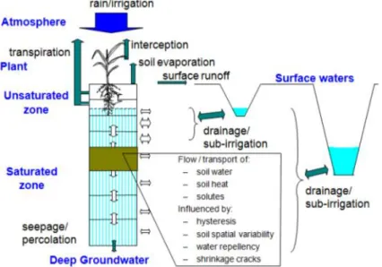
Figure 9: SWAP model domain and transport processes (van Dam, 2000). ... 20
Figure 10: Schematization of the SWAP model (van Dam, 2000). ... 21
Figure 14: Reduction coefficient for root water uptake, αw as function of soil water pressure
head h and potential transpiration rate Tp (Feddes et al., 1978). ... 25
Figure 15: Typical partitioning of assimilated dry matter among leaves, stem, roots and storage organs as function of development stage (Van Dam, 2000). ... 26 Figure 16: Boxplot of SEBAL actual evapotranspiration (ETa) for all high-resolution wheat pixels during the growing season (period 1-14). The colored lines represent a selection of individual wheat pixels. Periods are defined as two-weekly periods. ... 29 Figure 17: Boxplot of SEBAL actual evapotranspiration (ETa) for all high-resolution berseem pixels during the growing season (period 1-14). The colored lines represent a selection of individual berseem pixels. Periods are defined as two-weekly periods. ... 30 Figure 18: Actual observed and simulated evapotranspiration for wheat. Results are shown for each 14-day period for both the uncalibrated and the calibrated wheat pixel with ID 87. ... 31 Figure 19: Scatter-plot of observed versus simulated actual evapotranspiration for wheat pixel with ID 87. Both the uncalibrated and calibrated results are shown. ... 31 Figure 20: Actual observed and simulated evapotranspiration for wheat. Results are shown for each 14-day period for the validated wheat pixel with ID 170. ... 32 Figure 21: Scatter-plot of observed versus simulated actual evapotranspiration for wheat. Results are shown for the validated wheat pixel with ID 170. ... 32 Figure 22: Actual observed and simulated evapotranspiration for berseem. Results are shown for each 14-day period for both the uncalibrated and the calibrated berseem pixel with ID 22. . 33 Figure 23: Scatter-plot of observed versus simulated actual evapotranspiration for berseem pixel with ID 22. Both the uncalibrated and calibrated results are shown. ... 33 Figure 24: Actual observed and simulated evapotranspiration for berseem. Results are shown for each 14-day period for the validated berseem pixel with ID 63. ... 34 Figure 25: Scatter-plot of observed versus simulated actual evapotranspiration for berseem. Results are shown for the validated berseem pixel with ID 63. ... 34 Figure 26: Illustration of the use of LAIs in the three runs which are compared in the current study. The last four two-weekly periods (2 months) are used as the forecasting period. ... 36 Figure 27: Spatial variation in relative yields at the end of the growing season for the reference situation (top left), high-resolution run (top middle), and coarse-resolution run (top right). The bottom plots represent the errors of the high- and coarse-resolution runs with respect to the reference run. ... 39 Figure 28: Spatial variation in total irrigation gifts during the forecast period for the reference situation (top left), high-resolution run (top middle), and coarse-resolution run (top right). The bottom plots represent the errors of the high- and coarse-resolution runs with respect to the reference run. ... 40 Figure 29: LAI for the coarse-resolution run, the average of the high-resolution wheat pixels, and selected wheat pixels where the irrigation gift is underestimated in the high-resolution run. ... 41 Figure 30: LAI for the coarse-resolution run, the average of the high-resolution wheat pixels, and selected wheat pixels where the irrigation gift is overestimated in the high-resolution run. 41 Figure 31: LAI for the coarse-resolution run and the average of the high-resolution berseem pixels. ... 42 Figure 32: Boxplots that represent per period (bi-weekly) the range in biomass for the reference situation and the high-resolution runs. The coarse-resolution run is represented by the black line. ... 43 Figure 33: Production difference with respect to the reference situation if high- vs. coarse-resolution remote sensing is used in crop yield forecasting. ... 47
1
Introduction
1.1 Background
Crop growth models play a major role in sustaining the world-wide food security. These models are used to simulate crop growth during the growing season, and the final crop yield at the end of the growing season, given the farmers’ management practices. Crop growth models provide the farmer with the option to simulate certain farm management measures (e.g. irrigation frequency, irrigation depth), in order to evaluate the effect of these measures on the final crop yield. If these crop growth models can provide a near 100% accurate crop yield simulation, then the farmer is able to optimize his management practices in order to obtain the potential crop yield. At a more strategic level, these crop growth models play an important role to decision makers to take timely decisions regarding food import and/or export strategies.
Unfortunately, crop growth models do not simulate the crop yield 100% accurately. In a logical sense this would be infeasible as well, but the aim should be to simulate crop yields as accurate as possible. The simulation accuracy of crop growth models relies on the quality of the input data. If the uncertainty in the spatial variation of soil properties, initial soil conditions, crop parameters, and meteorological forcing is small, then crop growth models are capable of simulating crop yields quite accurately (Hansen and Jones, 2000). Since crop yield forecasting applications are often applied over large areas that rely on a spatially distributed crop growth model, the uncertainty in the spatial variation of the input data increases (de Wit and van Diepen, 2007). This uncertainty is reflected in crop models in the simulation of the crop canopy development, which determines light interception and the potential for photosynthesis (de Wit and van Diepen, 2007). It also influences the simulation of the soil moisture content, which determines the actual transpiration and reduction of photosynthesis as a result of drought stress.
Nowadays, remote sensing images are often used in crop growth models to improve the simulation of these processes (Droogers et al., 2010; Bastiaanssen et al., 2007; van Dam et al., 2006; Ines et al., 2006), because remote sensing images provide spatially distributed input data to these models. Data that can be obtained from remote sensing are e.g. the Leaf-Area-Index (LAI) (Serrano et al., 2000; Zhao et al., 2012; Boegh et al., 2004; Bouman, 1992), crop yield and biomass (Akbari et al., 2006; Bastiaanssen et al., 2000; Serrano et al., 2000). These data are subsequently often used to update the simulation model states and variables, by techniques known as data assimilation (Walker and Houser, 2001; Schuurmans et al., 2003). Remote sensing images are available in numerous spatial resolutions, where coarse resolution images are often freely available compared to the very expensive high-resolution images. Therefore, the question remains whether it is more cost-beneficial to buy high-resolution imagery in order be able to give better crop yield forecasts, or is it more cost-beneficial to use coarse resolution imagery in crop yield forecasting? This question is especially relevant if the focus is on small-scale farming where the distribution of crop types is often extremely heterogeneous; meaning
Burundi 35% of GDP, Ethiopia 42% of GDP
(http://data.worldbank.org/indicator/NV.AGR.TOTL.ZS)), meaning that crop yield forecasting can contribute to an increase in the GDP in these countries.
1.2 Objective
The objective of the current study is to evaluate the added value of high-resolution satellite imagery above coarse-resolution satellite imagery in crop yield forecasting.
To answer this objective, several sub-questions can be formulated:
What data, tools, and models do we need to perform crop yield forecasting on high-resolution remote sensing and coarse-high-resolution remote sensing images?
What is the difference in crop yields between using high-resolution versus coarse-resolution remote sensing images?
What are the costs and benefits, given the different yields, between using high- versus coarse-resolution remote sensing images?
If a large agricultural area (several thousand hectares) is taken into account, what will then be the cost-benefits for the use of high-resolution and coarse-resolution images?
The current study focuses on an area in the Nile Delta in Egypt, where a representative coarse-resolution remote sensing image has been selected as case-study area. The focal area
characteristics will be described in Chapter 2. Chapter 3 describes the required data, tools, and models to perform this study. This chapter describes the field data, remote sensing and the SEBAL algorithm (Bastiaanssen et al. (1998); Bastiaanssen (2000a); Bastiaanssen et al. (2005), and hydrological modeling using the Soil-Water-Atmosphere-Plant (SWAP) model (van Dam, 2000; Kroes et al., 2008). Chapter 4 analyses the results of the use of high-resolution vs. the coarse-resolution remote sensing in crop yield forecasting using SWAP. Chapter 5
discusses the results and translates the findings into practical implications. This chapter also provides an outlook to future studies that will be relevant based on the findings in the current study.
2
Focal area – Egyptian Nile Delta
2.1 Area and pixel selection
In order to evaluate the added value of high-resolution above coarse-resolution remote sensing images in crop yield forecasting, a pixel in the Meet Yazid command area (Figure 1) in the Egyptian Nile Delta has been selected for this study. This area was selected for several reasons:
The Meet Yazid command area (82,740 ha (El-Agha et al., 2011)) is, together with the command areas Mahmoudia and Manaifa, home to 140,000 small-scale farmers (The World Bank1). This makes the area a large contributor to the country’s GDP.
The presence of the large number of small-scale farmers makes the spatial crop distribution more heterogeneous, which increases the uncertainty in crop yield forecasting.
The World Bank has funded several projects (e.g. the Irrigation Improvement Project (IIP, 1996 - 2006) and the Integrated Irrigation Improvement and Management Project (IIIMP, ongoing)) in this area in order to improve management of irrigation and
drainage. This means it is a potential study area and data availability is good;
eLeaf and FutureWater conducted a farm-level irrigation modernization project, funded by the World Bank. During this project, expensive high-resolution (15 m) Advanced Spaceborne Thermal Emission and Reflection Radiometer (ASTER2) have been collected, which will be very useful for the current study;
Fieldwork, conducted as part of the farm-level irrigation modernization project, proofed that crop distributions in this area are indeed heterogeneous; during summer season rice, cotton, and maize are grown next to each other, while during winter berseem and wheat are grown next to each other. Additionally, some white noise is introduced in the pixels by the presence of a minor part of other crops and built-up area.
Within the Meet Yazid command area a coarse-resolution pixel and high-resolution pixels within that pixel have to be selected. ASTER remote sensing images of the farm-level irrigation modernization project will be used for the high-resolution (15 m) images. For a valuable assessment it is important that i) the coarse-resolution pixel contains a mixture of major crops and some noise (built-up area and other crops), ii) the pixels are cloud-free, and iii) fieldwork (crop classification) has been conducted in the area. A good option for a coarse-resolution image would be to use the MODIS3 satellite (250 m spatial resolution). For the current study, however, a coarse-resolution image (240 m) has been created, as being a representative MODIS image, by bilinear interpolation of the high-resolution ASTER images. The rationale behind this approach is that i) an exact number of ASTER pixels (256) fit within a 240 x 240 m pixel, and ii) no MODIS images where used during the farm-level irrigation modernization project, and therefore additional time and budget would be needed to download and process MODIS data. This representative MODIS pixel will be referred to as MODISr in the remainder of
wheat pixels, 86 berseem pixels, 31 built-up area pixels, and 8 other crop pixels. The current study only focuses on the winter growing season (1 November 2011 – 14 May 2012), with berseem and wheat being the main crops. The winter season was chosen because during summer season, irrigation is the major source of water input, while during winter also rainfall is an important source of water.
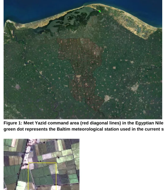
Figure 1: Meet Yazid command area (red diagonal lines) in the Egyptian Nile Delta. The green dot represents the Baltim meteorological station used in the current study.
Figure 2: A high-resolution 5 m IKONOS image (of a different year) with the selected 240 m coarse-resolution image (yellow box) superimposed, to illustrate how the 240 m pixel size relates to individual field sizes.
2.2 Wheat and berseem yields
The main winter crops in the focal area are wheat and berseem (Trifolium alexandrium, L.) and the main summer crops are maize, cotton, and rice (Egypt Farm-level Irrigation Modernization
!
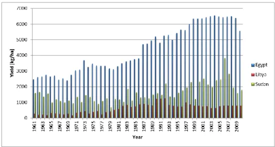
Project (EFIMP), 2010). Minor winter crops are pulses, barley and sugar beet. Since the focus of this study is only on the winter season, with berseem and wheat being the main crops, it is interesting to know the yields of these crops in Egypt, especially in the focal area. Figure 3 represents the annual wheat yield (fresh yield) in Egypt, Libya, and Sudan for the period 1961-2010 (FAOSTAT). It is clear that wheat yields in Egypt are significantly higher than in its neighboring countries Libya and Sudan. It is also clear that wheat yields in Egypt have almost tripled over the last 40 years. Several studies give an indication of the potential wheat yield in Egypt. According to Liu et al. (2007) the potential wheat yield in Egypt is 6617 kg/ha, while Abaza (2009) mentions a potential wheat yield of 8571 kg/ha. The potential wheat yield in the focal area is different from the country’s potential wheat yield, and will be determined later on in this report (Section 4.1). Berseem, also known as Egyptian clover, is grown either over 3 months with 2 cuts as a soil improver, usually preceding cotton, or grown over 6-7 months, either with 4-5 cuts as a fodder crop or grazed by gathered cattle. Because of this, the actual berseem yields in Egypt are unknown. However, berseem is also grown in other countries where the berseem yields have been recorded. For the current study, it is assumed that
potential berseem yields in Egypt are equal to the potential berseem yields in Afghanistan (80 to 100 tons per ha (Oushy, 2008)).
Figure 3: Wheat yield in Egypt, Libya, and Sudan for the period 1961-2010 (source: FAOSTAT).
2.3 Overview
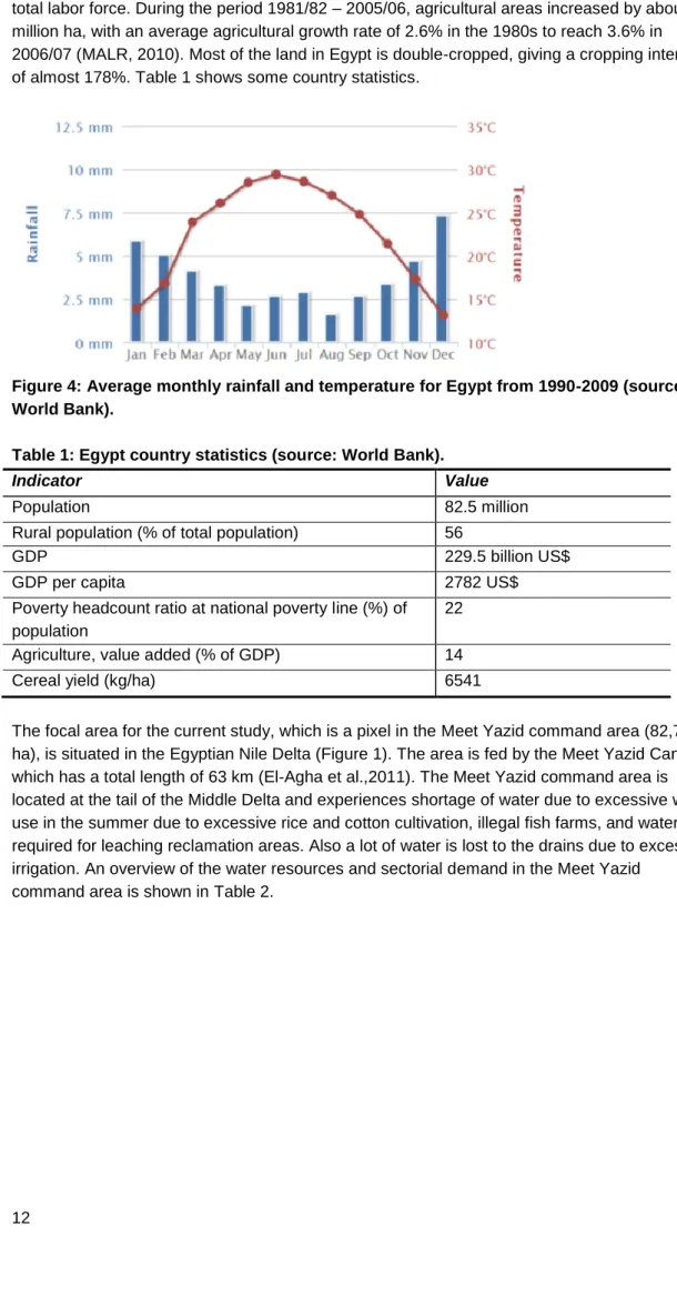
Agriculture in Egypt is mainly irrigated, and is almost entirely dependent on irrigation from the River Nile. This is related to the fact that there is no significant rainfall, except in a narrow strip along the Mediterranean Cost. Egypt has a moderate climate (Figure 4) with a low average monthly rainfall that varies between 1.5 and 7.5 mm/month. Based on these small amounts of rainfall, it is clear that irrigated agriculture plays a crucial role for a wealthy crop production. Temperatures vary between 13°C in December to 30°C in June.
total labor force. During the period 1981/82 – 2005/06, agricultural areas increased by about 1.0 million ha, with an average agricultural growth rate of 2.6% in the 1980s to reach 3.6% in 2006/07 (MALR, 2010). Most of the land in Egypt is double-cropped, giving a cropping intensity of almost 178%. Table 1 shows some country statistics.
Figure 4: Average monthly rainfall and temperature for Egypt from 1990-2009 (source: World Bank).
Table 1: Egypt country statistics (source: World Bank).
Indicator Value
Population 82.5 million
Rural population (% of total population) 56
GDP 229.5 billion US$
GDP per capita 2782 US$
Poverty headcount ratio at national poverty line (%) of population
22
Agriculture, value added (% of GDP) 14
Cereal yield (kg/ha) 6541
The focal area for the current study, which is a pixel in the Meet Yazid command area (82,740 ha), is situated in the Egyptian Nile Delta (Figure 1). The area is fed by the Meet Yazid Canal, which has a total length of 63 km (El-Agha et al.,2011). The Meet Yazid command area is located at the tail of the Middle Delta and experiences shortage of water due to excessive water use in the summer due to excessive rice and cotton cultivation, illegal fish farms, and water required for leaching reclamation areas. Also a lot of water is lost to the drains due to excessive irrigation. An overview of the water resources and sectorial demand in the Meet Yazid
Table 2: Water resources and sectorial demand in the Meet Yazid command area (source: MALR, 2010).
Resources Volume (MCM/year)
Surface water 1669
Ground water 6
Re-use (official) 110
Other Un-official re-use from drains at the tail ends
of canals
Sectorial demand and use Volume (MCM/year)
Irrigation 1820
Municipal 44
Industry negligible
The soils in the middle Delta of the Nile are generally derived from the Nile alluvium. The top soil is predominately clay (Bastiaanssen et al., 1996) with some layers of lighter silt soil. The top soil has high capacity for water holding and low water intake rate. Generally these soils are deep and poorly drained and structured. Natural drainage conditions are very poor over most of the command area (MALR, 2010). A drain spacing of 20 m and a drain depth that varies between 0.6 and 1.5 m, are quite common in the focal area (Amer and de Ridder (1989); Bastiaanssen et al. (1996)).
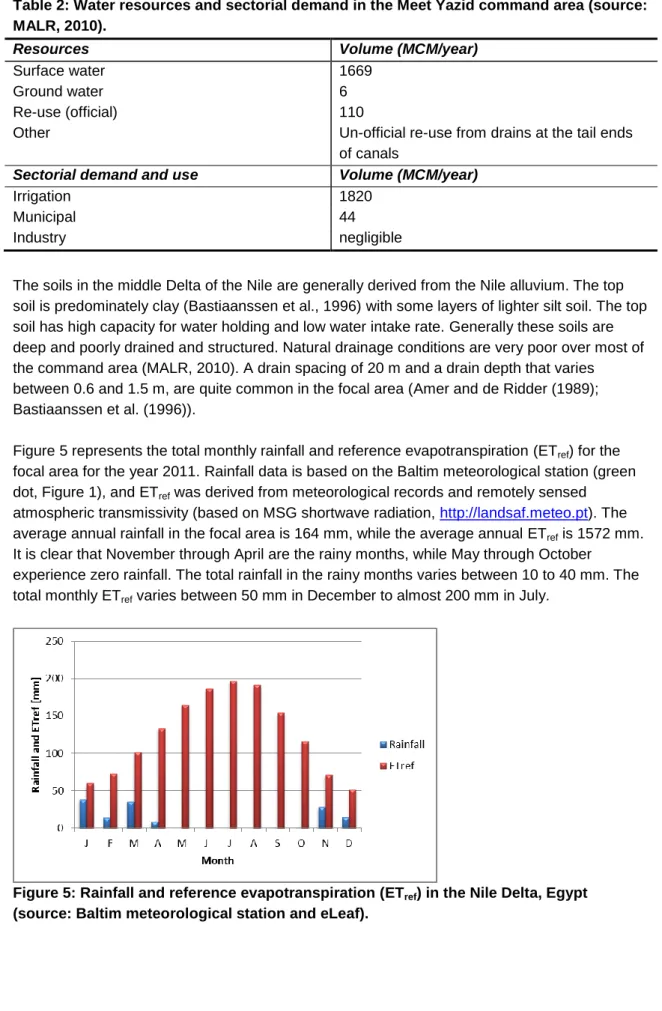
Figure 5 represents the total monthly rainfall and reference evapotranspiration (ETref) for the
focal area for the year 2011. Rainfall data is based on the Baltim meteorological station (green dot, Figure 1), and ETref was derived from meteorological records and remotely sensed
atmospheric transmissivity (based on MSG shortwave radiation, http://landsaf.meteo.pt). The average annual rainfall in the focal area is 164 mm, while the average annual ETref is 1572 mm.
It is clear that November through April are the rainy months, while May through October experience zero rainfall. The total rainfall in the rainy months varies between 10 to 40 mm. The total monthly ETref varies between 50 mm in December to almost 200 mm in July.
Figure 5: Rainfall and reference evapotranspiration (ETref) in the Nile Delta, Egypt (source: Baltim meteorological station and eLeaf).
3
Data and methodology
3.1 Field data
3.1.1 Cropping patterns
As part of the farm-level irrigation modernization project, GeoMAP4 conducted fieldwork in the Meet Yazid command area. One of the main components of this fieldwork was to identify the crop types on the sampled fields. The combination of remote sensing and fieldwork crop classifications has led to crop distributions within the coarse-resolution pixel (Figure 2); 131 pixels wheat, 86 pixels berseem, 31 pixels built-up area, and 8 pixels being other crop types. The growing season starts on the 1st of November, and ends the 14th of May. The simulation period for the current study focuses on the growing season 1-Nov-2011 through 14-May-2012. The individual high-resolution pixels (15 m) that where identified are shown in Figure 6.
Figure 6: High-resolution pixel classification within the selected coarse-resolution pixel.
3.1.2 Yields
A second important component of the fieldwork was to require information regarding the actual yields at the end of the growing season. Farmers explained that the average actual yield for wheat is on average 5357 kg/ha in the Meet Yazid command area. As was mentioned in Section 2.2, and confirmed during fieldwork, berseem is cut several times during the growing
4 http://www.geomap.com.eg/
season and is used as fodder crop or grazed by gathered cattle. Therefore, the berseem yields have not been registered for the study area. For the current study, it is assumed that potential berseem yields in Egypt are equal to the potential berseem yields in Afghanistan (80 to 100 tons per ha (Oushy, 2008)).
3.2 Remote sensing and SEBAL
3.2.1 Available and selected satellite data
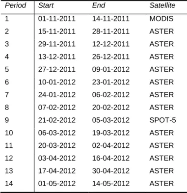
An overview of the bi-weekly availability of satellite imagery is shown in Table 3. It is clear that ASTER imagery is available for nearly all periods, except for the first and ninth bi-weekly period. To create a high-resolution image for the first period, the MODIS image has been resampled using a correction factor. This correction factor is calculated as the ratio between the average of the high-resolution image, averaged over period 2-14, and the average of the coarse-resolution image (MODISr), averaged over the same period. Subsequently the high-resolution image for
each pixel for the first period is calculated by multiplying the correction factor for that pixel with the MODIS image of that period. For period nine a SPOT-5 (Haij et al., 2009; Immerzeel et al., 2005) image (10 m resolution) was available, which was resampled to the 15 m resolution. An overview of some ASTER imagery of the focal area is shown in Figure 7.
Table 3: Overview of available satellite imagery per period (bi-weekly).
Period Start End Satellite
1 01-11-2011 14-11-2011 MODIS 2 15-11-2011 28-11-2011 ASTER 3 29-11-2011 12-12-2011 ASTER 4 13-12-2011 26-12-2011 ASTER 5 27-12-2011 09-01-2012 ASTER 6 10-01-2012 23-01-2012 ASTER 7 24-01-2012 06-02-2012 ASTER 8 07-02-2012 20-02-2012 ASTER 9 21-02-2012 05-03-2012 SPOT-5 10 06-03-2012 19-03-2012 ASTER 11 20-03-2012 02-04-2012 ASTER 12 03-04-2012 16-04-2012 ASTER 13 17-04-2012 30-04-2012 ASTER 14 01-05-2012 14-05-2012 ASTER
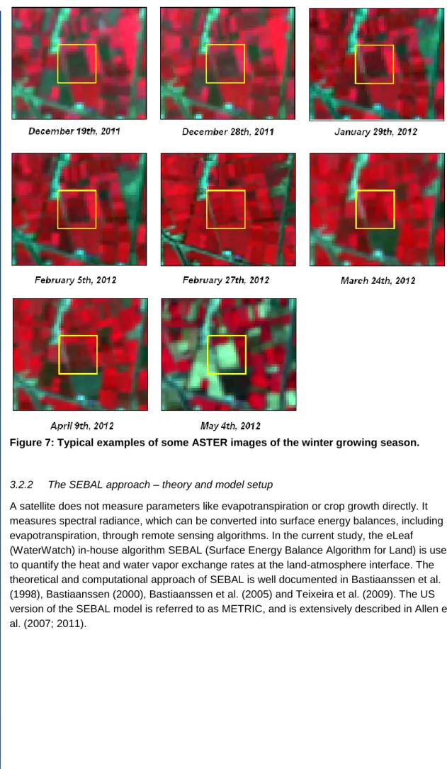
Figure 7: Typical examples of some ASTER images of the winter growing season.
3.2.2 The SEBAL approach – theory and model setup
A satellite does not measure parameters like evapotranspiration or crop growth directly. It measures spectral radiance, which can be converted into surface energy balances, including evapotranspiration, through remote sensing algorithms. In the current study, the eLeaf
(WaterWatch) in-house algorithm SEBAL (Surface Energy Balance Algorithm for Land) is used to quantify the heat and water vapor exchange rates at the land-atmosphere interface. The theoretical and computational approach of SEBAL is well documented in Bastiaanssen et al. (1998), Bastiaanssen (2000), Bastiaanssen et al. (2005) and Teixeira et al. (2009). The US version of the SEBAL model is referred to as METRIC, and is extensively described in Allen et al. (2007; 2011).
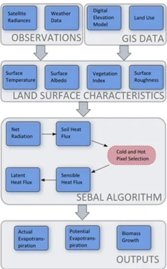
Figure 8: Schematic view of the SEBAL algorithm.
Figure 8 provides a schematic overview of the SEBAL algorithm. In this study, the SEBAL model is applied biweekly during the period from November 1st 2011 until May 14, 2012, defined as the main winter cropping season in the Nile Delta. Satellite radiances are converted first into land surface characteristics such as surface albedo, Leaf Area Index (LAI), vegetation index and surface temperature. No data on soil type or hydrological conditions are required to apply SEBAL. Inputs additional to satellite images consist of a digital elevation model (obtained from the NASA SRTM mission) and a basic satellite-derived land use map, discriminating between water, vegetated areas, bare soil and built-up area. Also, the SEBAL model requires routine weather data parameters: wind speed, relative humidity, and air temperature. These are acquired from the meteorological station Baltim (green dot Figure 1).
The primary basis for the SEBAL model is the surface energy balance. The instantaneous actual evapotranspiration (ETact) flux is calculated for each cell of the remote sensing image as a “residual” of the surface energy budget equation:
differences in energy balance behavior of the different surfaces to get a first estimate on the surface energy balance for all pixels.
In Equation (1), the soil heat flux (G) and sensible heat flux (H) are subtracted from the net radiation flux at the surface (Rn) to compute the "residual" energy available for
evapotranspiration (λE). Soil heat flux is empirically calculated as a G/Rn fraction using
vegetation indices, surface temperature, and surface albedo. Sensible heat flux is computed using wind speed observations, estimated surface roughness, and surface to air temperature differences that are obtained through a sophisticated self-calibration between dry (λE≈0) and wet (H≈0) pixels. SEBAL uses an iterative process to correct for atmospheric instability caused by buoyancy effects of surface heating.
The λE time integration in SEBAL is split into three steps. The first step is to compute the instantaneous evaporative fraction. The second step is the conversion from the instantaneous evaporative fraction into 24 hour values by making the evaporative fraction variable according to advection conditions. The evaporative fraction EF is:
EF = λE/ (Rn - G) (-) (2)
The 24 hour latent heat flux can be determined as:
λE24 = ψ EF Rn,24 (W/m 2
) (3)
where ψ is a correction term that accounts for the EF variability. For simplicity, the 24 hour value of G is ignored in Equation (3). The second step is the conversion from a daily latent heat flux into monthly values, which has been achieved by application of the Penman - Monteith equation:
λEPM = (sa Rn,24 + ρacp Δe/ra) / (sa + γ (1 + rs/ra)) (W/m 2
) (4)
where sa (mbar/K) is the slope of the saturated vapor pressure curve, ρacp (J/m 3
K) is the air heat capacity, Δe (mbar) is the vapor pressure deficit, γ (mbar/K) is the psychrometric constant and ra (s/m) is the aerodynamic resistance. The parameters sa, Δe and ra are controlled by
meteorological conditions, and Rn and rs by the hydrological conditions.
The SEBAL computations can only be executed for cloudless days. The result of λE24 from Eq. (3) has been explored to convert the Penman - Monteith equation (Eq. 4) and to quantify rs
inversely using λE24= λEPM. The spatial distribution of rs so achieved, will consequently be used
to compute λE24 by means of Equation (4) for all days without satellite images available
(Bastiaanssen and Bandara, 2001). The total ETact for a given period can be derived from the
longer term average λE flux by correcting for the latent heat of vaporization and the density of water. The resulting actual evapotranspiration (ETact) is the sum of evaporation from bare soil or
open water bodies and the transpiration of crops. The ETact from the SEBAL algorithm is crop
type independent, which makes SEBAL applicable in areas where a detailed description of the land use is lacking.
Biomass production is calculated according to the principles of the ecological production model of Monteith (1972). This model is based on total Active Photosynthetically Absorbed Radiation (APAR) and a light use efficiency (ε) that converts the radiation absorbed into a dry matter production value. Sunshine duration is used to compute global radiation on a day-to-day basis.
The interception of this radiation by biological active canopies is derived from the vegetation index. The light use efficiency is approximated as a maximum value for c3 crops (2.5 gr MJ
-1
) and a reduction factor depending on the opening of the stomata (Bastiaanssen and Ali, 2003). The opening of the stomata is inversely proportional to the canopy resistance rs. Hence, the
energy balance is also used for the derivation of crop yield.
3.2.3 Harvest Index and biomass
The Harvest Index (HI) is defined as:
Y = BM * HI (5)
where BM is the biomass (dry matter), Y the yield (dry matter), and HI the harvest index. To get the fresh yield, a correction with the moisture content is required:
Y = BM * HI / (1-θ)
with θ being the moisture content. The average (with SEBAL determined) biomass for wheat in the Meet Yazid focal area is 13867 kg/ha. Based on this number and the average actual fresh wheat yield of 5357 kg/ha (Section 3.1.2) in the area, the calculated HI (moisture corrected) for wheat is 0.39. This value is used later on (Section 4.1), in combination with the biomass from a representative wheat pixel, to calculate the actual wheat yield for that pixel. Subsequently, the actual yield can be used to calculate the potential wheat yield using the FAO33 method (see Section 3.3.2.3 (Doorenbos and Kassam, 1979)). As mentioned before, for berseem no yields have been registered and therefore for berseem a potential yield of 90,000 kg/ha is assumed.
3.3 Simulation modeling
3.3.1 SWAP description
The Soil-Water-Atmosphere-Plant (SWAP) model (van Dam, 2000; Kroes et al., 2008) was selected as the tool for performing the simulation modeling component of the project. SWAP is developed at Wageningen University and is the successor of the agro-hydrological model SWATR(E) (Feddes et al., 1978). SWAP was selected as “the” modeling tool for the current study, because it simulates the soil moisture content in the soil profile, which is a major process in the determination of the actual transpiration and reduction of photosynthesis as a result of drought stress (de Wit and van Diepen, 2007). Other reasons for the selection of SWAP are:
Since the scope of the current project is to evaluate the added value of high-resolution remote sensing (e.g. LAI, KC) above coarse-high-resolution remote sensing, it is a huge advantage that the user can assign remotely sensed LAIs and crop factors (KCs) to SWAP, instead of simulating these variables like more complex crop growth models do (e.g. WOFOST (Boogaard et al., 1998; Supit et al., 1994;
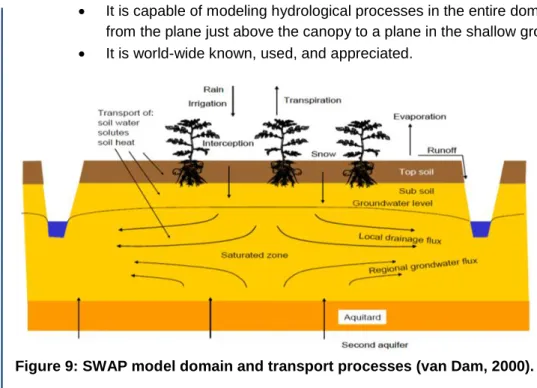
It is capable of modeling hydrological processes in the entire domain (Figure 9) from the plane just above the canopy to a plane in the shallow groundwater;
It is world-wide known, used, and appreciated.
Figure 9: SWAP model domain and transport processes (van Dam, 2000).
SWAP simulates transport of water, solutes and energy in the vadose zone in interaction with vegetation development. In this zone water and solute transport processes are predominantly vertical, and therefore SWAP is a one-dimensional, vertically directed model. The water transport module in SWAP is based on the Richards’ equation, which is a combination of Darcy’s law and the continuity equation.
Figure 10 shows the schematization of the SWAP model. The vertical flow of water through a 1-D column with defined soil layer characteristics is simulated, with the upper boundary condition consisting of meteorological data (including rain and evapotranspiration) and irrigation inputs, corrected by an interception component dependent on the Leaf Area Index (LAI). The bottom boundary is controlled by soil water pressure head, flux, or the relation between head and flux. Actual transpiration depends on the moisture and salinity conditions in the root zone, weighted by the root density. Actual evaporation depends on the capacity of the soil matrix to transport water to the soil surface. This capacity is determined by the soil water retention and hydraulic functions. Surface runoff is calculated when the height of water ponding on the soil surface exceeds a critical depth. SWAP also simulates drainage, which is incorporated as a sink term in the numerical solution of the Richards’ equation. For field-scale applications, often the drainage equations of Hooghoudt (Hooghoudt, 1940) and Ernst (Ernst, 1956) are used.
Figure 10: Schematization of the SWAP model (van Dam, 2000).
Irrigation inputs to the model can be prescribed at fixed times, scheduled according to different criteria, or by using a combination of both. In this way, SWAP provides the option of simulating irrigation conditions under a rotational schedule, where water availability is fixed at certain days; being the traditional situation in the Egyptian Nile Delta, and a continuous flow system where the timing of irrigation application will be determined by the farmers’ interpretation of crop water stress. Crop water stress and automatic water supply can be expressed as the fraction of actual and potential transpiration (Tact/Tpot). If Tact/Tpot, denoted as Tstress hereafter, drops below a
certain value (like e.g. 0.90), SWAP triggers a certain amount of irrigation water supply.
3.3.2 Data and model schematization
The SWAP model input consists of files for main input, meteorological data, crop growth, and drainage. To evaluate the added value of high-resolution remote sensing above coarse-resolution remote sensing in crop yield forecasting, the following data is required:
Meteorology (rain and reference evapotranspiration)
Soil hydraulic parameters
Crop information
Drainage information
Initial soil water condition
Bottom boundary condition
Irrigation scheduling
The current study uses data obtained from a mix of field observations, field surveys, and remote sensing interpretation. Not all the required data, however, was locally available or could be retrieved from remote sensing. Fortunately, many studies have already been performed in this study area (Bastiaanssen et al., 1996; Amer and de Ridder, 1989). Therefore, data from other studies, which were conducted in the proximity of the study areas, are used in the current study
3.3.2.1 Meteorology – upper model boundary
Rainfall plus irrigation, minus the sum of transpiration, evaporation and interception determines the amount of infiltration in the soil and groundwater fluxes. In general, the sums of rainfall plus irrigation and transpiration plus evaporation plus interception are large compared to their difference, which equals infiltration. This means that relative errors in these sums will increase relative errors in infiltration and groundwater fluxes. Therefore, it is very important to have accurate data on rainfall and evapotranspiration. These meteorological fluxes form, together with irrigation, the upper model boundary.
The meteorological station nearest to the focal area is Baltim (green dot Figure 1). Besides rainfall, the reference evapotranspiration (ETref) is of major importance. The ETref, in
combination with the crop factor (Kc), determines the potential transpiration. In SWAP there is
an option to let the model calculate the ETref using the Penman-Monteith equation (Monteith,
1965), or to provide SWAP with ETref values. In the current study, the ETref was derived from
meteorological records and remotely sensed atmospheric transmissivity (based on MSG shortwave radiation, http://landsaf.meteo.pt). This provides us with the most accurate ETref
estimates available for the study areas, and therefore a good basis for deriving the potential evapotranspiration (ETpot).
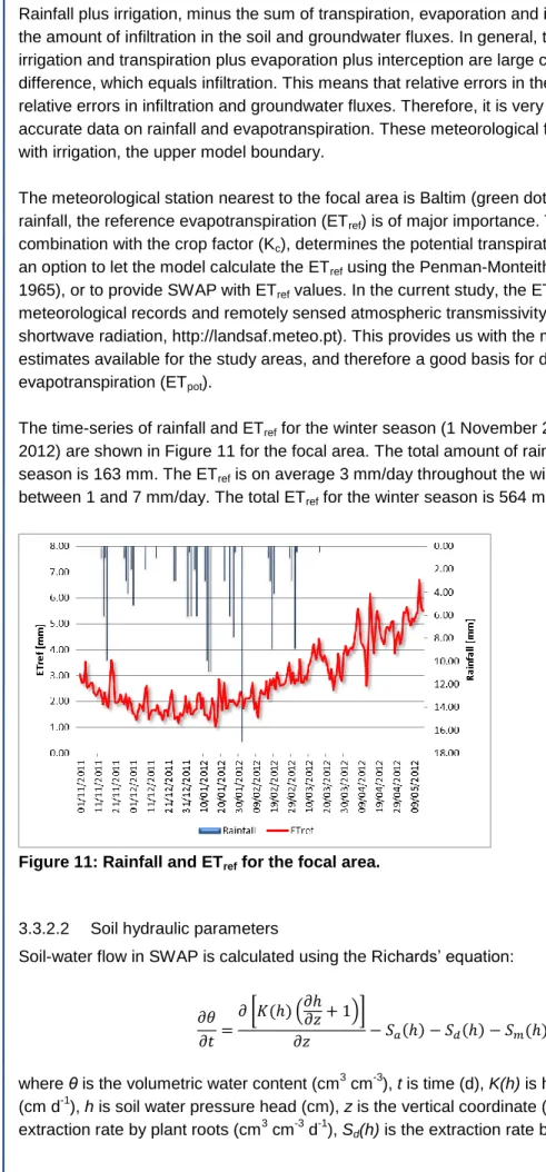
The time-series of rainfall and ETref for the winter season (1 November 2011 through 14 May
2012) are shown in Figure 11 for the focal area. The total amount of rainfall during the winter season is 163 mm. The ETref is on average 3 mm/day throughout the winter season, and varies
between 1 and 7 mm/day. The total ETref for the winter season is 564 mm.
Figure 11: Rainfall and ETref for the focal area.
3.3.2.2 Soil hydraulic parameters
Soil-water flow in SWAP is calculated using the Richards’ equation:
[ ( )]
where θ is the volumetric water content (cm3 cm-3), t is time (d), K(h) is hydraulic conductivity (cm d-1), h is soil water pressure head (cm), z is the vertical coordinate (cm), Sa(h) is soil water
saturated zone (d-1) and Sm(h) is the exchange rate with macro pores (d
-1
). SWAP solves this equation numerically, using known relations between θ, h, and K. These relations are
expressed in the water retention curve and the unsaturated hydraulic conductivity curve. These curves are often derived from laboratory measurements. If these curves are known, then the Mualem-Van Genuchten (Van Genuchten, 1980) function can be used to fit a curve to the measured curves. The resulting soil hydraulic parameters are then subsequently used to parameterize the soil layers in the SWAP model.
Parameterization
Bastiaanssen et al. (1996) performed a study towards the transportability and inter-comparison of crop-water-environment-models in the Nile Delta in Egypt. They derived a pF-curve (Figure 12) and unsaturated hydraulic conductivity curve (Figure 13) for the Zenkalon area in the Nile Delta. These soils were taken as representative for the focal area, because they belong to the same black to brown clay loam soil types as the soils in the study area (Amer and de Ridder, 1989). Using the Mualem-Van Genuchten function (Van Genuchten, 1980) the curves were fitted, and are shown as simulated curves in Figure 12 and Figure 13. The soil parameters corresponding with these curves are shown in Table 4. These soil parameters will be used as initial parameter values for the calibration, and will be optimized during the calibration process (Section 3.3.3).
Figure 12: Observed pF curve for Zenkalon derived according to laboratory
measurements and model calibration (Bastiaanssen et al., 1996) and simulated pF curve using Mualem-Van Genuchten function (van Genuchten, 1980).
Figure 13: Observed unsaturated hydraulic conductivity curve for Zenkalon derived according to estimations, laboratory measurements, and model calibration
(Bastiaanssen et al., 1996) and simulated unsaturated hydraulic conductivity curve using Mualem (1976).
Table 4: Derived SWAP soil-physical parameters. Θres cm3/cm3 Θsat cm3/cm3 α 1/cm n - Ksat cm/d λ - 0.05 0.50 0.1139 1.4068 22.09 2.0213 Schematization
The soil profile in SWAP is schematized by the vertical discretization of the soil profile. In addition to the natural soil layers with different hydraulic functions, the thickness and number of calculation compartments should be defined. For the correct simulation of infiltration and
evaporation fluxes near the soil surface, the compartment thickness near the soil surface should be ≤ 1 cm (Van Dam, 2000). Deeper in the soil profile, where the soil water flow is less dynamic, the compartment thickness may increase to 10 cm (Van Dam, 2000). For numerical stability, the soil profile was discretized as shown in Table 5.
Table 5: Schematization of the SWAP soil profile. Soil sub
layer
Depth
[cm below surf.]
Height soil compartment [cm] Number of soil compartments 1 0 - 10 1.0 10 2 10 - 30 5.0 4 3 30 – 60 5.0 6 4 60 - 200 10.0 14
3.3.2.3 Crops and irrigation application
SWAP contains three crop growth routines: a simple module, a detailed module (WOFOST, World Food STudies), and a detailed module for grass (re)growth. Since the objective of this study is to evaluate the added value of high-resolution above coarse-resolution satellite imagery in crop yield forecasting, we should minimize the number of variables that are not related to the high- and coarse-resolution images, and that can affect crop yield forecasting. Examples of such variables are nitrogen and phosphorus applications, pests, diseases, and pollutants.
These variables, among others (e.g. CO2), are also not available for the focal area; meaning
that the model outcome would be based on many uncertain variables. Then the outcome of the current study would be more a reflection of the uncertainty in detailed crop growth model input parameters, instead of the added value of high- versus coarse-resolution imagery in crop yield forecasting. Therefore, we have chosen to use the simple crop growth module in SW AP. Within this simple module, the user can specify as function of the development stage (Figure 15):
The LAI or soil cover fraction;
The crop factor (Kc) or crop height;
The rooting depth;
Stress criterion (Tstress) to trigger irrigation applications; Irrigation depth;
Figure 14: Reduction coefficient for root water uptake, αw as function of soil water pressure head h and potential transpiration rate Tp (Feddes et al., 1978).
To calculate irrigation timing and actual transpiration SWAP uses the root water uptake reduction function (Figure 14, Feddes et al. 1978). The simple crop growth model does not calculate the potential or actual yield. However, the user can define yield response factors (Doorenbos and Kassam, 1979; Smith, 1992) for various growing stages as a function of the development stage. Subsequently, for each growing stage k the actual yield Ya,k (kg/ha) relative
to the potential yield Yp,k (kg/ha) during this growing stage is calculated by:
(
)
where Ky,k(-) is the yield response factor of growing stage k, ETp,k (cm) and ETa,k (cm) are the
Figure 15: Typical partitioning of assimilated dry matter among leaves, stem, roots and storage organs as function of development stage (Van Dam, 2000).
Parameterization
As mentioned before, the user has to specify the LAI, Kc, rooting depth, Tstress, and irrigation
depth as function of the crop’s development stage. For each ASTER pixel, being either berseem or wheat, the two weekly LAI and Kc were obtained from the remote sensing image, and were subsequently specified in the SWAP crop files. The same is done for the coarse-resolution pixel, being only one LAI and Kc time-series, representing a mixture of wheat, berseem, build-up area, and another crop.
The rooting depths of berseem and wheat have not been measured in the focal area. However, some literature values exist (Allen et al., 1998) on these depths and these were optimized during the calibration process.
The irrigation frequencies and depths in the focal area are not accurately known. Therefore, both the irrigation frequency and irrigation depth will be determined during the calibration process.
For the calculation of the relative yield, SWAP uses the yield response factor Ky. The yield
response factors for wheat and berseem have been obtained from Allen et al. (1998), and are 1.05 for wheat and 1.1 for berseem.
SWAP allows for the calculation of solute transport and crop stress as a result of too high salinity levels. Since solute simulation and a reduction in crop growth due to too high salinity levels is not the scope of the current study, this option in SWAP has been turned off. Stress in crop growth in the current study can therefore only occur as a result of water shortage.
3.3.2.4 Drainage
The amount of drainage water is a function of crop type and irrigation management,
meteorological conditions, and soil characteristics. For SWAP, several drainage characteristics are needed, such as the drain spacing, drain depth, wet perimeter, and entrance resistance.
Schematization and parameterization
Unfortunately, no field-specific drainage information is available for the focal area. However, there is enough information available regarding the “classic” drainage systems in Egypt.
According to Amer and De Ridder (1989) and Bastiaanssen et al. (1996), drainage depths in Egypt can vary between 1.5 m and 0.6 m. For the current study we applied a drainage depth of 1.0 m, which is within the classical ranges often found in Egypt. A commonly used drain spacing in Egypt is 20 m (Amer and de Ridder (1989); Bastiaanssen et al. (1996)). According to the final report of technical support for on-farm improvements in W-10 (Mohamed, 2008), this drain spacing is also commonly used in the focal area. Therefore, a drain spacing of 20 m is used for all simulations. For the drainage resistance a value of 60 days is assumed.
3.3.2.5 Initial condition
Within SWAP three options exist to define the initial soil moisture condition: 1. Pressure head as function of depth is input;
2. Pressure head of each compartment is in hydrostatic equilibrium with initial groundwater level;
3. Read final pressure heads from output of previous SWAP simulation.
Actual groundwater levels have not been measured in the focal area. However, groundwater levels in the Nile Delta in Egypt are quite shallow, and are often within 1 m from the surface (Bastiaanssen et al., 1996; Amer and de Ridder, 1989). For the current study we have assumed an initial groundwater level of -80 cm. The initial soil moisture conditions for the current study were subsequently determined using option 1, where both the initial groundwater level and the pressure head as function of the soil depth were further optimized during the calibration.
3.3.2.6 Bottom boundary condition
SWAP has several options for defining the bottom boundary condition. These options describe the relation between saturated shallow soil layers with the deep groundwater. According to Amer and de Ridder (1989), the study area is located in a zone with an upward seepage rate of 0.2 mm/d. SWAP offers the option to define a prescribed bottom flux (qbot), which is positive
upwards and negative downwards. This option has been implemented in the current study; a prescribed bottom flux of 0.2 mm/d (upward).
3.3.3 SWAP calibration and validation
3.3.3.1 Representative pixel selection
SWAP needs to be calibrated and validated in order to give reliable crop yield forecasts. Since the fraction of the actual evapotranspiration (ETact) over the potential evapotranspiration (ETpot)
indicates the relative crop yield, SWAP has been calibrated such that the simulated ETact
matches the measured ETact from SEBAL, on a two-weekly basis. For the current study, SWAP
has been calibrated separately for a representative wheat pixel and a representative berseem pixel. Preceding the calibration, first a representative wheat and berseem pixel had to be selected. This selection is based on the distribution of ETact for wheat and berseem. First a
3.3.3.2 Calibration with PEST
The calibration of SWAP is done using the Model-Independent Parameter Estimation software PEST5. PEST is used as calibration tool for the current study because it uses a powerful, yet robust, estimation technique that has been tested on a wide range of problem types (e.g. Christensen and Doherty, 2008; Dausman et al., 2010; Doherty, 2003; Doherty and Hunt, 2009; Doherty and Hunt, 2010). During the calibration process, PEST will adjust the model
parameters until the fit between the model output and field observations is optimized in the weighted least squares sense. More details regarding PEST can be found in Doherty (2004).
Calibration was initiated for wheat with 20 adjustable parameters. After the first calibration attempt, it seemed that many parameters did not have a significant effect on the calibration result. Therefore, many parameters were set as fixed during the second calibration attempt, meaning that they cannot be adjusted by PEST. The first calibration attempt resulted in an initial groundwater level of -83 cm. This value was fixed in the second calibration attempt, where an additional parameter was introduced to determine the pressure head (Hini) at a depth of -10 cm. During the second calibration attempt a total of 12 parameters were optimized as shown in Table 6.
Since berseem grows in the same area as wheat, the initial soil moisture conditions and soil hydraulic parameters were taken from the calibrated wheat parameters. Therefore, for berseem the soil hydraulic parameters and initial soil moisture parameter were not used during the calibration, as shown in Table 7. The calibration results of both wheat and berseem are shown in Section 3.3.3.3.
Table 6: Calibration parameters and resulting calibrated values for wheat.
Parameter Description Final parameter value
ORES Residual water content [cm3/cm3] 0.035 ALFA Shape parameter alfa of main drying curve [1/cm] 0.15
NPAR Shape parameter n [-] 1.165
KSAT Saturated vertical hydraulic conductivity [cm/d] 28.70 COFRED Soil evaporation coefficient of Black [cm/d1/2] 0.10 Hini Initial pressure head at -10 cm [cm] -200.95 CFBS Coefficient to derive ETpot from ETref [-] 0.526 TREL5 Daily stress criterion at development stage 1.5 [-] 0.98 TREL6 Daily stress criterion at development stage 2.0 [-] 0.98 FID1 Fixed irrigation depth at development stage 0.0 [mm] 23.8 R3 Rooting depth at development stage 0.5 [cm] 24.7 R4 Rooting depth at development stages 1.0 till 2.0 [cm] 70.6
5 http://www.pesthomepage.org/
Figure 16: Boxplot of SEBAL actual evapotranspiration (ETa) for all high-resolution wheat pixels during the growing season (period 1-14). The colored lines represent a selection of individual wheat pixels. Periods are defined as two-weekly periods.
Figure 17: Boxplot of SEBAL actual evapotranspiration (ETa) for all high-resolution berseem pixels during the growing season (period 1-14). The colored lines represent a selection of individual berseem pixels. Periods are defined as two-weekly periods. Table 7: Calibration parameters and resulting calibrated values for berseem.
Parameter Description Final parameter value
COFRED Soil evaporation coefficient of Black [cm/d1/2] 0.10 TREL1 Daily stress criterion at development stage 0.0 [-] 0.50 TREL2 Daily stress criterion at development stage 0.25 [-] 0.50 TREL3 Daily stress criterion at development stage 0.5 [-] 0.50 TREL4 Daily stress criterion at development stage 1.0 [-] 0.50 TREL5 Daily stress criterion at development stage 1.5 [-] 0.97 TREL6 Daily stress criterion at development stage 2.0 [-] 0.50 FID1 Fixed irrigation depth at development stage 0.0 [mm] 10.0 FID2 Fixed irrigation depth at development stage 0.5 [mm] 10.0 FID3 Fixed irrigation depth at development stage 1.0 [mm] 8.9 FID4 Fixed irrigation depth at development stage 1.5 [mm] 17.5 FID5 Fixed irrigation depth at development stage 2.0 [mm] 1.0 R1 Rooting depth at development stage 0.0 [cm] 0.0 R2 Rooting depth at development stage 0.25 [cm] 0.0 R3 Rooting depth at development stage 0.5 [cm] 20.0 R4 Rooting depth at development stages 1.0 till 2.0 [cm] 63.3
3.3.3.3 Results Wheat
Wheat was calibrated for the representative wheat pixel with ID 87. Figure 18 shows for each period (2-weekly) the observed versus the uncalibrated and calibrated ETa. The ETa was simulated too high for the uncalibrated wheat pixel during the first three periods. During the last three periods the ETa was simulated too low for the uncalibrated wheat pixel. It is clear that the calibrated ETa fits the observed ETa better. A scatter-plot of the observed vs. the uncalibrated and calibrated wheat ETa is shown in Figure 19. It is clear that the calibrated pixel performs better (R2 = 0.90) than the uncalibrated pixel (R2 = 0.36).
Figure 18: Actual observed and simulated evapotranspiration for wheat. Results are shown for each 14-day period for both the uncalibrated and the calibrated wheat pixel with ID 87.
21. It is clear that the validated ETa matches the observed ETa almost perfectly (R2 = 0.94). The validation result for wheat is slightly better than the calibration result for wheat, which may be due to some noise.
Figure 20: Actual observed and simulated evapotranspiration for wheat. Results are shown for each 14-day period for the validated wheat pixel with ID 170.
Figure 21: Scatter-plot of observed versus simulated actual evapotranspiration for wheat. Results are shown for the validated wheat pixel with ID 170.
Berseem
Berseem was calibrated for the representative berseem pixel with ID 22. Figure 22 shows for each period (2-weekly) the observed versus the uncalibrated and calibrated ETa for berseem. Also for berseem, SWAP simulates the ETa too high for the uncalibrated pixel during the first three periods. The ETa is also simulated too high for the uncalibrated pixel during the last period. It can be concluded that calibration has led to promising results; for nearly every period the simulated ETa is a good fit to the observed ETa. A scatter-plot of the observed vs. the uncalibrated and calibrated berseem ETa is shown in Figure 23. It is clear that the calibrated pixel performs better (R2 = 0.89) than the uncalibrated pixel (R2 = 0.57).
The calibrated berseem pixel parameters were also tested (validated) for another berseem pixel. This validation was done for berseem pixel 63. Results of the validated berseem pixel are shown in Figure 24 and Figure 25. With a correlation-coefficient of 0.80 it can be concluded that berseem is validated satisfactory. Only during the second and last period the ETa is
underestimated.
Figure 22: Actual observed and simulated evapotranspiration for berseem. Results are shown for each 14-day period for both the uncalibrated and the calibrated berseem pixel with ID 22.
Figure 23: Scatter-plot of observed versus simulated actual evapotranspiration for berseem pixel with ID 22. Both the uncalibrated and calibrated results are shown.
Figure 24: Actual observed and simulated evapotranspiration for berseem. Results are shown for each 14-day period for the validated berseem pixel with ID 63.
Figure 25: Scatter-plot of observed versus simulated actual evapotranspiration for berseem. Results are shown for the validated berseem pixel with ID 63.
Table 8: Calibration and validation statistics for wheat and berseem.
A water balance gives an overview of all the incoming and outgoing fluxes of water. The water balance for both the calibrated wheat and calibrated berseem pixel is shown in Table 9. It is clear that more irrigation is applied to wheat (119 mm) than for berseem (80 mm). This is related to the fact that berseem is more “drought” resistant than wheat. Rootwater uptake reduction for wheat already starts at a pressure head of -500 cm, while a reduction in rootwater uptake for berseem starts at a pressure head of -1500 cm. Due to the potential higher
Pixel R2 [-] RMSE [mm/14 days]
Wheat uncalibrated (pixel 87) 0.36 12.8
Wheat calibrated (pixel 87) 0.9 6.5
Wheat validated (pixel 170) 0.94 4.5
Berseem uncalibrated (pixel 22) 0.57 10.8
Berseem calibrated (pixel 22) 0.89 4.7
transpiration for berseem, the actual transpiration for berseem is higher than for wheat. Both drainage and soil evaporation are relatively small for both wheat and berseem.
Table 9: Water balance for the calibrated wheat (left table) and berseem (right table) pixel.
3.4 Crop yield forecasting
To evaluate the added value of high-resolution above coarse-resolution remote sensing images in crop yield forecasting, it is required to have a reference data set which represents the “real” crop yield situation in the field. In other words, this data set is the observed data as would have been measured during that growing season. To create this reference data set, the SWAP model has been run for all fourteen periods, using high-resolution ASTER imagery as input for all these periods. This run will be referred to as the reference run hereafter.
Crop growth models are commonly used to predict crop growth during the last two months of the growing season. Since the current growing season covers the period 1-Nov-2011 through 14-May-2012, the entire period consists of fourteen two-weekly periods. Therefore, the last four two-weekly periods are used as the crop yield forecasting period, being the last two months of the growing season. For the coarse-resolution crop yield simulation we have used the MODISr
LAIs and KCs for the first ten two-weekly periods, whereas for the high-resolution crop yield simulation we have used the ASTER LAIs and KCs for the first ten two-weekly periods. The last four two-weekly periods are the forecasting period (two months). In reality no remote sensing images are available for the forecasting period. To use representative LAIs and KCs during the forecasting period, “standard values” are used for both the high- and coarse-resolution
simulations. The current study uses MODISr imagery as “standard values” for the forecasting
period. The use of satellite imagery in the three defined runs is summarized in Table 10 and illustrated in Figure 26.
Table 10: Summary of the satellite imagery used during the first period and the forecasting period.
Run First period Forecasting period
Reference ASTER ASTER
High-resolution ASTER SV6
Coarse-resolution MODISr SV
6
Wheat water balance In [mm] Out [mm]
Rain 163 -Irrigation 119 -Interception - 10 Transpiration - 224 Evaporation - 39 Runoff - 0 Drainage - 22 Qbot 39 dS 26
Berseem water balance In [mm] Out [mm]
Rain 163 -Irrigation 80 -Interception - 16 Transpiration - 312 Evaporation - 32 Runoff - 0 Drainage - 25 Qbot 39 -dS -103
Figure 26: Illustration of the use of LAIs in the three runs which are compared in the current study. The last four two-weekly periods (2 months) are used as the forecasting period.