New Jersey Institute of Technology
Digital Commons @ NJIT
Theses Theses and Dissertations
Spring 2014
Risk prediction with genomic data
Bharati Jadhav
New Jersey Institute of Technology
Follow this and additional works at:https://digitalcommons.njit.edu/theses
Part of theBioinformatics Commons, and theComputer Sciences Commons
This Thesis is brought to you for free and open access by the Theses and Dissertations at Digital Commons @ NJIT. It has been accepted for inclusion in Theses by an authorized administrator of Digital Commons @ NJIT. For more information, please [email protected].
Recommended Citation
Jadhav, Bharati, "Risk prediction with genomic data" (2014).Theses. 199.
Copyright Warning & Restrictions
The copyright law of the United States (Title 17, United
States Code) governs the making of photocopies or other
reproductions of copyrighted material.
Under certain conditions specified in the law, libraries and
archives are authorized to furnish a photocopy or other
reproduction. One of these specified conditions is that the
photocopy or reproduction is not to be “used for any
purpose other than private study, scholarship, or research.”
If a, user makes a request for, or later uses, a photocopy or
reproduction for purposes in excess of “fair use” that user
may be liable for copyright infringement,
This institution reserves the right to refuse to accept a
copying order if, in its judgment, fulfillment of the order
would involve violation of copyright law.
Please Note: The author retains the copyright while the
New Jersey Institute of Technology reserves the right to
distribute this thesis or dissertation
Printing note: If you do not wish to print this page, then select
“Pages from: first page # to: last page #” on the print dialog screen
The Van Houten library has removed some of the
personal information and all signatures from the
approval page and biographical sketches of theses
and dissertations in order to protect the identity of
NJIT graduates and faculty.
ABSTRACT
RISK PREDICTION WITH GENOMIC DATA by
Bharati Jadhav
Genome wide association study (GWAS) is widely used with various machine learning
algorithms to predict disease risk. This thesis investigates this widely used approach of
GWAS using Single Nucleotide Polymorphism (SNP) genotype data and a novel approach
of disease risk prediction with whole exome sequencing data, namely Whole Exome Wide
Association Study (WEWAS). It further applies a discriminating machine learning
algorithm, namely a Support Vector Machine (SVM) with different Kernel functions. For
this study, only SNPs generated using genotyping technology, which focuses more on
common variants, are used initially for disease prediction. Later, the whole exome data
generated using Next Generation Sequencing (NSG) technology is used in the prediction.
Another distinction between traditional GWAS and the new approach, WEWAS, presented
in this thesis is the use of insertions and deletions in the genomic sequence (INDEL)
together with SNPs as a feature for prediction. A substantial improvement in the prediction
accuracy is achieved using the latter approach. The success of the approach of using NSG
data shows that it contains valuable information which the SNP genotyping method is
unable to capture.
RISK PREDICTION WITH GENOMIC DATA
by Bharati Jadhav
A Thesis
Submitted to the Faculty of New Jersey Institute of Technology
in Partial Fulfillment of the Requirements for the Degree of Master of Science in Bioinformatics
Department of Computer Science May 2014
APPROVAL PAGE
RISK PREDICTION WITH GENOMIC DATA
Bharati Jadhav
Dr. Usman Roshan, Thesis Advisor Date Associate Professor of Computer Science, NJIT
Dr. Jason T Wang, Committee Member Date Professor of Computer Science, NJIT
Dr. Zhi Wei, Committee Member Date Associate Professor of Computer Science, NJIT
BIOGRAPHICAL SKETCH
Author: Bharati Jadhav
Degree: Master of Science Date: May 2014
Undergraduate and Graduate Education: • Master of Science in Bioinformatics,
New Jersey Institute of Technology, Newark, NJ, 2014 • Master of Science in Computers,
University of Pune, Pune, India, 2000 • Bachelor of Science in Computers,
University of Pune, Pune, India, 1998 Major: Bioinformatics
v
ACKNOWLEDGMENT
I wish to thank you my advisor, Dr. Usman Roshan, for supervising for his continuous
help, support and encouragement to shape my interest and ideas. His guidance helped me
in all stages of my research.
I also like to thank Dr. Zhi Wei and Dr. Jason T. Wang for serving on my masters
thesis committee. Additionally, the knowledge I gained through their courses has
tremendously helped me for this thesis.
In the end, I would like to express my gratitude to my husband, Chetan, for
believing in me and supporting me through hard time. I am also grateful to my two
wonderful children, Sid and Smruti, for their understanding and patience. Without them I
vi
TABLE OF CONTENTS
Chapter Page
1. INTRODUCTION………. 1
2. GENOME-WIDE ASSOCIATION STUDIES………. 3
2.1.What is Genome-wide Association Study?……… 3
2.2.Evolution of Genome-wide Association Study……….. 4
3. METHODS AND DATA……….. 6
3.1.Data Sets………. 6
3.1.1. GWAS Data………. 6
3.1.2. WEWAS Data………. 7
3.2.Analysis Procedure……… 8
3.2.1. Quality Control of GWAS Data………. 10
3.2.2. Quality Control of WEWAS Data……….. 11
3.3.Feature Selection………... 12
3.4.Multiple Comparison problem and Bonferroni correction……… 13
3.5.Feature Encoding……….. 14
3.5.1. GWAS Data……… 14
3.5.2. WEWAS Data……… 14
3.6.Machine Learning: Classification with SVM………... 15
3.6.1. SVM Kernel functions………... 16 3.6.2. Cross validation………. 16 4. RESULTS……… 18 4.1.GWAS Data……….. 18 4.1.1. GIC Data……… 19 4.1.2. BC Data………. 21 4.2.WEWAS Data……….. 22 5. CONCLUSION………... 26
vii
LIST OF TABLES
Table Page
3.1 Description of Datasets Used In This Study………. 6
3.2 Description of Datasets Platform Used In This Study……….. 7
4.1 Whole Data Association……… 18
4.2 Train and Test Dataset Details of BC and GIC before QC……….. 19
4.3 Train and Test Dataset Details of BC and GIC after QC………. 19
viii
LIST OF FIGURES
Table Page
3.1 Experimental design of GWAS………. 9
3.2 Experimental design of WEWAS………. 10
3.3 QC steps of WES data……….. 12
4.1 QQ plot of GIC data………. 20
4.2 Prediction accuracy of GIC……….. 21
4.3 QQ plot of BC data………... 22
4.4 Prediction accuracy of BC……… 23
1 CHAPTER 1 INTRODUCTION
This research investigates the use of machine learning algorithm for diseases prediction
using case-control association analysis. This study tested SNP genotype data, as used in
traditional GWAS, as well as NSG data with this machine learning approach to determine
the prediction accuracy. In the first part of this study, prediction is done using GWAS data.
This study uses three sets of features for prediction. First set of features includes only
significant SNPs found using univariate method, second set includes the pair of SNPs
interacting with each other significantly and third set comprises the SNPs from previous
two sets, univariate as well as interacting SNPs. This study is further extends to the novel
approach, WEWAS, of using NGS data with machine learning algorithm.
In genetic case-control studies, the frequency of allele is compared between the
group of affected individuals and the group of healthy individuals. If there is a significant
difference in the allele frequency between these two groups then that allele is consider to
be a causal variant, and it may increase the disease risk. In the machine learning approach,
these variants are further used as a feature vector with classification algorithm to predict
the disease risk. For prediction of risk, one of the state of art machine learning algorithms,
Support Vector Machine (SVM)[1], is used. SVM has already proven its success in many
computational biology applications [2].
This thesis is organized as follows: Chapter 2 gives introduction of GWAS, and its
evolution to current state. Chapter 3 discusses the data and methods in depth used for this
2
differences in the Quality Control measures and feature encoding required for SVM due to
the nature of data. The methodology section in this chapter also covers the feature selection
and ranking using chi-square statistical test, multiplicity control, SVM and its different
Kernel functions used for classification. Chapter 4 discusses the analysis of results of
predictions accuracy obtained with different sets of feature and different Kernel functions
3 CHAPTER 2
GENOME-WIDE ASSOCIATION STUDIES
2.1What is Genome-wide Association Study?
GWAS is a method to study many common genetic variants in different individuals to see
if they are associated with particular disease. There exists many kinds of genetic variants
in human genome. This includes insertion, deletions, inversion, replication of segment of
DNA within a chromosome, or segment of DNA moved to a different location in the same
or different chromosome. GWAS seeks to identify one simple and common type of variant,
Single Nucleotide Polymorphism (SNP), which happens when single nucleotide base in
DNA sequence is replaced with a different base. There are an estimated 10 million SNPs
that are commonly occur in human genome [3]. In GWAS, the distribution of SNP is
determined in hundreds or thousands of subjects with and without particular disease. The
researchers can calculate the co-existence of SNP with disease status and can make
statistical estimate regarding the increased risk associated with each SNP. In the era of
2005-2007 many GWAS were published which led to the identification of common genetic
variants associated with several common disease. These studies includes but not limited to
Type 1 and Type 2 diabetics, Crohn’s disease, rheumatoid arthritis, etc.[4].
DNA microarray play a vital role in GWAS which made possible to genotype
hundreds of thousands of SNPs quickly and relatively at low-cost. Many manufactures of
DNA microarray now offers to genotype more than million SNPs. These huge number of
genotyped data is assessed to find the association of SNPs with disease. Even though
GWAS using SNP markers has widely used for discovery of genetic risk factors in human
4
that are common in population. Also, the genetic variants that are low in frequency and
have small effects on traits are difficult to detect using GWAS [5]. Additionally, genetic
variants that are of high frequency with strong effects are very unusual for common
diseases. Lastly, population stratification, linkage disequilibrium, and DNA Pooling can
bias the results. These short comings of GWAS, can be addressed using NGS data which
not only focuses on common variants but also includes the rare variants.
2.2 Evolution of Genome-wide Association Study
NGS technology allows researcher to address diverse range of biological problems at
detailed levels never than before, because of its high throughput, scalability, and speed.
NGS provides high flexibility in adjusting the level of resolution required for the
experiment. The custom-made sequencing run allows to zoom into particular region of
genome and produce high resolution data or provide bigger picture of genome with less
resolution. This leads to two broad categories of DNA sequencing using NGS technology:
Whole Genome Sequencing (WGS) and Whole Exome Sequencing (WES). WGS reads
entire DNA of individual. It is possible to reveal all de-novo and low frequency alleles that
contributes to the disease risk with WGS. Despite this fact, WGS is still expensive to
perform on very large sample size. The WES fills the gap between GWAS and WGS. The
WES captures only DNA which code for proteins, exome, also known as coding regions.
The exome comprise around 1-2% of whole genome but many cancer causing variants are
found within this coding regions. This reduces the sequencing need up to 98%. It is faster
5
sequencing, this technique constitutes an interesting approach for the identification of point
mutations and small INDELs with high accuracy.
This flexibility of NGS technology becomes very useful to find rare variants by
having a high resolution to detect the rare variants in the human genome which is hard with
GWAS. The variants which occur at low frequency requires large number of samples to be
sequence and today it is possible to with this technology in a few days. With the advent in
the DNA sequencing technology, now it is possible to perform GWAS using NGS data and
extent these studies to rare variants.
6
CHAPTER 3
METHODS AND DATA
3.1Data Sets
Five different cancer data sets are used in this experiment. All the data sets are available
on The Database of Genotype and Phenotypes (dbGaP) [6]. It is a repository of results from
the studies such as GWAS and medical sequencing. First four datasets from GWAS are
generated using SNP genotyping technology and the last dataset of WEWES is generated
using WES. The Table 3.1 below describes the details of data used in this study.
Table 3.1 Description of Datasets Used In This Study
Dataset No. of Cases No. of Controls dbGaP Study Accession GIC 3523 2100 phs000361.v1.p1 BC 3527 5119 phs000346.v1.p1 RCC 1311 3424 phs000351.v1.p1 PC 1563 2593 phs000206.v3.p2 CLL 169 169 phs000435.v2.p1
Source: Database of Genotypes and Phenotypes (dbGaP). Bethesda (MD): National Center for Biotechnology Information, National Library of Medicine.
3.1.1 GWAS Data
The first dataset of Bladder Cancer (BC) consist of collection of 8646 individuals and
approximately one million SNPs. This dataset consist of five subsets of data genotyped on
different platforms. The Gastro-Intestinal Cancer (GIC) dataset contains data from two
7
approximately 600,000 SNPS. The third dataset of Pancreatic Cancer (PC) contains 5,078
individuals and approximately 630,000 SNPs. The last SNP genotype data, Renal Cell
Carcinoma (RCC) consists of 4735 individuals and approximately 700,000 SNPs.
Additional details are given in the Table 3.2 below.
Table 3.2 Description of Datasets Platform Used in this Study
Dataset No. of
Cases
No. of Controls
Platform
GIC 3523 2100 Illumina Human 660 W BC 3527 5119 Illumina Human 610 HumanHap 250 HumanHap 300 HumanHap 550 Illumina Human 1M RCC 1311 3424 Illumina Human 610 Illumina Human 660 W Illumina HumanHap 550 PC 1563 2593 Illumina Human 610 HumanHap 550
CLL 169 169 Illumina Whole Exome Sequencing
Source: Database of Genotypes and Phenotypes (dbGaP). Bethesda (MD): National Center for Biotechnology Information, National Library of Medicine.
3.1.2 WEWAS Data
The whole exome sequencing data used in later part of the thesis is whole exome sequences
of 169 chronic lymphocytic leukemia patients. For each of 169 patients, data is sequenced
for tumor and matched healthy cell. The whole exome sequencing libraries were
8
exomic regions were captured using Agilent Sureselect All Human exome kit by Broad
Institute and comprises 76 bp pair-end-reads [7]. The data was sequenced to obtain
approximately mean coverage of 140X. Additional details are given in the Table 3.2 above.
3.2 Analysis Procedure
The main goal of case control association study is to test the difference between allelic
frequency in cases and controls to find the variants that are associated with disease. As this
study usually includes large number of samples to detect the small effect and studies
hundreds of thousands of markers, even small artifact in allelic frequency can leads to false
signals [8]. The overall quality control play important role in downstream analysis and if
not properly done can result in false positive results. Therefore, before starting actual data
analysis it is necessary to apply appropriate filters to achieve accuracy in downstream
analysis and avoid bias in the study. The same experimental design is applied to SNP
genotype data and whole exome data for association study and classification, however, the
quality control steps are quite distinct due to the nature of data as each one used different
technology. The quality filtering steps are described in the Sections 3.2.1 and 3.2.2 below.
Next step after filtering data is to find the significant variants and rank them
according to their significance from most significant to least significant. This is achieved
by chi-square test and described in the Section 3.3 below.
In both types of data called variants were used for further statistical analysis which
includes ranking variants, multiplicity control, and classification. Feature vectors were
formed by encoding SNPs and INDELs, and classification was done to predict accuracy of
9
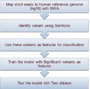
The traditional association study considers SNPs which are in Linkage
Disequilibrium (LD) and do not consider the interaction between the SNP which are
located far apart from each other in large genome. To investigate the inclusion of
interacting SNPs in risk prediction, a new approach of using interacting SNPs pairs along
with SNPs found by univariate method was used with GWAS GIC and BC dataset. The
pair of interacting SNPs were found using SIXPAC program [9]. The prediction accuracy
with the set of interacting SNPs alone as well as combining with set of significant SNPs
found using univarite method was tested with different Kernel functions. The overview of
experimental design of GWAS is given in Figure 3.1 below.
Figure 3.1 Experimental design of GWAS.
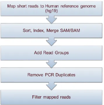
The WEWES data involved many data manipulation steps before quality control and
variant calling. The first was to map the raw reads to the human reference genome Hg19
10
perform on the mapped reads such as sort, index, merge the alignment map files using
Samtools [10] (version 0.1.18) and add read group information using PICARD (version
1.8). The sketch of experimental design of WEWAS is given in the Figure 3.2 below.
Rigorous quality control steps were performed on WEWES data at different stages before
calling variants as described in the Section 3.3.2 below.
Figure 3.2 Experimental design of WEWAS.
3.2.1 Quality Control of GWAS Data
Even though genotyping technology and allele calling algorithms are continue to improve
and make sure that only reliable markers and samples are included, the sex or familial
relationship can cause sample identity problems such as, sample relatedness which lead to
Type I and Type II errors. To avoid such problems rigorous quality control measures were
taken on SNP genotype data. The quality control was performed on each of four genotype
11
removing duplicated or related individual to follow the basic feature of standard,
population based case-control studies that all samples should be unrelated. Otherwise, it
introduces bias to studies because of over representation of genotypes within families. The
samples with missing phenotype status were also removed. The chromosomes X, Y, and
MT are haploid and counted only once. Not all genotype calling algorithm automatically
set heterozygous haploid genotype missing [12]. Therefore, the genotypes for these
chromosomes were set to missing. Next, the SNPs with missing rate 1% more were
excluded from the analysis. Finally, the SNPs which deviates from HWE principle were
remove with cutoff 5%, because these SNPs can be indication of genotyping or genotype
calling error.
3.2.2 Quality Control of WEWAS Data
The NGS technology generate huge number of sequencing data. Checking the quality of
generated data is the first step in the variant calling pipeline. There are two main steps
involved to extract variants from raw sequencing data. First step is to map the reads to the
reference genome HG19 and then identify variant sites and determine the genotypes for
those variants. But the variant identification step suffers from high error rate due to the low
quality read, especially at the tail which prevent reads from being properly mapped. Also,
the PCR artifact create bias in the results. There are some quality control steps which can
be applied to the sequencing data before mapping, such as checking quality of reads, trim
low quality read tails if needed and other steps can be applied after mapping the reads to
the reference genome. For example, remove low quality reads, unmapped read and remove
PCR duplicates. The pre-alignment quality control steps such as check raw read quality
12
applied to few samples on experimental basis, but did not find any significant improvement
in mapping. Additionally, given the huge number of samples to process, these two steps
were skipped and used only the raw reads for mapping to the reference genome. After
mapping step, unmapped reads were removed. Furthermore, reads with MAPQ, which is
score lower than 15 were also removed using Samtools. Duplicates in the reads arises from
the artifacts during PCR amplification and sequencing. These duplicate reads, sampled
from the DNA molecule, map to the same position on the reference genome many times.
This uneven representation of that DNA molecule introduces bias in identification of
variant. Therefore, the duplicate reads were removed using PICARD tool. The QC steps
are depicted in the Figure 3.3 below.
13
3.3Feature Selection
In machine learning feature selection play important role when it comes to hundreds and
thousands of features. Feature selection is a process of selecting subset of relevant features
from the set of irrelevant or redundant features and use them in the model construction.
The redundant features do not provide additional information and the irrelevant features do
not contribute any information which create unnecessary noise in the data. Feature
selection helps to resolve this issue. Many studies have demonstrated that the use of feature
selection approach with high dimensional data such as DNA sequencing data generated by
high throughput sequencing technology, can improve the prediction accuracy with machine
learning algorithms [2]. Feature selection methods in machine learning are broadly divided
into filter, wrapper and embedded methods. Filter methods for genetic feature selection are
the most common in GWAS due to the simplicity of their implementation and low
computational complexity. The filter methods calculate a univariate test statistic separately
for each genetic feature, and the features are then ranked based on the observed statistic
values. The highest ranked features form the final set of selected features, on which a
predictive model can be trained. This thesis focuses on the finding the risk related variants
and not finding the interaction among the variants, therefore, the chi-square test was used
for feature ranking. The Chi-square univariate test is a standard method of feature selection
in GWAS [14]. This method investigates each SNP independently and tests if there is
difference in the frequency of alleles observed in the cases vs controls. If this difference is
significant, then the SNP is associated with disease. In this research study, the chi-square
method was applied on both data types to find contributing features. The p-value of this
14
variants. Then the variants were ranked in the order of decreasing p-value. The highly
ranked variants were used as a features with machine learning algorithm, SVM, to predict
the accuracy of classification.
3.4Multiple Comparison Problem and Bonferroni Correction
The multiple comparison problem arises when number of comparisons increases in the
statistical testing such as Chi-square. The standard p-value cutoff used is 5%. This means
that there are 5% chances of having false positive. The GWAS scans hundreds of thousands
of variants to identify candidate variants that are associated with disease. With such high
number of tests the error rate multiples and generates huge number of false positive variants
which are not significant at all. This leads to the Type I error, which occurs when there is
no real association between variants and disease but results into false positive. GWAS are
more prone to Type I error because of multiple testing. The standard threshold of p-value
cutoff used with most of the statistical method to reject the null hypothesis is not enough
with GWAS data, because even with 0.05, it produces hundreds and thousands of false
positive variants. This makes interpretation of association study difficult.
This multiple comparison problem in GWAS can be solved by adjusting p-value.
The Bonferroni correction is one of the approaches used for controlling Type I error [15].
It is an adjustment made to the p-value to control when multiple statistical tests are
performed. It is achieved by dividing the critical p-value by the number of comparison
being made. This correction reduces the chances of introducing false positives (Type I
error). 0.05 p-value . Adjusted No of SNPs (3.1)
15
3.5Feature Encoding
The machine learning algorithm requires features in numeric format, hence all the variants
were encoded from text to numeric format.
3.5.1 GWAS Data
Each individual can have 0, 1 or 2 copies of minor allele and contribution of each copy of
minor allele make a numeric value of phenotype. The basic allelic test for association, done
using PLINK, counts the frequency of minor allele in cases and controls and perform a
chi-square test with 1-degree of freedom.
3.5.2 WEWAS Data
In whole exome sequencing data SNPs were encoded in 0, 1 or 2 based on if it is
homozygous reference, heterozygous, or homozygous alternate. The INDELs were
encoded as a difference between the length of allele string in the reference and alternate,
where the negative number indicate deletion in the sequence and positive number indicate
insertion in the given sequence. If INDEL is not present in some sample it is encoded as 0.
3.6Machine Learning: Classification with SVM
Many Machine learning methods are extensively use in the field of Bioinformatics, such
as genomics, microarrays, proteomics to name a few to extract knowledge from the huge
amount of data [16]. One of the application of machine learning is a classification which
is widely used in GWAS to measure and analyze genetic variation in DNA sequence across
the human genome to identify disease causing variants. There exists many classifier to
16
performing supervised learning algorithm because of its high accuracy, capacity to handle
high dimensional data [17] and hence it is widely for GWAS applications [2]. Additionally,
it has the ability to generate nonlinear decision boundaries to classify non-linearly
separated data by constructing linear boundaries in the transformed version using Kernel
function of the features, which are genomic variants in this case.
The significant variants were encoded in the numerical format required for
SVM-light (Version 6.02) [18]. The SVM training algorithm was applied to the set of significant
variants and prediction was done by discriminating between cases and controls. This risk
prediction model was build using the 90% of total data to form training dataset and
remaining 10% was used as test dataset. The grid search on SVM parameter C and
prediction error of model was assessed using cross validation technique.
3.6.1 SVM Kernel Functions
This study also evaluated the performance of different Kernel functions of SVM such as
Linear, Polynomial Degree 2 and Radial Basis Function (RBF). A Kernel method is an
algorithm that depends on the data only through dot products. The Kernel function
computes a dot products in some high dimensional feature space. This leads to generate
nonlinear decision boundaries and allows to apply a classifier to the data that have no fix
dimensional vector space representation which is applicable to the genomic data [17]. As
machine learning is data dependent, the best way to find the Kernel suitable for particular
data is to try different Kernels. Based on this fact, the motive behind testing different
Kernel functions with each datasets used in the study, was to see if the prediction accuracy
increases if data is transformed in another feature space. Initially, Linear Kernel was
17
were applied on each dataset. With GWAS data all the Kernels were used with default
settings. Whereas, with WEWAS data the value of SVM penalty parameter C, which
controls misclassification, was found by grid search and all the other parameters were used
with the default setting.
3.6.2 Cross Validation
The method of cross validation leads to good estimate of algorithm performance [19]. The
performance measure from the k-fold cross validation can be used to tune the algorithm.
In this method the dataset is randomly split into k exclusive subsets of approximately same
size. These data sets are further used to train and test the algorithm. The cross validation
accuracy estimate is the number of correct classification divided by the number of
randomly split data sets. The grid search on penalty parameter C was also performed using
cross validation with the values ranging from 0.01 to 100 and the best cross validation
accuracy was picked for all the Kernel functions. In this thesis the methodology explain
18 CHAPTER 4
RESULTS
4.1 GWAS Data
For this thesis four cancer GWAS dataset were studied to predict the disease risk. To test
the usability of each dataset, whole data association analysis was performed in the initial
stage of the study. The details of the initial whole data association are shown in the Table
4.1. This analysis helped to provide good idea about each of the BC, GIC, RCC, and PC
datasets and based on it the PC and RCC datasets were eliminated from the further study.
The RCC data contained many noisy signals which were more than found in the original
study [20]. On the other hand, PC data showed only two signals which were not enough
for prediction. Therefore, first 100 SNPs from the set of ranked SNPs of PC were used for
prediction but resulted into only 48% of accuracy. The other two datasets, BC and GIC
were used further in the downstream analysis. Each dataset was divided into random split
of 90/10. The quality control steps were applied on the 90% of training dataset and was
used to build a model which further used with 10% data to predict the accuracy. Table 4.2
shows the QC details of BC and GIC before performing QC and Table 4.3 shows the details
after QC.
Table 4.1 Whole Data Association
Dataset No. of Sample No. of SNPs No. of Signals GIC 5,623 491,777 7
BC 8,646 200,315 5 PC 5,078 425,510 2 RCC 4,909 481,932 247
19
Table 4.2 Train and Test Dataset Details Of BC and GIC before QC
Dataset No. of Sample No. of Cases No. of Controls No. of SNPs
GIC Train 5,052 3,188 1,864 592,839
GIC Test 571 325 236 592,839
BC Train 7,792 3,171 4,621 1,116,724
BC Test 854 356 498 1,116,724
Table 4.3 Train and Test Dataset Details of BC and GIC after QC
Dataset No. of SNPs before Cleaning No. of SNPs after cleaning
GIC Train 592,839 491,884
BC Train 1,116,724 200,840
4.1.1 GIC Data
The GIC dataset performed well with this investigation. The association analysis reported
total seven SNPs (rs3781264, rs753724, rs11187842, rs3765524, rs2274223, rs12263737,
and rs3740360) which passed the Bonferroni correction threshold. Out of these 7 SNPs
five SNPs (rs3781264, rs753724, rs11187842, rs3765524, and rs2274223) are in
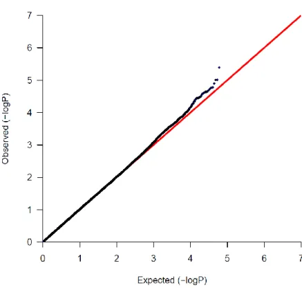
concordance with the SNPs found in the original study [21]. The Q-Q plot of GIC shows
the distribution of association (X-axis) across the set of significant SNPs compared to the
observed values (Y-axis). The deviation from X=Y line implies a consistent difference
between cases and controls across the genome. The plot in the Figure 4.1 shows that a line
of observed frequency matches the line of expected frequency until the little deviation at
20
with disease. The blue dot in the Figure 4.1 shows the true disease related variants in the
GIC data.
These significant SNPs were used as features with SVM Linear, Polynomial, and
RBF Kernel for classification. In the Figure 4.2, it can be seen that there is approximately
1.5% variation in prediction accuracy among the feature set formed by Chi-square, pairs
of interacting SNPs and combination both with Linear, Polynomial and RBF Kernel
methods. All the combination gives approximately 58% accuracy. Among these nine
combinations, Linear and Polynomial Degree 2 Kernel work similar with the three types
of feature sets and their performance is better than RBF Kernel.
21
Figure 4.2 Prediction accuracy of GIC.
4.1.2 BC Data
The BC data comprised of five subsets of data and each one was genotyped on different
platform ranging from Illumina HumanHap250Sv1.0 to ILLUMINA_Human_1M. After
merging all these subsets, there were only 200,840 SNPs available for analysis. A total 5
SNPS were found as a significant which passed the Bonferroni correction cutoff.
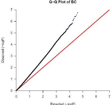
The QQ plot in Figure 4.3 shows a line of observed frequency deviating from the
line of expected frequency and at the tail it shows the small number significant SNPs. The
blue dot in the figure shows the true disease related variants in the BC data. The deviation
of observed frequency from expected frequency can result due to population stratification
[22]. The samples for BC are collected from European decedents from USA and Spain
[23]. The Q-Q plot of BC data shows the population stratification present in this data
collected from heterogeneous population. On the contrary, the GIC data is collected from
58.67 58.67 58.84 58.67 58.67 57.27 58.67 58.67 57.09
LINEAR POLYNOMIAL RADIAL BASIS
% A cc u rac y
22
specific region in China which is much more homogeneous [24]. It is evident from the
Q-Q plot of GIC data that there is no population stratification and the SNPs are truly
associated with disease. The differences between these two plot shows the biases induced
in the GWAS data as it relies on common variants.
Figure 4.3 QQ plot of BC data.
The following Figure 4.4 shows 1% variation in prediction accuracy among the
feature set formed by Chi-square, pairs of interacting SNPs and combination both with
Linear, Polynomial and RBF Kernel methods. All combinations have prediction accuracy
around 58%. Among these nine combinations, Linear Kernel with the pair of interacting
23
Figure 4.4 Prediction accuracy of BC.
4.2 WEWAS Data
The Section 3.2.2 describes in details the method used to obtain feature vectors from raw
exome sequences. In the case of whole exome data the features are counts of SNPs and
INDELs. The collection of variants from exome dataset is referred as feature vectors.
Table 4.4 CLL Variant Details
CLL WEWAS Data Total No. of Variants 335 Samples
(180 cases, 155 controls) 680814
Train Dataset 278
Test Dataset 57
The processed exome sequence data with 155 controls and 180 cases yielded around
680814 variants. This data was divided in training and testing dataset by randomly
58.08 57.96 58.31 58.43 58.08 57.85 58.2 57.61 57.73
LINEAR POLYNOMIAL RADIAL BASIS
% A cc u rac y
24
selecting 90% of total cases and 90% of total controls for training dataset and remaining
10% data was used for testing. The details about variant can be found in the Table 4.4. The
Bonferroni cutoff was applied on the ranked variants which provided ten significant
variants consisting nine SNPs and one INDEL. Top 100 variants were used for
classification using SVM. The Linear and Ploynomial Kernel gave same accuracy of 89%,
while the RBF Kernel performed worse with accuracy of 50%.
Figure 4.5 Prediction accuracy of CLL.
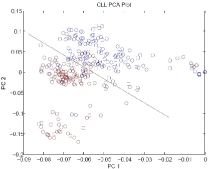
The linear separation between the two classes of data was tested using the PCA plot
as shown in the Figure 4.6 below. The PC 1 and PC 2 are the first and second principal
component respectively. The red circles representing controls and blue circles representing
cases shows clear separation in the PCA plot.
89 89
50
LINEAR POLYNOMIAL RADIAL BASIS
% A cc u rac y Chi-Sq
25
26 CHAPTER 5 CONCLUSION
This investigation shows that the risk prediction using SVM can be equally or potentially
more effective with NGS data than with GWAS data.
In the first part of the study, the association analysis of GIC data found seven
significant SNPs. Surprisingly, when these SNPs were used for predicting disease risk, it
showed very low predictive power and resulted into low accuracy around 58%. The
analysis of BC data also resulted in very few signals and low accuracy.
This study extended the risk prediction using single SNPs to the interacting SNPs
in the great hope to get more predictive power. However, this approach when used with
interacting pair of SNPs only as well as combining it with single SNPs did not make any
improvement in the prediction accuracy. The possible reason might be the inflated p-value
of interacting SNPs generated by the software. This problem can be verify by using another
software to find interacting SNPs and use them in the classification.
To overcome the limitations of GWAS, when the same methodology was applied
to CLL WES data, interesting finding were observed. More investigation is underway. But
one of the interesting observation was, significant improvement in the prediction accuracy.
Future work includes to find the contribution of INDELs and uncommon SNPs in the
prediction accuracy.
The performance of Linear, Polynomial and RBF Kernel function were also
assessed with each dataset. With the GIC and BC data, performance of each kernel function
was similar and accuracy was low. It might be possible because of two reasons. First, the
27
highly imbalanced. This imbalance of data might be producing classifier as a majority class
classifier. On the other hand, the Linear and Polynomial Kernels perform well with the
CLL WES data. The RBF kernel performed worst with the CLL WES data. This is expected
28
REFERENCES
1. Joachims T (1998) Text categorization with Support Vector Machines: Learning with many relevant features. In: Nédellec C, Rouveirol C, editors. Machine Learning: ECML-98. Berlin, Heidelberg, Germany:Springer. pp. 137-142.
2. Wei Z, Wang K, Qu H-Q, Zhang H, Bradfield J, et al. (2009) From disease association to risk assessment: an optimistic view from genome-wide association studies on Type 1 diabetes. PLoS Genet 5: e1000678.
3. Norrgard K (2008) Genetic variation and disease: GWAS Nature Education 1(1):87.
4. Burton PR, Clayton DG, Cardon LR, Craddock N, Deloukas P, et al. (2007) Genome-wide association study of 14,000 cases of seven common diseases and 3,000 shared controls. Nature 447: 661-678.
5. McCarthy MI, Abecasis GR, Cardon LR, Goldstein DB, Little J, et al. (2008) Genome-wide association studies for complex traits: consensus, uncertainty and challenges. Nature Reviews Genetics 9: 356-369.
6. Mailman MD (2007/10) The NCBI dbGaP database of genotypes and phenotypes. Nat Genet 39.
7. Wang L, Lawrence MS, Wan Y, Stojanov P, Sougnez C, et al. (2011) SF3B1 and other novel cancer genes in chronic lymphocytic leukemia. New England Journal of Medicine 365: 2497-2506.
8. Laurie CC, Doheny KF, Mirel DB, Pugh EW, Bierut LJ, et al. (2010) Quality control and quality assurance in genotypic data for genome-wide association studies. Genetic Epidemiology 34: 591-602.
9. Prabhu S, Pe'er I (2012) Ultrafast genome-wide scan for SNP–SNP interactions in common complex disease. Genome Research 22: 2230-2240.
10. Li H, Durbin R (2009) Fast and accurate short read alignment with Burrows–Wheeler transform. Bioinformatics 25: 1754-1760.
11. Purcell S, Neale B, Todd-Brown K, Thomas L, Ferreira MA, et al. (2007) PLINK: a tool set for whole-genome association and population-based linkage analyses. The American Journal of Human Genetics 81: 559-575.
12. Anderson CA (2010/09) Data quality control in genetic case-control association studies. Nat Protocols 5.
13. Bolger AM, Lohse M, Usadel B (2014) Trimmomatic: A flexible trimmer for Illumina sequence data. Bioinformatics 170v1.
29
14. Roshan U, Chikkagoudar S, Wei Z, Wang K, Hakonarson H (2011) Ranking causal variants and associated regions in genome-wide association studies by the support vector machine and random forest. Nucleic acids research 39: e62-e62.
15. Duggal P, Gillanders EM, Holmes TN, Bailey-Wilson JE (2008) Establishing an adjusted p-value threshold to control the family-wide type 1 error in genome wide association studies. BMC genomics 9: 516.
16. Larrañaga P, Calvo B, Santana R, Bielza C, Galdiano J, et al. (2006) Machine learning in bioinformatics. Briefings in Bioinformatics 7: 86-112.
17. Ben-Hur A, Weston J (2010) A user’s guide to support vector machines. Data mining techniques for the life sciences: Springer. pp. 223-239.
18. Joachims T (2009) Svm-light support vector machine, 2002. http://svmlight.joachims. org (accessed on April 28, 2014).
19. Dasgupta A, Sun YV, König IR, Bailey‐Wilson JE, Malley JD (2011) Brief review of regression‐based and machine learning methods in genetic epidemiology: the Genetic Analysis Workshop 17 experience. Genetic Epidemiology 35: S5-S11.
20. Purdue MP, Johansson M, Zelenika D, Toro JR, Scelo G, et al. (2011) Genome-wide association study of renal cell carcinoma identifies two susceptibility loci on 2p21 and 11q13. 3. Nature Genetics 43: 60-65.
21. Abnet CC, Freedman ND, Hu N, Wang Z, Yu K, et al. (2010) Genome-wide association studies of gastric adenocarcinoma and esophageal squamous cell carcinoma identify a shared susceptibility locus in PLCE1 at 10q23. Nature Genetics 42: 764.
22. Chen J, Zheng H, Bei J-X, Sun L, Jia W-h, et al. (2009) Genetic structure of the Han Chinese population revealed by genome-wide SNP variation. The American Journal of Human Genetics 85: 775-785.
23. Rothman N, Garcia-Closas M, Chatterjee N, Malats N, Wu X, et al. (2010) A multi-stage genome-wide association study of bladder cancer identifies multiple susceptibility loci. Nature Genetics 42: 978-984.
24. Li W-Q, Hu N, Hyland PL, Gao Y, Wang Z-M, et al. (2013) Genetic variants in DNA repair pathway genes and risk of esophageal squamous cell carcinoma and gastric adenocarcinoma in a Chinese population. Carcinogenesis 34: 1536-1542.