ISSN: 2088-8708, DOI: 10.11591/ijece.v9i3.pp1506-1513 1506
Relevance vector machine based fault classification in
wind energy conversion system
Rekha S. N.1,P. Aruna Jeyanthy2, D. Devaraj3
1Sapthagiri College of Engineering, India
2,3Kalasalingam Academy of Research and Education (KARE), India
Article Info ABSTRACT
Article history: Received May 15, 2018 Revised Dec 9, 2018 Accepted Jan 2, 2019
This Paper is an attempt to develop the multiclass classification in the Benchmark fault model applied on wind energy conversion system using the relevance vector machine (RVM). The RVM could apply a structural risk minimization by introducing a proper kernel for training and testing. The Gaussian Kernel is used for this purpose. The classification of sensor, process and actuators faults are observed and classified in the implementation. Training different fault condition and testing is carried out using the RVM implementation carried out using Matlab on the Wind Energy Conversion System (WECS). The training time becomes important while the training is carried out in a bigger WECS, and the hardware feasibility is prime while the testing is carried out on an online fault detection scenario. Matlab based implementation is carried out on the benchmark model for the fault detection in the WECS. The results are compared with the previously implemented fault detection technique and found to be performing better in terms of training time and hardware feasibility.
Keywords: Fault detection Gaussian kernel
Relevance vector machine System
Wind energy conversion
Copyright © 2019 Institute of Advanced Engineering and Science. All rights reserved.
Corresponding Author: Rekha S. N.,
Sapthagiri College of Engineering, Bangalore, India.
Email: [email protected]
1. INTRODUCTION
The fault detection in the WECS is an important aspect in the working of the wind power generation system, as the faults occurring in the system would increase the maintenance cost. Development of the overall fault detection including the turbine, generator, converter, pitch and the drive train becomes important considering the cost involved in the maintenance of the WECS. The benchmark model wind turbine for fault identification, which includes the sensor, process and actuator fault condition, is developed [1]. A 4.8 MW WECS model is developed in order to observe the faults in the system. SVM based fault detection is carried out in Wind turbines and compared with the ANN for the accuracy, training and tuning times [2]. The linear SVM performed better in comparison with the ANN. The classification using RVM performed better than the SVM while the training time is said to be higher [3]. Wind generator bearing fault are sensed by the sound and vibration in the tower using empirical mode decomposition method [4]. A nine turbine based wind farm challenge to detect the wind turbine faults in the individual turbine are carried out [5]. A state estimation set membership approach based implementation is found in fault detection of benchmark model with noise [6]. A multi-objective optimization framework for large scale wind turbine system is developed using the
H
¥/
H
- observer to detect the sensor and actuator fault [7]. Especially fault detection is a classification between two classes; normal state or fault and for the classification, support vector machine (SVM) is a useful machine learning method [7], [8], [9] and applications to fault detections are reported [10].This paper takes up the implementation from the benchmark model and implement the RVM on the benchmark model for the wind fault identification problem. The overall faults like the sensor, process and
actuator faults are included in order to classify the faults according the measurement from different sensors from the WECS. Further the paper is sectioned as follows, Section-II would talk about the different sections of the WECS where the fault is detected.Section-III talks about the RVM implementation on the wind fault detection.Section-IV infers the results and discussion followed by the conclusion and the references.
1.1. Wind energy conversion system model
The benchmark model developed in [1] is used in the present implementation. It comprises of the wind model, blade and pitch model, drive train model, generator/converter model, controller and parameters. In the wind model the different sequence of wind is stored as a vector
v
w, which would be used for the input to the wind turbine. The Blade and Pitch model comprises of the aerodynamic and the pitch model of the turbine as defined in (1).2
)
(
))
(
).
(
(
)
(
2 3t
v
t
t
C
R
t
q w r
(1)The aerodynamic torque is defined in equation (1) where
r
is the Air density (kg/m3) ,R
is the rotor radius,C
q rotor torque coefficient,l
tip speed ratio,b
blade pitch angle.If the wind turbine has three blades and thus would have three blade pitch angles. Thus the torque equation would be as defined in (2), which is the sum of torques in all the three blades.
.
6
)
(
))
(
).
(
(
)
(
3 1 2 3
i w i q wt
v
t
t
C
R
t
(2)The reason that
b
value varies for each blade introduces little variation in the torque developed by each blade, though the overall behavior of the model is similar to that of the model with similarb
value. The hydraulic pitch system is a closed loop model defined by a second order transfer function which is a piston servo system.2 2 2
2
)
(
)
(
n n n cs
s
s
s
(3)Equation (3) defines the second order transfer function of hydraulic pitch system where
V
is the damping factor, natural frequency defined byw
n. The transfer function is defined for all three-pitch system in similar way. The damping factor is the same for all the three-pitch system if there are no disturbances. Hydraulic power drop and the increase in air pressure is are the parameters that vary when there is a fault occurrence in the pitch system. The parameters for power drop is defined as
n2and
2and that of the air pressure is
n3and
3. The closed loop pitch actuator being the linear system with change in sensor gain affecting it wouldneed mean of two sensor values to be fed to the actuator. Thus the pitch reference would be changed according to the changes sensor values which is indicated as follows.
𝛽𝑟,𝑓,𝑖[𝑛] = 𝛽𝑟,𝑖[𝑛] −
∆𝛽𝑖,𝑚1[𝑛] + ∆𝛽𝑖,𝑚2[𝑛]
2 (4)
Where 𝑖 ∈ {1,2,3} and 𝛽𝑟,𝑓,𝑖[𝑛] is the reference pitch that gets generated after the disturbance. The model of transferring the torque from rotor to the generator is defined as the drive train model. A gear box in the middle to convert the lower speed to the higher speed is represented as a two mass model defined in (5) and (6).
𝐽𝑟𝜔𝑟(𝑡) = 𝜏𝑟(𝑡) − 𝐾̇ 𝑑𝑡𝜃∆(𝑡) − (𝐵𝑑𝑡+ 𝐵𝑟)𝜔𝑟(𝑡) + 𝐵𝑑𝑡
𝑁𝑔
𝐽𝑔𝜔̇𝑔(𝑡) =𝜂𝑑𝑡𝐾𝑑𝑡 𝑁𝑔 𝜃Δ(𝑡) + 𝜂𝑑𝑡𝐵𝑑𝑡 𝑁𝑔 𝑤r(𝑡) − ( 𝜂𝑑𝑡𝐵𝑑𝑡 𝑁𝑔2 + 𝐵𝑔) 𝜔𝑔(𝑡) − 𝜏𝑔(𝑡) (6) 𝜃̇Δ(𝑡) = 𝜔𝑟(𝑡) − 1 𝑁𝑔 𝜔𝑔(𝑡)
Where 𝐽𝑟the moment of inertia of low speed shaft is, 𝐾𝑑𝑡is the torsion stiffness of the drive train, 𝐵𝑑𝑡is the torsion damping coefficient of the drive train, 𝐵𝑔 is the viscous friction of the high speed shaft. 𝑁𝑔 is the gear
ratio, 𝐽𝑔is the moment of inertia of the high speed shaft. 𝜂𝑑𝑡is the efficiency of the drive train. 𝜃Δ(𝑡) is the torsion angle of the drive train. The fault in the drive train is due to variation in the drive train efficiency which would be denoted by 𝜂𝑑𝑡2 instead of 𝜂𝑑𝑡.
The electrical model which comprises of the generator and the converter which works in frequency which is much higher than the benchmark model is defined by the first order transfer function as defined in (7).
𝜏𝑔(𝑠) 𝜏𝑔,𝑟(𝑠)=
𝛼𝑔𝑐
𝑠 + 𝛼𝑔𝑐 (7)
Where 𝛼𝑔𝑐is the generator and converter parameter. The generator power is defined by (8)
𝑃𝑔(𝑡) = 𝜂𝑔𝜔𝑔(𝑡)𝜏𝑔(𝑡) (8)
where 𝜂𝑔is the efficiency of the generator. The control scheme chosen for this implementation simple as the
focus is on the fault detection of WECS. In order to simplify the benchmark model the drive train damper is avoided. There are two modes in which this implementation would work, one is the power optimization mode and the reference power mode. The power optimization mode is when the speed of the wind is greater than the nominal speed. The controller starts when there is less power generated from the wind energy due to wind speed less than the nominal speed. It is denoted as
𝑃𝑔[𝑛] ≥ 𝑃𝑟[𝑛] ⋁ 𝜔𝑔[𝑛] ≥ 𝜔𝑛𝑜𝑚
where 𝜔𝑛𝑜𝑚is the nominal generator speed and the mode changes from this mode 2 to the mode 1 if 𝜔𝑔[𝑛] ≤ 𝜔𝑛𝑜𝑚− 𝜔Δ
where 𝜔Δ is the offset that is subtracted from the nominal speed to avoid the change from mode 1 to mode 2 and vice versa frequently. The conditions of fault and the mode variation along with the model parameters are used as it is from [1].
2. RELEVANCE VECTOR MACHINE BASED IMPLEMENTATION OF FAULT DETECTION
The different fault conditions are trained on the Relevance Vector Machine (RVM) and a multi class RVM structure is developed in order to test the different fault condition of the wind fault that is considered in [1]. The multiple RVM structures are developed as discussed in [11]. The different fault conditions are as given in the Table 1 is introduced for training the RVM and testing it.
Table 1.Different Fault Conditions Trained Using RVM
Fault No. Fault Type Fault Site Symbols 1a Fixed Value Sensor Faults Blade Positions ∆𝛽1,𝑚1,∆𝛽𝑖1𝑚2
∆𝛽2,𝑚1, ∆𝛽2,𝑚2
∆𝛽3,𝑚1, ∆𝛽3,𝑚2 1b Gain Factor
2a Fixed Value Sensor Fault Rotor Speed ∆𝜔𝑟,𝑚1,∆𝜔𝑟,𝑚2 2b Gain Factor
3a Fixed Value Sensor Fault Generator Speed ∆𝜔𝑔,𝑚1,∆𝜔𝑔,𝑚2 3b Gain Factor
4a Offset Actuator Fault converter system ∆𝜏𝑔 5a Abrupt Changed Dynamics Actuator Fault
Pitch Systems
∆𝛽1,∆𝛽2,∆𝛽3 5b Slow Changed Dynamics
The pitch positions are considered for the implementation of the 1a and 1b faults that would be taken as the vector for the RVM training. The vector that reflects the sensor faults in blade positions is as given in the following
x
=
b
k,m1(
t
j)
-
b
k,m2(
t
j)
b
k,m1(
t
j)
-
b
k,m1(
t
j-1)
b
k,m2(
t
j)
-
b
k,m2(
t
j-1)
é
ë
ê
ê
ê
ê
ù
û
ú
ú
ú
ú
Where k=1,2,3 which is the denoting blade number and i=1,2 denotes the mode in which the WECS is working. And
t
j andt
j-1 are the time instant at j and j-1 respectively. The absolute value ofb
k,m1(
t
j)
-
b
k,m2(
t
j)
would vary between .001 and 2, but in order to differentiate from the fault and thenormal scenario the value is predefined as 5000. The parameters for the faults defined by 2a, 2b, 3a and 3b
𝜔𝑔,𝑚𝑖, 𝜔𝑔,𝑚𝑖 are used for training. The vector for training is given by the following.
x
=
b
k,m1(
t
j)
-
b
k,m2(
t
j)
b
k,m1(
t
j)
-
b
k,m1(
t
j-1)
b
k,m2(
t
j)
-
b
k,m2(
t
j-1)
é
ë
ê
ê
ê
ê
ù
û
ú
ú
ú
ú
The measurement is filtered in order to avoid sudden variation by using 𝜔
g with t=0.02s and 𝜔 r with t=0.06s. In order to increase the ability to measure distinctly the Gaussian variance is increased to 15 while measuring. For faults 4a and 6 the vector is as defined in the following,
x
=
w
p,m1(
t
j)
-
w
p,m2(
t
j)
t
g d(
t
j)
-
t
gm(
t
j)
l
2X
w
g d(
t
j)
-
(
w
g,m1(
t
j)
-
w
g,m2(
t
j)) / 2
é
ë
ê
ê
ê
ê
ù
û
ú
ú
ú
ú
where
w
gd is the desired generator speed,t
gd is the desired generator torque given by the controller (P
rt
gd where
P
r is the power which is desired to be produced). The factorl
2=
10
-6
X
J
wind6 is used in the
third component of x in order to utilize the wind speed and for normalization. Relevance vector Machine for Fault Detection in Wind Turbines:
RVM is used to develop ten separate training models for different fault conditions. For ten different faults ten different regression functions is articulated. The regression function is used to map the input to different regions of the state space. The function that is used for the regression function is given as below,
𝑓𝑟𝑣𝑚(𝑥) = ∑ 𝛼𝑖𝐾(𝑥, 𝑥𝑖) + 𝑏 𝑁
𝑖=1
where 𝐾(. , . ) is the Gaussian kernel function , 𝑥𝑖, 𝑖 = 1 … 𝑁 ,are the training samples which comprise of all the fault condition and non fault condition values of the 11 variable from all the three blades. The sparse parameter 𝛼𝑖 is determined using the Bayesian estimation algorithm. The regression is carried out using the logistic regression as given by
(𝑑 = 1|𝑥) = 1
The mapping function is generated for each of this implementation by applying the regression algorithm explained in [12]. The RVM is trained for each fault situation and the trained model is generated after the regression procedure. The parameter is optimized by maximizing the objective function
𝐽(𝛼) = ∑ log 𝑝(𝑑𝑖|𝑥𝑖) + ∑ log 𝑝(𝛼𝑖|𝜆𝑖∗) 𝑁
𝑖=1 𝑁
𝑖=1
Where 𝜆∗𝑖 is the maximum a posteriori estimate of hyperparameter 𝜆
𝑖. The input x for all the fault condition
are defined in the previous section and the RVM training is carried out by the use of the RVM implementation thus introduced in the above .
3. RESULTS AND DISCUSSIONS
The Matlab based Implementation is carried out and the results are as shown in the following discussion. The third fault scenario as discussed in [1] is applied for the implementation which is the rotor speed sensor fault occurring in the two blades of the turbine. While carrying out the training process the time taken for the training process is calculated for making all the nine faults trained and the models to be developed for each fault.
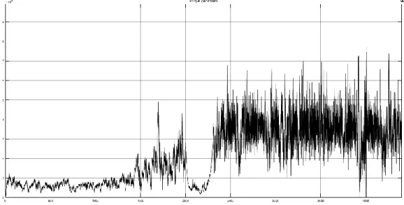
The model created after the training process comprises of the α,the sparse parameter, and the bias value b along with the kernel structure. The amount of memory space needed for storing it would be a parameter for the hardware feasibility of the proposed method. The memory space required for it be stored is around 160kb of the memory thus allowing it to be feasible in hardware implementation. By giving the different wind speed, which is randomly generation. Due to the variation in the wind the torque generated in the Figure 1.
Figure 1. Torque Waveform with random wind supply Turbine
The simulation is run for 4400 Secs. The faults are applied at different places like the below. 1.Fault type 1a, b1,m1 =-3o occurring between 100s and 200s.
2.Fault type 1b, b2,m2 =5o
2,m2 on 500-600s. 3.Fault type 1a, b3,m1 =7o on 900-1000s.
4.Fault type 2a, wr,m1 =2rad.s-1 on 1200-1300s.
5.Faults type 2b and 3b, wr,m2 =0.5wr,m2 and wg,m1 =1.5wg,m1 on 1700-1800s. 6.Fault type 4a, tg =tg -1000 Nm on 4200-4300s.
7.Fault type 6, hdt =0.22hdt
8. Fault type 5a, parameters in pitch actuator 2 (wn,z) 8 abruptly changed from [11.11, 0.6] to [5.73, 0.45] from 3200 and 3300s.
9. Fault type 5b, parameters in pitch actuator 3 (wn,z) changed slowly (with a linear function) from [11.11, 0.6] to [3.42, 0.9] over 30s, remained constant during 40s, and then decreased again over 30s from 3400 and 3500s.
While carrying out the training process the time taken for training all the fault and the non fault condition for all the nine fault conditions by using RVM is given in Table 2. After training the faults in the RVM implementation. The fault detection is tested with the above faults using the models developed using RVM.
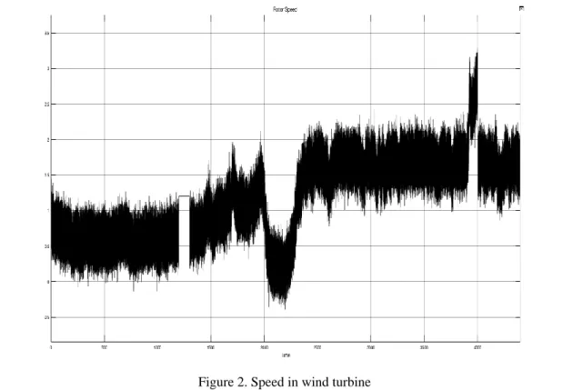
The detection of fault would show the 1 in the detection graph and zero in the detection graph when there is no fault. Figures 1 and 2 displays the wind turbine torque and the wind speed respectively in Turbine. Figures 3 and 4 displays the fault detected in Blade 1 and Blade 2 1200-1300s and 1700-1800s. The hardware feasibility of the proposed algorithm would require the time taken for the training portion and the memory space needed to store the models developed after the training process. The Table 2 displays the time taken for all the nine faults trained and the model generation for all the faults and the space for the models stored in the memory. The table is developed considering the i5 processor, 3.2GHz processor with the 8GB ram.
Table 2. Time taken for Training Each Faults Using RVM and Memory Used for the Model Thus Developed
Fault No. Fault Type Fault Site Memory Space for model Execution Time 1a Fixed Value Sensor Faults Blade Positions 16KB 1054 secs on an average for
each model 1b Gain Factor
2a Fixed Value Sensor Fault Rotor Speed 20KB 2b Gain Factor
3a Fixed Value Sensor Fault Generator Speed 10KB 3b Gain Factor
4a Offset Actuator Fault converter system 1KB 5a Abrupt Changed Dynamics Actuator Fault Pitch Systems 16KB 5b Slow Changed Dynamics 6 Changed Dynamics
System Fault Drive Train 47KB
Figure 3. Rotor speed fault detected in blade 1
Figure 4. Rotor speed fault detected in blade 2
4. CONCLUSION
The Relevance Vector Machine based implementation was carried out with the benchmark model developed as mentioned in the literature. The RVM function was trained and ten different models were developed for each kind of fault and the results were found to be satisfactory. The hardware feasibility study takes in to consideration the execution time and the memory usage for the models thus developed while training. The amount of execution time and the memory used clearly supports the hardware feasibility positively.
REFERENCES
[1] Odgaard, P.F., Stoustrup, J., and Kinnaert, M. “Fault tolerant control of wind turbines- a benchmark model,” IEEE Transactions on Control Systems Technology, Vol: 21, No.4, 1168 - 1182, July 2013.
[2] Santos, P, Villa, L.F, Reñones, A., Bustillo, A, Maudes, J, “An SVM-Based Solution for Fault Detection in Wind Turbines,” Sensors, 15, 5627-5648, 2015.
[3] Muhammad Rafi, Mohammad Shahid Shaikh, “A comparison of SVM and RVM for Document Classification,” ICoCSIM, Medan Indonesia, 2012.
[4] Mollasalehi, E, Wood, D, Sun, Q. “Indicative Fault Diagnosis of Wind Turbine Generator Bearings Using Tower Sound and Vibration,” Energies, 10, 1853, 2017.
[5] Anders BechBorcehrsen, JesperAbildgaardLarsen, JakobStoustrup, “Fault Detection and Load Distribution for the Wind Farm Challenge,” IFAC Proceedings Volumes, Volume 47, Issue 3, Pages 4316-4321, 2014.
[6] Seyed Mojtaba Tabatabaeipour and Peter F. Odgaard, and Thomas Bak, “Fault detection of a benchmark wind turbine using interval analysis,” American Control Conference Fairmont Queen Elizabeth, Montréal, Canada June 27-June 29, 2012.
[7] Xiukun Weiand LihuaLiu, “Fault detection of large scale wind turbine systems,” International Conference on Computer Science and Education (ICCSE),IEEE, 2010.
[8] Najim Aldin Mohsun, “Broken rotor bar fault classification for induction motor based on support vector machine-SVM,” Engineering& MIS (ICEMIS), 2017 International Conference on, February 2018.
[9] Qian Zhao et al, “Damage detection of wind turbine blade based on wavelet analysis,” Image and Signal Processing (CISP),2015 8th International Congress on 14-16, IEEE, Oct 2015.
[10] Mohanty, Soumya R., et al. "Comparative study of advanced signal processing techniques for islanding detection in a hybrid distributed generation system," IEEE Transactions on Sustainable Energy 6, 122-131, 1 2015.
[11] Thayananthan A., Navaratnam R., Stenger B., Torr P.H.S., Cipolla R. “Multivariate Relevance Vector Machines for Tracking. In: Leonardis A., Bischof H., Pinz A. (eds) Computer Vision-ECCV 2006,” Lecture Notes in Computer Science, vol 3953, Springer, Berlin, Heidelberg, ECCV 2006.
[12] Liyang Wei and Robert M. Nishikawa, “Relevance Vector Machine Learning for Detection of Microcalcifications in Mammograms,” IEEE, 2005.