Applications of Machine Learning for Predicting Selection Outcomes in Antibody Phage Display

Applications of Machine Learning for Predicting

Selection Outcomes in Antibody Phage Display

A Thesis Submitted to the

College of Graduate Studies and Research

in Partial Fulfillment of the Requirements

for the degree of Master of Science

in the Department of Computer Science

University of Saskatchewan

Saskatoon

By

Daniel Hogan

c

Permission to Use

In presenting this thesis in partial fulfilment of the requirements for a Postgraduate degree from the University of Saskatchewan, I agree that the Libraries of this University may make it freely available for inspection. I further agree that permission for copying of this thesis in any manner, in whole or in part, for scholarly purposes may be granted by the professor or professors who supervised my thesis work or, in their absence, by the Head of the Department or the Dean of the College in which my thesis work was done. It is understood that any copying or publication or use of this thesis or parts thereof for financial gain shall not be allowed without my written permission. It is also understood that due recognition shall be given to me and to the University of Saskatchewan in any scholarly use which may be made of any material in my thesis. Requests for permission to copy or to make other use of material in this thesis in whole or part should be addressed to:

Head of the Department of Computer Science 176 Thorvaldson Building 110 Science Place University of Saskatchewan Saskatoon, Saskatchewan Canada S7N 5C9

Abstract

Antibodies form an essential component of the adaptive immune system, but they also have important scientific and clinical applications. These applications exploit the proven ability of antibodies to bind strongly and specifically to nearly any biomolecular target (e.g. protein) of interest. To produce antibodies for scientific and clinical applications, researchers can use a wet-lab technique called antibody phage display. Antibody phage display starts with a library of diverse antibody fragments and selects and amplifies those fragments that bind to the target. Antibody phage display combined with next-generation sequencing (NGS) technology has the potential to yield greater insight into the selection process.

Machine learning is an area of artificial intelligence uniquely suited to recognizing patterns in large datasets, like those produced by NGS.

The research goals of this thesis were to (1) train machine learning models to predict the selection of antibody fragments in antibody phage display using only the sequence of the fragment; (2) validate the ability of the trained models to generalize to different experiments; and (3) reverse engineer the trained models to gain greater insight into the learned patterns and the selection process.

Antibody phage display data produced by the Geyer lab (University of Saskatchewan, SK) using two libraries called F and S was used to train a set of machine learning models: naive Bayes network (NB), linear model (LM), artificial neural network (ANN), support vector machine (SVM) with a radial basis function kernel (RBF-SVM), a SVM with a string kernel (SSK-SVM), and a random forest (RF). In addition, key parameters of the RBF- and SSK-SVM were tuned using a gridsearch. The trained models were then used to predict which antibody-displaying phage would be observed after the 5th round of panning, and their prediction accuracy on this data was used to help select models for subsequent analyses. The models selected were the RBF- and SSK-SVM. To achieve the second research goal, data originating from library F was used to train the two SVMs while library S data was used to test them. Finally, the two SVM models trained on library F were deconstructed to understand what features of the input correspond to negative predictions, and what features correspond to positive predictions.

The ANN, SVMs, and RF models had the best average classification accuracy (81.5%), but of this group, there was not one classifier that performed significantly better than the others. These classifiers could be used to help non-experts select clones from either library F or S for further wet-lab analyses.

The SVMs trained on library F and tested on library S achieved an average classification accuracy of 66.7%, significantly better than would be achieved by relying on chance. These two SVMs could be used to help non-experts select clones for further wet-lab analyses, provided the library being used is not too different from library S.

Finally, deconstructing the SVMs trained on library F yielded insight into the basis for their predictions. The predictions of the RBF-SVM were found to be highly dependent on the molecular weight of the relevant binding region (i.e. CDRH3).

Acknowledgements

There are many people I would like to thank for helping me complete this thesis. First, I would like to thank my supervisor, Dr. Tony Kusalik, for his guidance both when I was preparing for my graduate studies and during the completion of this thesis. I would also like to thank Bharathi Vellalore for helping me to understand antibody phage display, a central topic of this thesis. I would also like to thank Rahwa Zeresenai for her unwaivering support and encouragement over the past two years. Finally, I would like to thank my parents, Michael and Janie Hogan, for encouraging me to pursue my interests, which ultimately lead to the writing of this thesis.

Contents

Permission to Use i

Abstract ii

Acknowledgements iii

Contents iv

List of Tables vii

List of Figures viii

List of Abbreviations ix 1 Introduction 1 2 Background 4 2.1 Antibodies . . . 4 2.1.1 Overview . . . 4 2.1.2 Structure . . . 4

2.2 Antibody Phage Display . . . 7

2.2.1 Overview . . . 7

2.2.2 In Vitro Selection via Panning . . . 7

2.2.3 Antibody Library . . . 9 2.2.4 Panning Target . . . 9 2.3 Computational Biology . . . 9 2.3.1 Sequence Alignment . . . 9 2.3.2 Position-weight matrix . . . 11 2.3.3 Sequence Logo . . . 12 2.4 Machine learning . . . 12 2.4.1 Overview . . . 12

2.4.2 Training and learning . . . 13

2.4.3 Testing and validation . . . 13

2.4.4 Hyperparameters . . . 14

2.4.5 Machine Learning Techniques . . . 14

2.4.6 Related Machine Learning Applications . . . 21

2.5 Statistical Methods . . . 21

2.5.1 Wilcoxon Signed-Rank Test . . . 21

2.5.2 Friedman Test . . . 21

2.5.3 Mann-WhitneyU test . . . 22

2.5.4 Multiple Hypothesis Testing and the Bonferroni Correction . . . 22

2.6 Software . . . 22

2.6.1 MUSI . . . 22

3 Research Goals 24 3.1 Compare the Performance of Various Machine Learning Techniques in Application Area . . . 24

3.2 Assess the Generality of the Prediction Pipeline . . . 25

3.3 Present a Methodology for Interpreting the Trained Models . . . 25

4.1 Work Performed by the Geyer Lab . . . 26

4.2 Data Organization . . . 26

4.3 Feature Extraction . . . 28

4.3.1 Amino acid composition . . . 28

4.3.2 Dipeptide counts . . . 28

4.3.3 Physicochemical Properties . . . 29

4.4 Comparison of Machine Learning Techniques . . . 30

4.4.1 Overview . . . 30

4.4.2 Dataset Preparation . . . 30

4.4.3 Feature Selection . . . 30

4.4.4 Training and Validation . . . 31

4.4.5 Quantifying Prediction Performance . . . 31

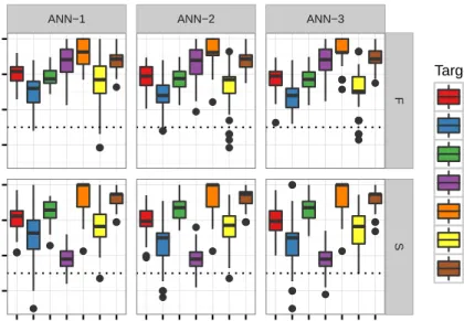
4.5 Improving ANN Classification Accuracy . . . 31

4.6 Improving SVM Classification Accuracy . . . 32

4.6.1 String Subsequence Kernel . . . 33

4.6.2 Gridsearch . . . 33

4.6.3 Comparing the Tuned SVMs to the Original Classifiers . . . 33

4.7 Cross-Library Validation of SVMs . . . 33

4.8 Interpreting the Trained SVMs . . . 34

4.8.1 Interpreting the Trained RBF-SVM . . . 34

4.8.2 Interpreting the Trained SSK-SVM . . . 34

4.9 Statistical Methods . . . 35

4.10 Hardware and Software . . . 35

5 Results & Conclusions 36 5.1 Preliminary Analysis . . . 36

5.1.1 MUSI Clusters and Sequence Logos . . . 36

5.1.2 Diversity over Panning Round . . . 36

5.1.3 Distribution of Physicochemical Properties . . . 38

5.2 Predicting Persistent Clones . . . 41

5.2.1 Feature Selection . . . 41

5.2.2 Cross-Validation . . . 41

5.2.3 Improving ANN Performance . . . 45

5.2.4 Optimizing SVM Parameters . . . 46

5.2.5 Comparing the Tuned SVMs to the Original Classifier Panel . . . 46

5.2.6 Conclusions . . . 46

5.3 Generalizing the SVM Models . . . 48

5.3.1 RBF-SVM Versus SSK-SVM Accuracy on Library S . . . 49

5.3.2 Conclusions . . . 49

5.4 Interpreting the SVM Parameters . . . 50

5.4.1 SSK-SVM . . . 50

5.4.2 RBF-SVM . . . 52

5.4.3 Conclusions . . . 52

6 Discussion & Future Work 59 6.1 Predicting Persistent Clones . . . 59

6.1.1 Machine Learning Comparison . . . 59

6.1.2 Improving SVM Performance . . . 60

6.2 Generalizing the Trained SVM Models . . . 60

6.2.1 SVM Performance on Library S . . . 60

6.3 SVM Models to Library Recommendations . . . 61

6.3.1 Features of the CDRH3 Sequences . . . 61

6.3.2 Dipeptide Compositions of the CDRH3 Sequences . . . 61

6.5 Training Data Quantity and Quality . . . 63

6.6 Contributions . . . 63

6.7 Future Work . . . 63

6.7.1 Feature Selection . . . 63

6.7.2 Alternative Classification Models . . . 64

6.7.3 Predicting Clone Abundance . . . 64

6.7.4 Target-Independent Method . . . 65

6.7.5 Size of the Training Dataset . . . 65

A Supplementary Figures 69 A.1 MUSI Clusters . . . 69

A.2 SVM Gridsearch . . . 72

A.3 Physicochemical Property Distributions . . . 73

A.4 RBF-SVM Support Vector Projections . . . 77

A.5 SSK-SVM Dipeptide Contributions . . . 80

List of Tables

2.1 CDR specifications for library F and library S . . . 10

2.2 Summary of protein targets. . . 11

2.3 Example Friedman test . . . 22

4.1 Example calculation of amino acid composition . . . 28

4.2 Example calculation of dipeptide counts . . . 29

5.1 Sequence logos for the clusters in samples F-Axl-5 and S-Axl-5 . . . 37

5.2 Sequence logos for the clusters in samples F-Mer-5 and S-Mer-5 . . . 38

5.3 The number of datapoints in each balanced dataset. . . 43

5.4 p-values from the Wilcoxon ranked-sum test comparing pairs of classifiers . . . 48

5.5 Dipeptides with the greatest contribution to each SSK-SVM mode . . . 56

A.1 Sequence logos for clusters in samples F-Jagged1-5 and S-Jagged1-5 . . . 69

A.2 Sequence logos for clusters in samples F-Jagged2-5 and S-Jagged2-5 . . . 70

A.3 Sequence logos for clusters in samples F-Notch1-5 and S-Notch1-5 . . . 70

A.4 Sequence logos for clusters in samples F-Notch2-5 and S-Notch2-5 . . . 71

A.5 Sequence logos for clusters in samples F-Notch3-5 and S-Notch3-5 . . . 71

A.6 Dipeptide contributions of the 7 SSK-SVM models. . . 80

List of Figures

2.1 PDB structure of an antibody . . . 5

2.2 Diagram of an antibody molecule . . . 6

2.3 In-vitro selection and amplification . . . 8

2.4 Sequence alignment example . . . 12

2.5 Example sequence logo . . . 12

2.6 Unsupervised machine learning example . . . 14

2.7 Best-first search example . . . 15

2.8 Decision tree example . . . 16

2.9 Example maximum-margin separating plane . . . 17

2.10 Substrings and subsequences in molecular biology . . . 19

2.11 Example artificial neural network . . . 20

2.12 A naive Bayes network. Nodes denote variables and arrows denote conditional dependencies between variables. . . 21

4.1 Terminology for antibody phage display samples . . . 27

4.2 ANNs with different numbers of hidden layers . . . 32

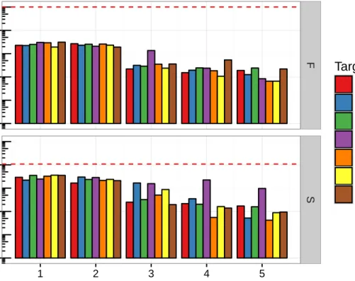
5.1 Log-scale barplot of phage sample diversity. . . 39

5.2 Log-scale barplot of phage sample diversity. . . 40

5.3 Distribution of length and aliphatic index across distinct clones . . . 42

5.4 Comparison of classifier accuracy . . . 44

5.5 Comparison of classifier accuracy . . . 44

5.6 Classification accuracy comparison for ANNs with different numbers of hidden layers . . . 45

5.7 Classification accuracy comparison for ANNs with different numbers of hidden layers . . . 47

5.8 Average performance of the RBF- and SSK-SVM using different parameters. . . 47

5.9 The effect of theγ parameters on the RBF . . . 48

5.10 Accuracy of the tuned SVMs and original classifier panel . . . 49

5.11 Improvement in accuracy by switching to tuned RBF-SVM . . . 50

5.12 Improvement in accuracy by switching to tuned SSK-SVM . . . 51

5.13 Accuracy of the trained RBF- and SSK-SVMs on the 7 library S datasets . . . 51

5.14 RBF-SVM support vector projections for the physicochemical properties . . . 53

5.15 RBF-SVM support vector projections for the amino acid composition . . . 54

5.16 RBF-SVM support vector projections for the dipeptide counts . . . 55

5.17 Dipeptide contributions for each of the 7 SSK-SVM models. . . 57

A.1 Full gridsearch results . . . 72

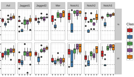
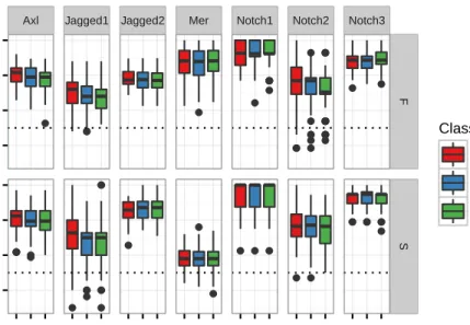
A.2 Violin plots showing the distribution of the aliphatic and Boman indices across the set of distinct clones identified in each sample . . . 73

A.3 The distribution of the charge and hydrophobicity across the set of distinct CDRH3 sequences identified in each sample . . . 74

A.4 The distribution of the instability index and isoelectric point across the set of distinct CDRH3 sequences identified in each sample . . . 75

A.5 The distribution of the length and molecular weight across the set of distinct CDRH3 sequences identified in each sample . . . 76

A.6 RBF-SVM support vector projections for the physicochemical properties . . . 77

A.7 RBF-SVM support vector projections for the amino acid composition . . . 78

List of Abbreviations

ANN artificial neural network CDRH1,2,3 heavy-chain CDR 1, 2, or 3 CDRL1,2,3 light-chain CDR 1, 2, or 3

CDR complementarity determining region CFS correlation-based feature selection ISP Ion sphere particle

MUSI multiple specificity identifier NGS next-generation sequencing RBF radial basis function SSK string subsequence kernel SVM support vector machine mAb monoclonal antibody pAb polyclonal antibody

Chapter 1

Introduction

The general aim of this thesis was to apply methods from an area of artificial intelligence called machine learning to a lab technology used for antibody discovery called antibody phage display. This introduction provides (1) a brief background for understanding this aim, (2) the motivation for this aim, (3) the research goals of this thesis, (4) an outline of the methodology of this thesis, and (5) an explanation of how this document is organized.

To defend against microbes and prevent infection, the human body is equipped with multiple layers of defence including the two main branches of the immune system: the innate immune system and the adaptive immune system. The innate immune system, evolving much earlier in history, recognizes molecular hallmarks of pathogenicity and responds to these hallmarks by sending cells and proteins to eliminate the hallmark-bearing pathogen. Some pathogens, however, do not carry any hallmarks that the innate immune system can recognize. To handle threats like these, vertebrates have evolved an adaptive immune system, which consists of specialized cells and proteins that recognize molecules that are not part of the organism. Proteins called antibodies play a pivotal role in this recognition mechanism.

Antibodies help the adaptive immune system distinguish self from non-self and focus resources toward eliminating the latter. The body is capable of producing a variety of antibodies that recognize the vast majority of non-self molecules. Even though each antibody only recognizes a specific molecular signature, the variety of antibodies produced by the body is so immense (roughly 1012 _{[1]) that, for any given target,} it is very likely that there exists an antibody that can bind to that target. Antibody structure and function, and clonal selection—the process the body uses to produce pathogen-fighting antibodies—is discussed in the background of this thesis (Section 2.1).

The ability of organisms to produce antibodies that bind strongly and selectively to proteins has been exploited to produce polyclonal antibodies (pAbs) for use in diagnostics (e.g. ELISA) and therapeutics. In addition to pAbs, there is great interest in developing monoclonal antibodies (mAbs). MAbs differ from pAbs in that all of the antibodies in a mAb originate from the same cell and are thus identical in sequence and structure, whereas the the antibodies in a pAb originate from different cells and are thus heterogeneous. MAbs are attractive because, among other reasons, they are easier to study and easier to reproduce [2].

Since the production of the first monoclonal antibodies in 1975 and the first FDA licence in 1986, mAbs have become an important weapon in the clinician’s arsenal [3]. Today, there are approximately 30 mAbs

approved by the FDA for treating human disease and conditions like cancer, chronic inflammatory diseases, transplantation rejection, infectious disease, and cardiovascular diseases [3]. The importance of mAbs is underscored by their global market value, which stands at approximately 20 billion USD per year; and the success of mAbs like Ramicade and Rituxan, which have annual sales exceeding 1 billion USD [4].

There are a variety of methods for developing mAbs with an affinity towards a target of interest. One such method is called antibody phage display. Antibody phage display uses bacterial viruses, called bacteriophage, to achieve clonal selection of target-binding antibodies in the lab. The procedure begins with a library of bacteriophage expressing antibody fragments on their capsid and carrying the corresponding gene in their genetic payload. In a process called panning, phage displaying target-binding antibody fragments are enriched by incubating the phage in a target-coated well, rinsing the unbound phage away, and then amplifying the immobilized target-bound phage by infecting a bacterial culture. A more detailed explanation of antibody phage display is given in Section 2.2.

One of the main goals of antibody phage display is to isolate phage that bind strongly, and specifically, to the target of interest. For therapeutic applications, target affinity is critical for increasing efficacy, reducing the required dosage, and easing side effects [5]. Because antibody phage display cannot generate antibody fragments that do not already exist in the library, the diversity of the initial library is critical to the success of the technique. Even if the library is sufficiently diverse and contains target-binding phage, antibody phage display may still fail due to other phage out-competing the target-binding phage, essentially masking them from discovery.

In order to understand library diversity and the enrichment process that happens during panning, studies have incorporated next-generation sequencing (NGS) [6, 7, 8]. NGS allows researchers to identify every sequence in a phage pool and approximate its concentration; however, to conduct an in-depth analysis on this data, intelligent and efficient computational methods are needed. Making sense of large datasets is a focus of machine learning. In addition, machine learning stresses computational efficiency and makes few assumptions about the process that gave rise to the data. An overview of machine learning as well as some of the specific techniques used in this thesis is given in Section 2.4.

This thesis will explore machine learning methods of leveraging NGS outputs from antibody phage display experiments with a view toward the following goals: (1) comparing the effectiveness of various machine learning techniques to this problem domain, (2) choosing the best machine learning method and validating its performance, and (3) demonstrating how machine learning can be used to inform the design of antibody libraries with enhanced specificity. These research goals are described further in Chapter 3.

To realize the goals of this thesis, NGS sequence outputs from real antibody phage display experiments conducted by the Geyer lab were processed to make them suitable for input to machine learning methods. A software package called Weka was used to train various machine learning methods for the task of predicting whether or not a specific clone will be observed after 5 rounds of panning given the CDRH3 sequence of that clone. Cross-validation was used to compare the performance of the machine learning methods and hone in

on one of the best techniques, called Support Vector Machines, which is described in Section 2.4.5. The SVMs were trained to predict outcomes of antibody phage display and then they were dissected to understand the basis for their performance and to suggest ways of modifying the antibody phage display library to improve specificity toward the targets used in the experiments. A complete description of the methodology is given in Chapter 4.

Listed in order, this thesis includes the following chapters: Background, Research Goals, Methodology, Results & Conclusions, and Discussion & Future Work. Background will overview theory, techniques, and literature that are necessary to understand the rest of the text. Research Goals states the specific objectives of this thesis. Methodology lays out the work that was done to complete the research goals, and provides the necessary detail for reproducing the work. Results & Conclusions presents the observations and con-clusions made during execution of the methodology. Discussion provides general commentary including the implications of the results, conjectures, and directions for future work.

Chapter 2

Background

2.1

Antibodies

2.1.1

Overview

To avoid infection the human body must fight off microbes like viruses, bacteria, and parasites and to mount a defence against these pathogens, the body must have the capacity to distinguish them from self-molecules. A big part of this recognition mechanism is the responsibility of proteins called antibodies.

Antibodies are symmetrical Y-shaped proteins capable of recognizing and binding specific molecular sur-faces (called epitopes) with two of its three branches (called the variable regions). During the development of antibody-producing cells, called B-cells, the antibody-coding genes of these cells are systematically ran-domized so that each B-cell produces its own antibody variant that recognizes a unique molecular surface. Because the number of antibody variants produced by this randomization process is so immense, the body has the capacity to produce antibodies that recognize nearly any molecular surface. To eliminate antibodies that are self-reactive and leave only those that react to foreign molecules, B-cells producing antibodies that are self-reactive are culled out in a process called negative selection. The result is an antibody repertoire that reacts to almost any threat but not to the body [9].

To accommodate such a large diversity of antibodies, the concentration of each antibody in the body is minuscule. In response to an infection, the body uses a process called clonal selection to increase the concentration of antibodies that bind to the invading pathogen. The process of clonal selection depends on the cells that produce antibodies, called B-cells. In addition to producing free-floating antibodies, a B-cell is decorated with membrane-bound proteins resembling antibodies, called B-cell receptors (BCRs). When a suitable antigen binds to a BCR, the BCR sends a signal to the B-cell that causes it to proliferate. As the B-cell proliferates, it also upregulates the production of antibodies. In this way, only antibodies that can actually aid in the battle against the invading pathogen are actually produced [9].

2.1.2

Structure

A detailed view of an antibody molecule is shown in Figure 2.1. Conceptually, the structure of an antibody has the shape of the letter Y. This Y is composed of four chains: two identical heavy chains (Hc) and two

Figure 2.1: Structure of an antibody [10, 11]. Heavy chains are coloured red and light chains are coloured yellow.

identical light chains (Lc). The C-terminal halves of both heavy chains associate to form the stem of the Y while the N-terminal halves are divided between the two top branches, each associating with one of the light chains (Figure 2.2a) [9].

The parts of an antibody can be classified based on their function within the molecule. In order of increasing specificity, these regions are Fc, Fab, Fv (Figure 2.2b), and CDRs. The Fc region refers to the stem of the Y and is also called the constant fragment because it is identical in every antibody. The Fc region is also the part that is recognized and bound by other components of the immune system. The two remaining branches of the Y-shaped antibody are called Fabs, or antibody binding fragments. Within each Fab is the Fv region, also called the variable region. Finally, at the N-terminal tip of the Fv region resides the CDRs (complementarity determining regions). The CDRs are six loops (three from the heavy chain and three from the light chain) which are responsible for sticking to the molecular surface of the antigen (termed the epitope). Three of these CDRs (CDRH1, CDRH2, and CDRH3) come from the heavy chain. The other three (CDRL1, CDRL2, and CDRL3) come from the light chain. Antibody diversity is created by randomizing the genes encoding these loops. The reader can learn more about antibodies in the text by Sompayrac [9].

(a) Antibody molecule coloured by chain. Heavy chains are coloured blue and light chains are coloured green.

Fab

Fc

Fv

(b)Antibody molecule coloured by region. The con-stant region (Fc) is shown in green, the Fabs are shown in red (light and dark), and the variable re-gions (Fv) are shown in dark red.

Antigen

(c) An antibody bound to an antigen. The surface making contact with the antigen is formed by the 6 CDRs (not shown) of the variable region. The surface of the antigen making contact with the antibody is called the epitope.

2.2

Antibody Phage Display

2.2.1

Overview

The observation that (1) human antibodies are well-tolerated by the body, (2) antibodies are highly specific to their target, and (3) an antibody can be made for any given target, has lead to a great investment in using antibodies for research, diagnostics, and therapeutics [3]. Much of the interest in antibodies is focused on monoclonal antibodies (mAbs). A mAb is a collection of antibodies that are identical copies, or clones, of one another. To avoid confusion, in the remainder of this document, the term clone means “a collection of identical antibodies”. This definition will replace the alternate meaning of the word, which is “a single copy of an antibody”. For example, a mAbs consists of a single clone, whereas polyclonal antibodies (pAbs), which are heterogeneous collections of antibodies, consist of multiple clones.

Antibody phage display is a lab technique used for developing mAbs with affinity toward targets of interest. Whereas the proliferation of antigen-binding antibodies within the human body is an example of in vivo clonal selection, antibody phage display is a method for in vitro clonal selection. Antibody phage display exploits the biology of bacteriophage (viruses that infect bacteria) to achieve this selection.

2.2.2

In Vitro

Selection via Panning

Antibody phage display begins with a library: a collection of phage-antibody hybrids displaying antibody fragments on their surface. An antibody phage display library typically contain over 1010 _{different clones} [12], comparable to the diversity of the human antibody repertoire. One might then expect that, for a given target, there exists an antibody in the library that can bind to that target. Such a hypothesis is tested using a selection process called panning. Panning has three basic steps: incubate, wash, and amplify. When conditions are ideal, these steps enrich target-binding phage. Panning can be repeated a number of times to achieve further enrichment. In the incubation step the phage are pipetted into target-coated wells. With time, phage that display antibodies with target-affinity become immobilized on the surface of the well. The next step is to rinse the well several times to wash away any unbound phage. With separation of bound and unbound phage achieved, the final step is to either recover the DNA of the phage or to amplify the bound phage remaining in the well so that further enrichment steps can be completed. Amplification is achieved by infecting a suitable bacterial culture.

Sequencing of the antibody fragments present in the phage results in thousands to millions of sequences in which a number of highly redundant sequences can be found. Barring sequencing errors, each set of redundant sequences come from a set of identical phage, called clones. The general idea is that the more abundant a sequence, the more abundant the clone, and thus the higher affinity that clone has for the target. Next-generation sequencing of antibody phage display samples is common [6, 7, 8]. The reader can find an overview of phage display in the work of Carmen & Jermutus [14].

Figure 2.3: A pool of Fab-phage are selected and amplified to enrich those that bind to the target (also called the antigen). (1) A pool of Fab-phage are incubated in an antigen-coated well; (2) Unbound Fab-phage are removed by washing the well with solution, leaving Fab-phage that bound the antigen; and (3) the antigen-bound Fab-phage are eluted from the antigen and amplified in an E. coli host. The process can be repeated to further enrich antigen-binding Fab-phage [13]

2.2.3

Antibody Library

In antibody phage display, a population of phage is called a library. One common, albeit simplistic, metric for the quality of a library is its diversity, or number of distinct clones. Some state-of-the-art libraries have estimated diversities of over 1010 _{clones, rivalling the diversity of the human antibody repertoire [12].}

Libraries are constructed with DNA coding for antibody fragments with diverse variable regions. Each DNA fragment is then inserted into a vector coding for a bacteriophage capsid protein such that the expression product of the vector is a fusion protein between the capsid and the antibody fragment. The recombined vector is then transfected into a bacterial culture infected with the same type of bacteriophage. During virion assembly, the fusion protein is incorporated into the phage capsid alongside the wild-type capsid proteins, producing bacteriophage that display the antibody fragment on their surface. Moreover, the DNA of the vector contains specific signals that allow it to be packaged within the phage progeny. The result is bacteriophage carrying the DNA of the antibody that decorates their surfaces. The linkage between antibody DNA and antibody fragment turns out to be crucial forin vitro selection [14].

The DNA used to construct antibody phage display libraries can be derived from the antibody repertoire of an organism, or synthesized using a template antibody and a suitable mutagenesis technique. Constructing an antibody library synthetically offers greater control over the makeup of the constructed library. The CDRs of synthetic libraries can be made to follow a specific design. For example, the libraries studied in this thesis, library F and library S, were constructed synthetically according to the specification shown in Table 2.1 [14].

Library F is a synthetic antibody phage display library that uses a constant antibody framework and variable CDR-H1, H2, H3, and L3, with most diversity focused toward CDR-H3. The length of CDR-L3 and H3 varies from 8 to 12 residues and 7 to 23 residues, respectively. Library S was designed around library F, but unlike library F, contains no variability in CDR-H1 and H2, and has a CDR-H3 that can vary in length from 7 to 25 residues. The specification for library F and library S is shown in Table 2.1 [13].

2.2.4

Panning Target

In antibody phage display, the molecule one wishes to develop an antibody for is called the target. Seven protein targets used in experiments carried out by the Geyer Lab are shown in Table 2.2.

2.3

Computational Biology

2.3.1

Sequence Alignment

Biological sequences, such as DNA and proteins, are easily represented using strings of symbols (i.e. sequences of characters). For example, the DNA sequence consisting of the bases

guanine-adenine-thymine-thymine-Table 2.1: CDR specifications for library F and library S. One-letter abbreviations are used to signify amino acids. Brackets signify that any of the contained amino acids may appear at the position in the sequence. Superscripts denote repetitions in the sequence.

CDR Library Specification L1 F RASQSVSSAVA L1 S RASQGISNYLA L2 F YSASSLYS L2 S YAASSLQS L3 F QQ[YSGAFWHPV]3-7_[PL][IF]T L3 S QQ[YSGTAPHREFWVL]4_PLT H1 F AASGFN[IL][YS][YS][YS][YS][IM]H H1 S AASGFTFSSYGMH H2 F [YS]I[YS][PS][YS][YS][SG][YS]T[YS] H2 S VISYDGSNKY H3 F AR[YSGAFWHPV]1-17_[AG][FLIM]DY

H3 S AR[YSGTAPHREFWVL]1-10_{[AGDY]FDY and} AR[YSGAFWHPV]7-15_{YYYY[GY][MF]DV}

Table 2.2: Summary of protein targets.

Short Name Full Name Gene Description [15]

Axl Tyrosine-protein kinase receptor AXL Cell signalling receptor that helps regulate cell survival, cell prolif-eration, migration, and differen-tiation.

Jagged1 Protein jagged-1 JAG1 Ligand for Notch receptors. Be-lieved to affect cell-fate decisions during hematopoiesis.

Jagged2 Protein jagged-2 JAG2 Ligand for Notch receptors. Af-fects limb, craniofacial, and thymic development.

Mer Tyrosine-protein kinase Mer MERTK Cellular signal receptor that reg-ulates cell survival, migration, differentiation, and phagocytosis. Notch1 Neurogenic locus notch homolog protein 1 NOTCH1 Receptor for 1 and

jagged-2 (see JAG1/JAGjagged-2).

Notch2 Neurogenic locus notch homolog protein 2 NOTCH2 Receptor for 1 and jagged-2 (see JAG1/JAGjagged-2).

Notch3 Neurogenic locus notch homolog protein 3 NOTCH3 Receptor for 1 and jagged-2 (see JAG1/JAGjagged-2).

adenine-cytosine-adenine can be represented as the string “GATTACA”. This unambiguous representation is easily manipulated by computers, which enables computers to carry out useful biological operations like sequence alignment.

Sequence alignment is usually carried out to determine whether two sequences are similar enough to assume they share some characteristic (e.g. evolutionary history, protein structure, function etc.). In silico, determining how similar two sequences are is carried out by finding the alignment which maximizes an objective function called the scoring function. The scoring function expresses, in formal terms, how good an alignment is. The resulting alignment can itself be represented as two strings, one shown above the other as in Figure 2.4a. Sequence alignment can be performed on more than two sequence. Such an alignment is called a multiple sequence alignment (MSA). An example of an MSA is shown in Figure 2.4b.

2.3.2

Position-weight matrix

A position-weight matrix (PWM) is one way to represent a MSA. In a position-weight matrix, the rows represent each of the 20 amino acids and the columns represent each position in the MSA. The value stored in the element at row iand columnj is the probability of observing amino acidiat positionj of the MSA.

G A T T A C A | | | | ATTA -G A T T A C A ||| | - ATT - - A (a) G A T T A C A ATTA -GA - T A C A (b)

Figure 2.4: (a) Two possible alignments of the DNA sequence ATTA with the DNA sequence GAT-TACA. A priori, the first alignment is better because it does not contain internal gaps. (b) A multiple sequence alignment of the DNA sequences GATTACA, ATTA, and GATACA.

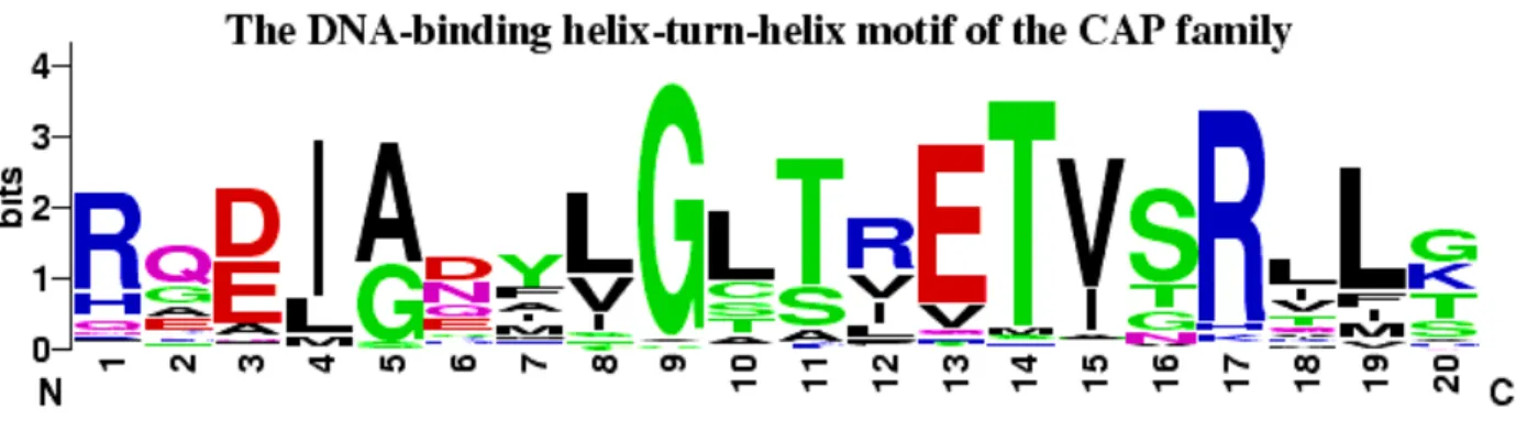
Figure 2.5: An example of a sequence logo [16].

2.3.3

Sequence Logo

A sequence logo is a visualization of an MSA. An example is shown in Figure 2.5. A sequence logo shows the positions of the MSA along a horizontal axis. Above each position, a number of pictures are stacked vertically. Each picture in the stack depicts a single symbol, but the symbol is stretched or squashed to occupy a specific amount of vertical space. The vertical space occupied by the picture signifies the probability in bits (₋log2P) of observing the depicted symbol at the corresponding position in the MSA.

2.4

Machine learning

2.4.1

Overview

In data analysis, one deals with sets of repeated measurements, e.g. species, petal length, and petal width for each iris in a garden. In their entirety, these measurements form a dataset.

The measurements in a dataset are often dealt with mathematically as vectors, e.g. an iris of species versicolor having a petal length of 1.400_{, and a petal width of 0.2}00_{can be encoded as the 3-dimensional vector}

N-dimensional space, whereN is the number of measurements associated with the observation. Thought of this way, the observation is called a datapoint.

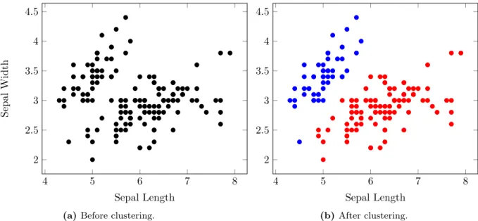
Machine learning deals with the development and application of algorithms that extract meaningful patterns from large datasets. Sometimes these patterns reveal hidden structure in the dataset. Looking for these kinds of patterns is dealt with in the area of unsupervised machine learning. An example of unsupervised machine learning is shown in Figure 2.6. Other times, these patterns are used to predict the unknown attributes from partial observations, e.g. predicting the species of an iris from its petal length and width. Looking for these kinds of patterns is dealt with in the area of supervised machine learning [17].

To predict unknown attributes, supervised machine learning techniques use a function or combination of functions that takes a datapoint as input and outputs a number or label. This number or label output by the model becomes the prediction for the unknown attribute. Before the model can make reasonable predictions, however, it must first be trained with a dataset. Training allows the model to learn apparent relationships between the known attributes, also called predictor variables, and the unknown attributes, also called response variables.

Supervised machine learning can be further separated into classification and regression problems. A regression problem arises when the response variable is continuous (in the mathematical sense). An example of a regression problem is trying to predict the height of an individual based on a set of genetic predictors. A classification problem arises when the response variable is categorical (i.e. can be enumerated). An example of a classification problem would be trying to diagnose a patient as either infected or healthy based on a set of clinical observations.

2.4.2

Training and learning

The functions that make up a machine learning model contain a number of adjustable parameters that affect the predictions the model makes. A training algorithm is an optimization procedure that adjusts these parameters in order to minimize the prediction error on the training dataset. For example, in a linear model having the form y =mx+b, the slope m and y-interceptb are the parameters that are optimized during linear regression, a sort of training algorithm.

2.4.3

Testing and validation

After training a machine learning model on the training dataset, it is necessary to test the model on another dataset, called the testing dataset. The purpose of testing is to show that the model has not simply learned to remember the training dataset, but has actually learned meaningful patterns that generalize to observations outside of the training dataset.

4 5 6 7 8 2 2.5 3 3.5 4 4.5 Sepal Length Sepal Width

(a) Before clustering.

4 5 6 7 8 2 2.5 3 3.5 4 4.5 Sepal Length (b)After clustering.

Figure 2.6: A hypothetical example of unsupervised machine learning. (a) The initial data consisting of two measurements: sepal length and sepal width. The initial data was subjected to clustering, which tries to divide the data into well-defined groups. (b) The same data coloured red or blue according to the clusters identified by a clustering procedure.

2.4.4

Hyperparameters

In addition to normal parameters, which are optimized during training, machine learning models often have parameters which can be set by the user. These parameters are called hyperparameters. Hyperparameters can have a broader impact on the resulting model than normal model parameters. An important consideration in machine learning is finding the hyperparameter values that work best for a particular problem.

2.4.5

Machine Learning Techniques

Correlation-Based Feature Selection

In machine learning, raw input is often processed into a smaller set of variables, called features, which are then fed into the machine learning tool to predict the response variable. The processing of raw input into features is called feature extraction.

For a given prediction task, there may be features that do not correlate well with the response variable. These features are said to be noisy. There may also be features that correlate so well with each other that their combined predictive power is worth no more than the predictive power of each feature alone. These features are said to be redundant. Correlation-based features selection (CFS) is a procedure invented by Mark A. Hall [18] that selects noisy and redundant features to discard.

The main contribution of CFS is a method for measuring the merit of a feature set. The method uses an equation that measures the average correlation between each predictor and the response variable, but

penalized for correlation between predictors. CFS can handle not only continuous variables but ordinal, nominal, and binary variables as well.

The Weka interface to CFS provides a number of common search strategies for finding the features that maximize the CFS equation. One of these search strategies—the one used in this thesis—is called best-first search.

The best-first search implementation can start with either (1) the empty set of features or (2) the set of all features. In this thesis, the empty set of features was used, so only this method will be described but before best-first search is described, some basic terms and concepts need to be defined:

Child: A feature set Ais said to be the child of another feature setB ifAcontains all of the features of B plus one more.

Expansion: The expansion of a feature set is the enumeration of all its children.

Best-first starts by expanding the empty set (e.g. Figure 2.7a). Expansion of the empty set results in the discovery of a number of features sets, each containing only a single feature. The search continues by choosing the best unexpanded set to expand next (e.g. Figure 2.7b). The search stops when 5 consecutive expansions do not improve upon the CFS score of the best set. When the stopping criteria is met, the algorithm returns the best set that was discovered.

{} {a} {b} {c} (a) {} {a} {b} {a, b} {b, c} {c} (b)

Figure 2.7: (a) The empty feature set is expanded, resulting in the discovery of three new feature sets. (b) The feature set with the best CFS score (_{b_}) is expanded, resulting in the discovery of two more feature sets.

Decision Trees and Random Forests

A decision tree is a classifier that uses a structured set of rules for classifying new instances (Figure 2.8). To classify a datapoint using a decision tree, the rule at the root of the tree is applied first. If the rule is satisfied, the next rule applied is the left descendent of the root, otherwise it is the right descendent. This proceeds down the tree until a leaf node is reached. The label contained in the leaf node becomes the predicted class of the datapoint.

A decision tree can be built to correctly classify every datapoint in a dataset; however, the ability of such a tree to generalize to other data is typically poor. A random forest is an attempt to counteract the poor generality of a decision tree. A random forest is a collection of decision trees, each trained on a different subset of the training data [19]. After training, the random forest contains a collection of decision trees that are d ifferent, yet are trained to do the same thing. By averaging over the predictions of each decision tree, a classifier that is less prone to overfitting results (i.e. less dependent on the training data).

For random forests, bagging and random feature selection are two methods for injecting randomness into the training of each decision tree. In bagging, the training dataset is resampled before training each decision tree. In random feature selection a random subset of features is used to train each decision tree [20].

Expression correlation>0.9? Shared cellular localization? False No Genomic distance<5kb False No True Yes Yes No Shared function? False No True Yes No

Figure 2.8: A hypothetical decision tree for deciding whether a pair of proteins interact [21].

Logistic Model

A logistic model is a prediction tool used for binary classification problems. The two classes of a binary classification problem will be called the positive and negative classes. The input to a logistic model is a set of numeric variables and the output is a number between 0 and 1 that approximates the probability that the input belongs to the positive class. For a given input, if the logistic model produces a value of 0.5 or greater, the model predicts that the input belongs to the positive class; otherwise, the model predicts that the datapoint belongs to the negative class. A logistic model is trained by maximizing the likelihood function of the model. The likelihood function expresses the probability that the model generates the observed data, and is described in the text by Witten and Frank [19].

x y v1 v2 v3 (a) x y v1 v2 v3 (b)

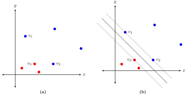
Figure 2.9: An example of a maximum-margin separating plane. (a) Datapoints with two variables represented on thexandy axes. The red dots belong to one class and the blue dots belong to another. (b) The maximum-margin separating plane shown as a solid black line. Datapoints labelled v1, v2, andv3 are the support vectors of this plane. The margin is the space between the two dotted black lines.

Support Vector Machine

A support vector machine (SVM) is a popular machine learning model used for binary classification problems. SVMs can be understood by first visualizing data as coloured points ink-dimensional space, where the colour denotes the class of the data point and the value on each of thekaxes is the value of each of thekpredictor variables (Figure 2.9a). The goal in training an SVM is to find the maximum-margin separating plane, which is the plane that separates points of different colours such that there is a maximum amount of space between the plane and the points (Figure 2.9b). Visually, if the plane has a thickness, the goal is to find the thickest plane that separates the points. Once the maximum-margin separating plane is found, predictions for new datapoints depend on what side of the plane the new datapoint falls. The reader can learn more about SVMs in the text by Alpaydin [17].

Support vector machines get their name from the fact that the maximum-margin separating plane can be defined in terms of a subset of the datapoints in the training dataset, called the support vectors. The decision to classify a new data point as belonging to either the positive or negative class is made based on the result of a linear combination of the inner-products between the new data point and each of the support vectors. For example, in Figure 2.9b, the datapoints labelled v1, v2, and v3 are the support vectors of the maximum-margin separating plane; the maximum-margin separating plane is defined completely by these 3 datapoints.

In addition to linear separating planes, support vector machines can classify using non-linear surfaces by mapping the training data into another space with a special function and then performing the training procedure in this new space. This mapping can be achieved implicitly by substituting the inner-product in the decision function with another function. These functions are called kernels.

For real classification problems, separating all of the datapoints into their respective classes with a plane may be impossible. For this reason, most SVMs use a soft-margin, which allows some of the training data to be misclassified. The parameter C is introduced to control the balance between (1) the goal of making the margin as large as possible, and (2) the soft-constraint that all training data be on the correct side of the plane and outside of the margin [22]. Lowering the value ofC softens the constraint, but the value ofC must remain positive.

Radial Basis Function

One example of an SVM kernel is a radial basis function (RBF). A RBF is shown in Equation 2.1, whereγ is an adjustable parameter andxandx0 _{are two vectors. Intuitively, the RBF kernel is a similarity function}

that maps pairs of vectors into the interval [0,1]. The RBF kernel is at a maximum (equal to 1) when the pair of vectors are equal. As the distance between the vectors increases, the RBF kernel decays to 0. γ controls how fast a RBF decays and must be positive.

K(x,x0) = exp(₋γ_||x₋x0_||) (2.1) When fed a vector as input, a RBF-SVM classifies the vector through the following procedure: For each support vector, the RBF-SVM calculates the distance to the input vector, multiplies this distance by ₋γ, then takes the exponential of the result. The resulting term is multiplied by the weight of the support vector. Finally, the RBF-SVM sums the resulting terms and adds a constant term, which was also learned during training. If the sum is positive, the RBF-SVM classifies the input as positive; otherwise, it classifies the input as negative.

Strings, Subsequences, and the String Subsequence Kernel

A string is a sequence of symbols from a predefined alphabet. For example, a DNA sequence is a string that is made from the symbols A, T, G, and C. A substring of a string sis a string that can be made into sby adding symbols to either end. A subsequence of a string s is a string that can be made into s by adding symbols anywhere in the string. For example, consider the string s= GATTACA. ATTA is a substring ofs but ATTC is not; however, ATTC is a subsequence ofs.

In the context of molecular biology, DNA or amino acid sequences can be represented by strings. A substring of a stringscan therefore be thought of as an ungapped local alignment onsthat does not contain mismatches. Likewise, a subsequence can be thought of as a local alignment on s that does not contain

s F T F T A L I L L A V A V | | | | | | s0 _TALILL -(a) s F T F T A L I L L A V A V | | | | | | s00 _TALILL -s F T F T A L I L L A V A V | | | | | | s00 _{T ALILL} -(b)

Figure 2.10: Substrings and subsequences in a molecular biology context. (a) A substrings0 ofsis an ungapped local alignment ofs0 _{ontosthat contains no mismatches. (b) A subsequences}00 _{ofsis a}

local alignment ofs00_{ontosthat contains no mismatches and only contains gaps in thes}00 _{part of the}

alignment.

mismatches and only contains gaps in the subsequence part of the alignment. Examples of a substring and subsequence in this context are shown in Figure 2.10.

The string subsequence kernel (SSK) is a more exotic SVM kernel because it operates on strings instead of vectors [23]. Intuitively, the SSK is the number of subsequences shared between two strings and weighted by the number of gaps in the shared subsequences. The SSK kernel is parameterized by two parameters, the decayλ and the subsequence lengthn. Intuitively, the decayλdetermines how much shared subsequences are penalized for containing gaps.

Artificial Neural Network

An artificial neural network (ANN) is a machine learning tool composed of nodes and edges. An example of a small ANN is shown in Figure 2.11. The nodes in an ANN are processing units which sum together signals from adjacent nodes, apply a function, and send the resulting signal to nodes further down the network through its outgoing edges. The edges in an ANN not only connect node outputs to node inputs, but also multiply the signals they carry by a weight.

In feedforward ANNs (the kind of ANN used in this thesis) nodes are organized into layers, where the first layer contains nodes that receive the input, and the final layer contains nodes that produce the output. The layers in between the input layer and output layer are called hidden layers. Every node in layer i is connected to every node in layeri+ 1. In addition, each layer has a bias node capable of shifting the entire signal up or down. Figure 2.11 shows an example of a feedforward ANN.

The goal of training an ANN is to find values for the edge weights that minimize the prediction error of the ANN with respect to the training dataset. This minimization problem has no direct mathematical solution, but a numerical procedure called gradient descent can find values that are locally optimal.

Gradient descent requires initial values for the edge weights. The initial values may be supplied by the user and drastically affect the outcome. Using the initial values, the direction of steepest descent is determined by taking the derivative of the training error with respect to each edge weight. Each edge weight is then adjusted

0,0 0,1 0,2 0,3

1,0 1,1 1,2 1,3 1,4

2,1

Figure 2.11: An example of a small artificial neural network. Nodes are labelled x, ywhere xand y denote the layer and node, respectively. By convention, layer 0 is the input layer and node 0 is the constant bias. The nodes in the input layer (shown in blue) take on the values of the predictor variables. The signal propagates down the edges to adjacent nodes. At each edge the signal is multiplied by a weight. At each node the signals are added together, transformed with the activation function, and sent through the outgoing edges. Eventually the signal reaches the output node (shown in red) which predicts the value of the response variable.

to move in this direction by a certain amount. The size of this step is determined by the learning rate. The gradient descent process is often compared to the trajectory of a ball that has been placed randomly on a curved surface. The ball has a random initial position (the initial edge weights) and the elevation of the ball (the training error) is determined by the surface (the training error). The ball moves in the direction of steepest descent, eventually stopping at the bottom of the basin. By analogy, the edge weights move in the direction of steepest descent (with respect to the training error) and stop when the edge weights reach values where any movement, no matter the direction, increases training error. Optionally, a momentum may also be introduced to allow the ball to roll against the direction of descent and jump from one basin to another. The reader can learn more about ANNs in the text by Bishop [24].

Naive Bayes Network

A naive Bayes network is a simple machine learning model in which every predictor variableX is assumed to be conditionally dependent on the response variable Y but independent of all the other predictor variables. Naive Bayes networks are trained by estimating the conditional probability (P(X_|Y)) for each predictor variable using maximum likelihood estimation [19]. A trained naive Bayes network is used for prediction by applying Bayes’ rule (Equation 2.2). The graph of a naive Bayes network is shown in Figure 2.12.

P(Y_|X) =P(X|Y)P(Y)

Y

X1 X2 · · · Xn

Figure 2.12: A naive Bayes network. Nodes denote variables and arrows denote conditional depen-dencies between variables.

2.4.6

Related Machine Learning Applications

Machine learning has many fruitful applications in the field of molecular biology. One example is the detection of CpG islands with hidden Markov models [25]. Another example is the prediction of protein secondary structure from protein sequence using artificial neural networks [26]. A third example is the prediction of interacting protein pairs using random forests [27]. Machine learning has also been used in drug development for screening millions of drug candidates for those that are likely to fail [28].

2.5

Statistical Methods

Statistical tests allow one to support or refute hypotheses by deferring to statistical probabilities.

2.5.1

Wilcoxon Signed-Rank Test

The Wilcoxon signed-rank test is a non-parametric (i.e. distribution-free) test that can be used to compare the medians of two related samples. The samples must be related in the sense that there is a natural way to pair the data. An example of two such samples arises when a medical intervention is being tested on a patient group and measurements are taken before and after the intervention. In this example, the pre-intervention measurements form one sample, and the post-intervention measurements form the other. In addition, the measurements in both samples can be paired according to the patient they came from. Pairing the samples has the advantage of controlling for variables that differ between patients.

Using the example of the previous paragraph, the Wilcoxon signed-rank test helps answer the question “are the measurements taken after the intervention consistently higher (or lower) than the measurements taken before the intervention?” [29].

2.5.2

Friedman Test

If the data can be tabulated like the example shown in Table 2.3, the Friedman test can be used to test the hypothesis that the observations in one or more of the rows are statistically higher (or lower) than the other rows, while controlling for variables that differ between columns. The Friedman test is similar to the Wilcoxon signed-rank test except that the Friedman test is not limited to pairs of datapoints. The drawbacks

Table 2.3: The grades receieved by 3 students in the subjects math, science, and english. The Friedman test could be used to test the hypothesis that one or more students received statistically higher (or lower) marks than the others.

Student Math Science English

A 65 50 95

B 60 70 90

C 80 85 60

of the Friedman are that (1) it is less sensitive than the Wilcoxon signed-rank sum test (i.e. more likely to falsely accept the null hypothesis) and (2) it does not indicate which row is dominant [29].

2.5.3

Mann-Whitney

U

test

Like the Wilcoxon signed-rank test, the Mann-WhitneyU test can be used for comparing two samples, except that the samples do not need to be paired [29].

2.5.4

Multiple Hypothesis Testing and the Bonferroni Correction

If, instead of a single hypothesis, a group of hypotheses are being tested using a dataset, the probability of falsely rejecting a null hypothesis increases in proportion to the number of hypotheses. Using the example from Section 2.5.1, such a situation might arise if, instead of testing one intervention, multiple interventions are being tested.

One way to account for the increased chance of error associated with multiple hypotheses is to use the Bonferroni correction [29]. The Bonferroni correction ensures that the change of falsely rejecting a single null hypothesis is less than the significance levelα.

2.6

Software

2.6.1

MUSI

Clustering is one example of unsupervised machine learning. The goal of clustering is to find groups (i.e. clusters) of datapoints that are similar to each other but different from datapoints in other groups. An example application of clustering is classifying patients diagnosed with a particular disease into disease sub-types based on clinical observations and disease outcomes.

MUSI (Multiple Specificity Identifier) [30] is a software package that performs clustering on a set of short peptide sequences. The MUSI algorithm first performs a mulitple sequence alignment (Section 2.3.1) on the peptide sequences before selecting a set of PWMs (Section 2.3.2) to represent the MSA. The selection procedure returns the maximum number of PWMs (fit using expectation maximization) that satisfy the

MUSI criteria: (1) each PWM (i.e. cluster) has enough sequences and (2) no two PWMs are too similar. Each PWM returned by the selection procedure corresponds to a single cluster.

Chapter 3

Research Goals

Next-generation sequencing has enabled scientists to examine the DNA of biological systems (e.g. hu-mans, eukaryotes, bacteria, viruses, and environments) with unprecedented detail. With the high volume of information produced by NGS, however, comes the oft-cited challenge of storing, organizing, processing, and analyzing this sequence data. Comprehending such high volumes of data is impossible to do manually. Not excluded from these difficulties is the area of antibody phage display, where phage populations containing millions of genetically distinct clones can be characterized in a single NGS run, allowing researchers equipped with the right tools to perform an in-depth analysis of the sequence landscape present within the population. The deluge of sequence data produced by applying NGS to antibody phage display presents a unique challenge to the computational biologist. Each sequenced sample provides a detailed snapshot of the make-up of the contained phage; but the factors that account for changes in the population observed between snapshots is understood primarily on a qualitative level. While this high-level understanding coupled with the researcher’s own experience has been sufficient to bring about major advances in the field [31], there is still opportunity to bring to bear machine learning techniques to this exciting new area.

The aim of this thesis is to explore applications of machine learning to antibody phage display in the following context: Given the sequence of a clone and a target, can the presence or absence of a clone after the 5th panning round be predicted? As the presence or absence of a clone in the third, fourth, and fifth rounds of panning is one of the first criteria the analyst uses in selecting clones for further experimentation, this prediction task is a good candidate for machine learning.

The aim of this thesis was distilled into three research goals, which are presented in the following three sections (Sections 3.1 to 3.3).

3.1

Compare the Performance of Various Machine Learning

Tech-niques in Application Area

The field of machine learning is rife with techniques for learning complex patterns from data and making predictions based on those learned patterns [17, 24, 19]. No single technique is strictly dominant, but each has areas of application where it excels. The first research goal of this thesis is to develop a general methodology for applying different machine learning models to the prediction task at hand, and then to

use this methodology to compare the classification accuracy of a variety of machine learning models. The general methodology must prescribe methods for (1) identifying and extracting informative features from the CDRH3 sequence data and (2) tuning the hyperparameters of the models.

3.2

Assess the Generality of the Prediction Pipeline

The usefulness of a trained machine learning model depends crucially on its ability to generalize to data not observed in the original training set, a concept called generality. The second research goal is to determine to what extent the best machine learning technique (chosen based on the results from the previous research goal) can generalize to antibody phage display experiments that use different libraries. Such a finding would suggest that the selected machine learning technique can find relationships between a clone’s CDRH3 sequence and its outcome that are independent of the library.

3.3

Present a Methodology for Interpreting the Trained Models

Decisions for library construction are made on the basis of experience, intended targets, and resources. Libraries may go through an iterative process of improvement by altering the original specification or con-struction protocols. Machine learning models vary in their explanatory power; that is, the ease at which their predictions can be understood in terms of the material inputs. By reverse engineering the learned classifier in the prediction pipeline, general properties can be derived which correlate with the experiment outcomes and the fate of clones. These properties can be interpreted as a prescription for further specialization of the antibody library into a focused antibody library. The third goal of this thesis is to develop one possible methodology for extracting this information from the learned models.

Chapter 4

Data & Methods

4.1

Work Performed by the Geyer Lab

Using antibody phage display, the Geyer Lab [13] selected clones from library F and library S for affinity to seven targets named Axl, Jagged1, Jagged2, Mer, Notch1, Notch2, and Notch3 (Table 2.2). Screening was carried out in a series of 14 antibody phage display experiments, each experiment using a different library-target combination. To achieve sufficient enrichment of library-target-binding clones, 5 rounds of panning were used in each experiment. After each round of panning, samples of the resulting phage population were sequenced using an Ion Torrent sequencer.

For sequencing, the Geyer Lab [13] amplified the CDRH3 region of selection outputs (phage samples) using designed primers; then performed emulsion PCR on the amplicons using proprietary Ion sphere particles (ISPs); and finally sequenced the enriched ISPs on an Ion semiconductor chip. The sequences output by Ion Torrent were prepared for data analysis with a sequence of steps that included the removal of reads that diverged significantly from the library specification and reads with a low overall quality.

Because the sequenced samples form the basis of the following analysis, an unambiguous terminology for referring to different collections of them was devised. Samples can be identified uniquely by the library, target, and panning round from which they were collected; therefore, they can be said to form a 3-dimensional array with library, target, and panning round represented on the 3 axes. Figure 4.1 shows this 3-dimensional representation. Using this analogy, when an analysis is described as being performed on the S-Notch3 sample array, samples from S-Notch3 rounds 0-5 are implied (Figure 4.1b).

For a typical sample, thousands of sequences were identified, many of which were identical. It was assumed that identical sequences came from identical clones and that the number of identical sequences was proportional to the concentation of that clone.

4.2

Data Organization

The CDRH3 DNA sequences produced by the Geyer Lab were translated into amino acid sequences using thetranseqprogram from the EMBOSS package [32]. The resulting protein sequences were inserted into a PostgreSQL [33] table calledreads. The sequences in thereadstable were grouped by the sequence, library,

F S Axl Jagged1 Jagged2 Mer Notc h1 Notc h2 Notc h3 0 1 2 3 4 5 Library Target Round

(a)Library S-Notch3-Round 1 sample.

F S Axl Jagged1 Jagged2 Mer Notc h1 Notc h2 Notc h3 0 1 2 3 4 5 Library Target Round

(b)Library S-Notch3 sample array.

Figure 4.1: The phage samples viewed as a 3-dimensional array of cubes. (a) The sample collected following round 5 of panning Library S against Notch3, denoted S-Notch3-5. (b) The samples collected in all Library S versus Notch3 panning rounds, denoted S-Notch3.

target, and round columns; and then counted. These unique entries were inserted, along with their counts, into a table called clones.

The reason for managing data with a DBMS like PostgreSQL was two-fold: (1) PostgreSQL ensures that the entered data is valid and (2) querying a flatfile requires that, at worst, the entire file first be read, a time-consuming operation, whereas PostgreSQL stores data in a native binary format which is designed for rapid retrieval of information.

4.3

Feature Extraction

The sequences in the clonestable were preprocessed to extract a diverse collection of potentially informa-tive features. These features can be divided into 3 groups. The first of these groups contains the amino acid compositions of the 20 amino acids (Section 4.3.1). The second contains the counts of each dipeptide (Section 4.3.2). The third contains a variety of physicochemical properties (Section 4.3.3). After extracting these features, a preliminary analysis was conducted to gain a better understanding of the data.

4.3.1

Amino acid composition

The amino acid composition of a clone was the fraction of the clone’s variable CDRH3 sequence made up by each of the 20 possible amino acids. An example calculation is shown in Table 4.1.

Table 4.1: Calculating the amino acid composition for the sequence YYYYVYDFDY. Amino Acid Sequence Composition

D YYYYVYDFDY 0.2

F YYYYVYDFDY 0.1

V YYYYVYDFDY 0.1

Y YYYYVYDFDY 0.6

4.3.2

Dipeptide counts

The dipeptide counts for a clone were the number of each of the 384 different dipeptides present in the clonal variable CDRH3 sequence. Out of the 400 possible dipeptides, 16 were omitted from this set of features because they were not observed in any of the sequenced samples. A sequence of length l contained l₋1 dipeptides, so the sum of the dipeptide counts for a clone with a sequence of length l was equal to l−1. Calculating the dipeptide counts for the sequence YYYYVYDFDY is shown in Table 4.2.

The motivation for using dipeptide counts instead of fractions was based on an analogy with binding motifs in protein sequences. Let X be a well-known binding motif for target T and let A and B be two proteins that haveX in their sequence. Also, assume that the number of amino acids in proteinB is half the number in proteinA. In this hypothetical scenario, knowing how many timesX occurs in A or B is more relevant than whether these proteins bind toT than knowing the fraction ofAorB made up byX because the answer does not depend on the size of the protein. Following the analogy, if a dipeptide is viewed as a micro-motif of the CDRH3, which can vary is size, then the question of how many times that dipeptide

occurs in the CDRH3 is more informative than the question of what fraction of the sequence is made up by that dipeptide.

Table 4.2: Calculating the dipeptide counts for the sequence YYYYVYDFDY. Sequence Dipeptide YYYYVYDFDY YY YYYYVYDFDY YY YYYYVYDFDY YY YYYYVYDFDY YV YYYYVYDFDY VY YYYYVYDFDY YD YYYYVYDFDY DF YYYYVYDFDY FD YYYYVYDFDY DY

(a)Decomposing the sequence into dipeptides.

Dipeptide Count YY 3 YV 1 VY 1 YD 1 DF 1 FD 1 DY 1

(b)Counting the dipeptides.

4.3.3

Physicochemical Properties

In addition, a collection of physicochemical properties were estimated for each clone’s sequence. These features included the following eight physicochemical properties, calculated using the R package Peptides (version 1.1.1) [34].

Aliphatic index: From Ikai [35]: “The relative volume of a protein occupied by aliphatic side chains (ala-nine, valine, isoleucine, and leucine).”

Boman index: The average solubility value of the amino acids in the sequence.

Charge: The net charge of the sequence.

Hydrophobicity: The average hydrophobicity index of the amino acids in the sequence.

Instability Index: An index of how rapidly a protein will degrade. A protein that has an index less than 40 is considered stable (e.g. has a very long half life) [36].

Length: The number of amino acids in the sequence.

Molecular weight: The combined molecular weight of the amino acid sequence.

4.4

Comparison of Machine Learning Techniques

4.4.1

Overview

Each clone that was observed after 5 rounds of panning received a label of persistentand each clone that was observed in the naive library, but not after round 5 received the labeltransient. A panel of classifiers was trained to classify clones as eitherpersistentortransientbased on the clonal sequence. The panel of classifiers consisted of a logistic model (LM), random forest (RF), support vector machine (SVM), artificial neural network (ANN), and naive Bayes network (BN). Although by no means exhaustive, this list of classifiers covers many of the popular machine learning classifiers used today. Using Weka [37], each classifier in the panel was trained and tested on the features calculated for each library-target sample array. Because there were 2 libraries, 7 targets, and 5 different classifiers, the analysis consisted of 70 subanalyses (2_×7_×5).

4.4.2

Datas