Nonlinear system identification and control using dynamic multi-time scales neural networks

Nonlinear System Identification and Control tisi

Dynamic Multi-Time Scales Neural Networks

Xuan Han

A Thesis

In

The Department of

Mechanical and Industrial Engineering

Presented in Partial Fulfillment of the Requirements

for the Degree of Master of Applied Science (Mechanical Engineering) at

Concordia University Montreal, Quebec, Canada

April, 2010

?F?

Your file Votre référence

ISBN: 978-0-494-67204-4

Our file Notre référence

ISBN: 978-0-494-67204-4

NOTICE:

The author has granted a

non-exclusive license allowing Library and Archives Canada to reproduce, publish, archive, preserve, conserve, communicate to the public by

telecommunication or on the Internet, loan, distribute and sell theses worldwide, for commercial or non-commercial purposes, in microform, paper, electronic and/or any other formats.

The author retains copyright ownership and moral rights in this thesis. Neither the thesis nor substantial extracts from it may be printed or otherwise reproduced without the author's permission.

AVIS:

L'auteur a accordé une licence non exclusive permettant à la Bibliothèque et Archives Canada de reproduire, publier, archiver, sauvegarder, conserver, transmettre au public par télécommunication ou par l'Internet, prêter, distribuer et vendre des thèses partout dans le monde, à des fins commerciales ou autres, sur support microforme, papier, électronique et/ou autres formats.

L'auteur conserve la propriété du droit d'auteur et des droits moraux qui protège cette thèse. Ni la thèse ni des extraits substantiels de celle-ci

ne doivent être imprimés ou autrement reproduits sans son autorisation.

In compliance with the Canadian Privacy Act some supporting forms may have been removed from this thesis.

Conformément à la loi canadienne sur la protection de la vie privée, quelques formulaires secondaires ont été enlevés de cette thèse.

While these forms may be included in the document page count, their removal does not represent any loss of content from the thesis.

Bien que ces formulaires aient inclus dans la pagination, il n'y aura aucun contenu manquant.

¦+¦

Abstract

Nonlinear System Identification and Control using Dynamic

Multi-Time Scales Neural Networks

In this thesis, on-line identification algorithm and adaptive control design are proposed for nonlinear singularly perturbed systems which are represented by dynamic neural network model with multi-time scales. A novel on-line identification law for the Neural Network weights and linear part matrices of the model has been developed to minimize the identification errors. Based on the identification results, an adaptive controller is developed to achieve trajectory tracking. The Lyapunov synthesis method is used to conduct stability analysis for both identification algorithm and control design. To further enhance the stability and performance of the control system, an improved dynamic neural network model is proposed by replacing all the output signals from the plant with the state variables of the neural network. Accordingly, the updating laws are modified with a dead-zone function to prevent parameter drifting. By combining feedback linearization with one of three classical control methods such as direct compensator, sliding mode controller or energy function compensation scheme, three different adaptive controllers have been proposed for trajectory tracking. New Lyapunov function analysis method is applied for the stability analysis of the improved identification algorithm and three control systems. Extensive simulation results are

provided to support the effectiveness of the proposed identification algorithms and

control systems for both dynamic NN models.

Acknowledgements

This thesis is finished during the research in the Mechanical and Industrial Engineering Department of Concordia University. It is a great opportunity to study here. I am very grateful to all the professors, technicians and fellow students whom I have worked with in this research field.

Firstly, I would like to express my deep gratitude to my supervisor Dr. Wenfang Xie. She provides me with the inspiration and direction in my research. Critical feedback from

her keeps me progress throughout my graduate education. Her enthusiasm, creativity and

concentration dramatically inspired me to improve the quality of the research and conquer the difficulties.

Secondly, I am deeply indebted to the colleagues and friends in Montreal for their help and advices.

Finally, I would like to thank my parents for always believing in me.

Xuan Han

Montreal Canada

Table of Contents

List of Figures vii

List of Tables ix

List of Symbols, Abbreviations and Nomenclature ?

Chapter 1 Introduction 1

1.1 Motivation 1

1 .2 Literature review . 3

1 .2.1 Overview of system identification 3

1.2.2 Development of control strategies for nonlinear systems 7 1.2.3 NN-based nonlinear system identification and control 8

1.2.4 Multi-time scale system 12

1.2.5 Identification and control of systems with multi-time scale 15 1.3 Research objectives and main contributions of this thesis 16

1.3.1 Research objectives 16

1.3.2 Main contributions 16

1 .4 Thesis Outline 17

1.5 Conclusion 17

Chapter 2 Mechanism and Structure of Neural Network 19

2.1 Feedforward neural network 19

2.2 Dynamic Neural Network 20

2.3 Multi-Time Scales Neural Networks... 24

2.4 Conclusion 28

Chapter 3 Identification and Control for nonlinear systems with multi-time scales 29

3.1 On-line Identification 29

3.1.1 Nonlinear systems with multi-time scale 29

3.1.2 Dynamic NN model 30

3.1.3 Adaptive Identification Algorithm 31

3.1.4 Simulation Results of identification 36

3.2 NN-based adaptive control design 50

3.2.1 Tracking error analysis 50

3.2.2 Simulation results of control scheme 54

3.3 Conclusion 56

Chapter 4 Improved NN based Adaptive Control Design 57

4.1 Improved system identification 57

4.1.1 Identification with precise structure of NN identifier 58 4.1.2 Identification for nonlinear systems with bounded un-modeled dynamics 66

4.1.3 Simulation results 74

4.2 Multiple control methods based on Neural Network 80

4.2.1 Tracking Error Analysis 80

4.2.2 Improved controller design 83

4.2.3 Simulation result ,. 89

4.3 Conclusion 93

Chapter 5 Conclusion and future work 94

List of Figures

Figure 1-1 DC Servomotor 13

Figure 2-1 Structure of MLP 20

Figure 2-2 Structure of recurrent neural network 21

Figure 2-3 Threshold function 23

Figure 2-4 Piecewise-Linear function 23

Figure 2-5 Sigmoid function 24

Figure 2-6 Structure of dynamic neural network with two time-scales 25

Figure 2-7 Hyperbolic Tangent Function 26

Figure 2-8 Structure of modified dynamic neural network with two time-scales 27

Figure 2-9 Logistic Function with multi-parameters 27

Figure 3-1 Identification scheme 34

Figure 3-2 Identification result for X| 37

Figure 3-3 Identification result for ?? in [15] 37

Figure 3-4 Identification error for xj 38

Figure 3-5 identification resuit for x2 38

Figure 3-6 Identification result for X2 in [15]... 39

Figure 3-7 Identification error for X2 39

Figure 3-8 The eigenvalues of the linear parameter matrices 40

Figure 3-9 Identification result for ? 41

Figure 3-10 Identification error for X] 42

Figure 3-1 1 Identification result for X2 , 42

Figure 3-12 Identification error for X2 43

Figure 3-13 The eigenvalues of the linear part matrices 43 Figure 3-1.4 The learning process of the updating weight matrices 44

Figure 3-15 Identification results 47

Figure 3-16 Eigenvalues of the linear matrices A, B 48

Figure 3-17 Identification results 48

Figure 3-18 Eigenvalues of the linear matrices A, B 49

Figure 3-19 Identification and control scheme 51

Figure 3-20 Trajectory tracking of ? 55

Figure 3-21 Trajectory tracking of y 55

Figure 4-1 Improved Identification Scheme 66

Figure 4-2 Identification result for Xi 75

Figure 4-3 Identification error for Xi 75

Figure 4-4 Identification result for X2 76

Figure 4-5 Identification error for X2 76

Figure 4-6 The eigenvalues of the linear parameter matrices A, B 77

Figure 4-7 Identification results in Case A 78

Figure 4-8 Eigenvalues of the linear matrices A, B in Case A 78

Figure 4-9 Identification results in Case B 79

Figure 4-10 Eigenvalues of the linear matrices A, B 79

Figure 4-1 1 New Identification and control scheme 82

Figure 4-12 Trajectory tracking results using direct compensation 90 Figure 4-13 Trajectory tracking results using Sliding Mode Compensation 91 Figure 4-14 Trajectory tracking results using energy function compensation 92

List ©f Tables

Table 3-1 Sigmoid function parameters 41

Table 4-1 Sigmoid function parameters 75

Table 4-2 RMS for Control 93

List of Symbols, Abbreviations and Nomenctatyre

Artificial Neural Network Single Input Single Output Multi-Input Multi-Output Multilayer Perceptron Radial Basis Function

Dynamic Multi-Time Scales Neural Networks

Hodgkin-Huxley Root Mean Square

Extremely Low Frequency Back Propagation

State variable of Neural network Output layers weight

Hidden layers weight Activation function Activation function Control input Linear part matrix

e Singular Perturbation Parameter

/(·) Input-output mapping function

_* TTÏ-* TT7* TT?"*

W1 ,W2, W3, W4 Nominal constant matrices

A , B Nominal Hurwitz matrices

AXjjAv Identification error

?/? ' A/>

Modeling error and disturbances

V1 Lyapunov function for Identification

A, B Updating law of linear part matrix

"?,2,3?4 Updating law of output layers weight

a Compensation positive constant

Vc

Lyapunov function for control

? Eigenvalue

?, Ax , Ay Positive definite matrix

ax,ßx,ay,ßy

?p function

yAyB Eigenvalue of linear part matrix

RMS Root mean square

xd, yd Desired Trajectory

E? >Ey

Tracking control error

?/? ¦> A/ ?

Upper bound ofmodeling error

S? >$y Dead-zone indicator

H H¦I'" V Identification threshold

Chapter 1 Introduction

1.1 Motivation

Numerous systems in the industrial fields demonstrate nonlinearities and uncertainties which can be considered as partial or total black-box. Dynamic neural networks have been applied in system identification and control of those systems for many years. Due to the fast adaptation and superb learning capability, the dynamic neural networks have

transcendent advantages compared to the static ones [14], [15].

A wide class of nonlinear physical systems contains slow and fast dynamic processes

that occur at different moments. Recent research results show that neural networks are

very effective for modeling the complex nonlinear systems with different time-scales when one has incomplete model information, or even when the plant is considered as a

black-box [14].

Dynamic neural networks with different time-scales can model the dynamics of the short-term memory of neural activity levels and the long-term memory on dynamics of unsupervised synaptic modifications [21]. The stability of equilibrium of competitive neural network with short and long-term memory was analyzed in [22] by a quadratic-type Lyapunov function. In [23-25], new methods of analyzing the dynamics of a system with different time scales are presented based on the theory of flow invariance. The K-monotone system theory was used for analyzing the dynamics of a competitive neural

system with different time scales in [26].

Since system identification and control using dynamic neural networks (NN) was first introduced systematically in [27], the past decade has witnessed great activities in

stability analysis, identification and control with continuous time dynamic neural networks with or without considering the time scales. In [28], Sandoval et al. developed new stability conditions by using a Lyapunov function and singularly perturbed technique. In [29], the passivity-based approach was used to derive stability conditions for dynamic neural networks with different time-scales. The passivity approach was used to prove that a gradient descent algorithm for weight adjustment was stable and robust to any bounded uncertainties, including the optimal network approximation error [8]. Many dynamic neural networks-based direct and indirect adaptive control algorithms for regulation and tracking have been published in the literatures [10, 30, and 31]. With consideration of the uncertainty of dynamic systems, the indirect method that adopts

on-line identification via neural networks followed by controller design is developed and

widely used. Several papers proposed adaptive nonlinear identification and trajectory [9] or velocity [11] tracking via dynamic neural networks without considering the multiple

time scales. However, the above mentioned research has concentrated on the stability

analysis instead of control for dynamic systems by using dynamic neural networks with time-scales or developed control scheme based on the neural network without

considering time-scales.

In this thesis, on-line identification for nonlinear system with uncertainties using multi-time scales dynamic neural network are developed and then various controllers are designed for trajectory tracking based on the on-line identification results.

1.2 Literature review

1.2.1 Overview of system identification

Since the modeling and parameter estimation are initiated by the mathematical statistics and time series analysis, many disciplines like economic, social science and engineering have participated and contributed to this field. In 1956, Zadeh first introduced the term-System Identification for the problem of identifying a black box by its input-output relationship [32]. Since then, a lot of researches have been devoted to system identification which has become an established branch of control theory. Since systems with unknown linear parameters or unknown nonlinear characteristics cannot be controlled optimally, to identify these unknown linear parameters and nonlinear

characteristics is essential in control domain. System identification is a process of

estimating the architecture and parameters of a model from the input and output data. From different points of view, system identification can be classified as on-line and off-line identification, or grey box and black box, or off-linear system and nonoff-linear system

identification.

a) ' On-line and Off-lime identification

Conducting estimation process after collecting the data from the system are known as Off-line identification. On the contrary, these two steps are running at the same time for on-line identification. The main advantages of on-line identification are that the specified

precision can be achieved by recursive process and real time identification for time

varying system. Model reference techniques of the on-line identification problem are

employed filtered version of the recursive least-squares as identification algorithm [35]. In [36], Kaiman proposed a linear-quadratic estimator called Kaiman filter. The extended Kaiman filter is used to system identification problems of seismic structural systems in

[37].

b) Black-box and grey box

Depending on the level of prior knowledge, the identification model can be catalogued into two groups. If absolutely no information about the process is available, the identification plants are notated as black-box. For the other cases, grey-box refers to the situations that considerable knowledge of the structure and/or parameters are already

known.

For linear single input single output (SISO) Black-box models, Ljung summarized the general family structure which can rise to 32 different models [38].

F{q) D(q)

A(q) = ì + aìq~ì+... + annq~"a

B{q) = \ + bxq-i+... + bubq-"b

(U)

C(q) = l + a]q~i +... + aiicq~"c

D{q) = \ + a]q'i+... + andq""1

F(q) = l + alq~i +... + aiifq-"'

where u(t) and y(t) are scale input and output signal for a system, q is forward shift

operator defined as qu(t) = u(t + \) and q~[ is backward shift operator defined as

q~\i{t) = u{t-\).

FIR - Finite Impulse Response (A=C=D=F=I )

ARX- AutoRegressive with Exogenous input (C=D=F=I) ARMA - AutoRegressive Moving Average (B=D=F=I )

ARMAX - AutoRegressive Moving Average model with Exogenous inputs model

(D=F=I)

ARARX - AutoRegressive AutoRegressive with Exogenous input (C=F=I )

OE- Output Error (A=C=D=I) BJ - Box-Jenkins (A=I)

Recently the research results show that these methods have been extended for Multi-input Multi-output (MIMO) system. An identification algorithm using FIR model is proposed for multi-input, multi-output stochastic systems [49]. New evolutionary programming method is proposed to identify the ARMAX model for short term load forecasting [52]. Monin has derived a new identification algorithm for OE and ARMAX systems with exogenous nonstationary multiple input based on a hereditary computation [53]. Model identification and diagnostic checking using BJ method are developed for the control of prostheses for varied limb function, movement and circumstances [54].

The regressors for nonlinear system identification are similarly selected, hence the names are inherited with adding "N" representing nonlinear at beginning, like NFIR, NARX, NARMAX NOE and NBJ. In [55], NFIR Volterra model are utilized for a subspace approach of blind identification and equalization of nonlinear single-input

multiple-output system. NARX time series are investigated with projections for

nonlinear ARMA identification algorithm is developed based on affine geometry. It is

faster for the new algorithm to obtain the estimation results than the fast orthogonal search method. Subspace algorithms with a basis function are applied to identify a Hammerstein model expansion which is followed by modeling Wiener nonlinearity to

build a model for ionospheric dynamics [56].

c) Linear system and nonlinear system identification

Linear systems obviously represent the most vita group of system identification. After years of extensive development in practice and in the literature, linear system identification techniques have been systematically presented in text books. Even though, there are still some improvement which are made for the past few decades. In [43],

Guillaume et. al. discussed and analyzed a mathematical model of the Empirical Transfer

Function Estimate with noisy input signals which is not deterministic and exactly known for Fourier analysis. Tugnait proposed a frequency-domain solution to the least-squares equation error identification problem using the power spectrum and the cross-spectrum of the time-domain input-output data to estimate the parametric input-output infinite impulse response transfer function [44]. Overschee and Moor find state-space models by subspace state space system identification algorithms from the input and output data [46] .

Before 1980s, system identification techniques for nonlinear systems have received

scant attention due to their inherent complexity and difficulty. As nonlinear systems are

widely engaged in many different research fields, like control application, artificial intelligence, pattern recognition, signal processing etc., nonlinear system identification

Compared to linear systems, it is very difficult to obtain the precise physical model

for nonlinear system and more distinct structural models can be chosen. On the other hand, the models need not to be true and accurate description of the real system. It is just a description of some of its properties to serve certain purpose [38]. Hence, many researchers tend to use reduced-order or linear model to represent the system. Transient

response method is used to model the reduced-order transfer functions of power converters by analyzing the step response [39]. Linear models of Tokamak are created for control purpose and validating different models from physics principles by frequency response identification [40]. A continuous-time nonlinear unstable magnetic bearing systems are successfully identified by using a linear model and frequency response data

[41].

Jean-Marc and René investigated the identification using nonlinear autoregressive

models [47]. Volterra series serves as a generalization of the convolution integral to model a seventh order nonlinear model of a synchronous generator with saturation effect [48]. Nonlinear system identification is conducted by Reduced Volterra model with generalized orthonormal basis functions, which can overcome the huge estimation process [49]. Singh and Subramanian established a direct correspondence between the

structure of a nonlinear system and the pattern of its frequency response [42].

1.2.2 Development of control strategies for nonlinear systems

Linear control as a mature topic with various effective methods has been systemically

presented in textbook and successfully operated in industrial applications. In early age of development of control engineering, not a wide range of nonlinear analysis tools are

available for researchers and engineers as today. Before 1940, some immature nonlinear control methods, like Tirrill regulator and the fly-ball governor have been successfully applied without systematically theoretical analysis [57]. Phase plane method, describing function method and Tsypkin's method for relay systems as the major nonlinear system analysis techniques during the two decades since 1940s are also discussed in [57]. Then the control engineering community boosts attention to Lyapunov's stability theory after more than 60 years since it is first published in 1892. Lyapunov's direct method has become the most fundamental and popular nonlinear system analysis tool for the major

nonlinear control system design methods.

1.2.3 NN-based nonlinear system identification and control

When dealing with non-linear systems as well as linear systems with multiple inputs and multiple outputs, traditional identification methods need specific assumptions concerning the model structure. It is usually assumed that the system equations are known except for a number of parameters [45]. Neural networks have been proven to be effective for nonlinear system identification and control due to highly complexity and

nonlinearity.

a) Static networks and dynamic networks

The architectures of neural networks can be categorized into two fundamental classes: feedforward (static) networks and recurrent (dynamic) networks. The major difference

between them is that recurrent NN has at least one feedback loop.

identification and control [4, 5, 6]. A typical example is the multilayer perceptron (MLP), which is utilized to identify the dynamic characteristics of a nonlinear system. The main characteristic of MLP—fast convergence makes it prime candidate for adaptive control of nonlinear systems. In [64], MLP NN is used to realize the position control of a Low Earth

Orbit satellite. RBF neural networks are artificial neural networks with radial basis

functions as activation functions. Similar to feedforward neural networks, RBFs are

widely used in function approximation, time series prediction, control, pattern recognition and classification. Mark gave a systematic introduction about RBF neural networks [66]. RBF neural networks were also applied for diagnosis of diabetes mellitus [67], whose performance is evaluated with MLP neural networks and logistic regression. After comparing the performances of a multilayer MLP network and a RBF network for the online identification of a synchronous generator, Jung-wook et. al. claimed that the RBF network is simpler to implement, needs less computational memory, converges

faster and better even in the changing operating conditions [65].

On the other hand, the recurrent neural networks have received considerable attention in recent two decades. Due to their strong nonlinear characteristics, dynamic NNs are

more and more widely used for nonlinear system identification and control. On-line system identification based on modified recurrent neural network NARX model with three different validation algorithms are presented to serve the predictive controller [68].

Based on a recurrent neural network uncertainty observer, a back-stepping and adaptive

combined controller is designed to perform position control of an induction servomotor [69]. The recurrent neural networks are trained based on the experimental data from a

continuous biotechnological process for system identification and control [70].

Identification result of a class of control affine systems are used to synthesize the

feedback linearization of the system which then can be controlled by a PID controller

[71].

b) Learning algorithm

All the neural network topologies are supported by their corresponding training or learning algorithms. Years ago, back propagation is the dominating learning algorithms since it is first introduced by Paul J. Werbos in 1974 [7]. In addition, many efforts have been made to improve the traditional back propagation approach. New back propagation algorithm with optimization process for the slope of sigmoid function at each neuron is presented in [58], which accomplishes faster convergence rate and better accuracy model, especially for high level nonlinear systems, comparing to traditional back propagation method for system identification with neural networks. Various improved back propagation algorithm are presented for recurrent neural networks in [60]. An accelerated back propagation can remove the delay when the error is back-propagated through the adjoin model. Predictive back propagation and targeted back propagation with or without filtering are studied to update the weights of the network. Yue-Seng and Eng-Chong investigate various aspects like net pruning during training, adaptive learning rates for individual weights and biases, adaptive momentum, and extending the role of the neuron in learning and then combing them together to improve the performance of back propagation for multilayer feed-forward neural networks [61].

proposed for system identification and control purpose. Widely discussed recently are Evolutionary algorithms which can optimize neural network architecture to provide faster training speed [76]. In [62], evolutionary neural networks are proposed by combining the immune continuous ant colony algorithm and BP neural network. Structure and weights

of static or recurrent neural networks can be simultaneously acquired by presented

evolutionary programming [63]. In [59], a cascade learning architecture is developed to provide dynamic activation functions for neural networks. This results in faster learning

speed, smoother process and simpler structure of the networks when it is used for

identifying human control strategy. c) Applications and experiment

There are numerous reports regarding the successful application and experiment of NN-based controllers in the real systems. The multi-loop nonlinear neural network tracking controller is implemented for a single flexible link [72]. Neural network

controller combined with PID controller is tested on a wheeled drive mobile robot based

inverted pendulum to maintain balance as well as track desired trajectories [73]. In [74], a 2-degrees-of-freedom inverted pendulum on an x-y plane is controlled by a decentralized

neural network control scheme. Each axis is controlled by two separate neural network controllers since the decentralized controller can not only compensate the uncertainties

but also decouple the system. In a word, numerous training processes are fast enough,

1.2.4 SVIuIti-time seal© system

Numerous nonlinear physical systems contain slow and fast dynamic processes that

occur at different moments. The following models are used to describe such dynamic characteristic of the nonlinear systems.

a) Singularly perturbed system

We consider a system of ks+k2 first-order autonomous ordinary differential equations for k{ +k2 dynamic variables, of which kt are slow variables and k2 are fast

variables. Therefore the vector of slow variables is x, e Rkì and the vector of fast

variables x2 e Rkl . Then the system of equations is

dx

—*¦ = /; (x,, X2)

M

(1.2)

at

which is a slow-time system. e > Ois a small parameter. System (1.2) has asymptotic structure (kx,k2) .

The transformation of time t = e? brings this system to the form of a fast-time system:

-^ = £/¡(x,,x2)

dl

¦

(1.3)

-^ = ZJ(XpX2)

Systems (1.2) and (1.3) are equivalent to each other for finite e , but have different properties in the limit e -> O+ .

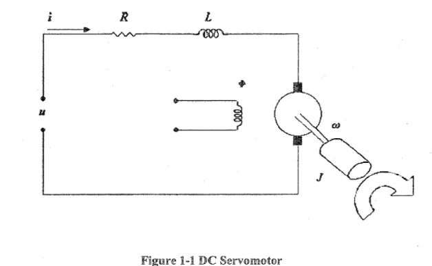
A typical example of multi-time scale system is DG servomotor as shown in Figure 1.1 [29]

U

Figure 1-1 DC Servomotor

DC motor modeling can be separated into electrical and mechanical two subsystems. As we all know, the time constant of electrical system is much smaller then that of the mechanical system. Hence, the electrical subsystem is the fast subsystem.

Kirchhoffs voltage law is used to derive the electrical system: L — = -kco -Ri + u

dt (1.4)

where u is input voltage, i is armature current, R and L are the resistance and inductance

of the armature, K is back EMF constant. The mechanical subsystem follows

d(o

where J is the moment of inertia, k is torque constant of the motor.

Then we apply a transformation of ?G = — ,ir = — , ur = — for ( 1 .4) and (1.5)

J Jk Jk

à)r = ir

: r (1.6)

ar=-ct>r-ir+ur Lk2

where e = —- < 1 , / is the fast state. JR2

b) Parametric Embedding

Unlike the DC motor mentioned above, some system equations only consist of constants with certain values which are measured from experiments. To apply singular

perturbation theorems to these models which do not contain any parameters that can tend to zero or infinity, we need to introduce the small parameters artificially.

We will call a system ? = F{x;s),x e Rd depending on parameters . a one-parametric

embedding of a system.: ? = f(x),x e Rd , if f(x) = F{x,\) for all ? e R" . Similarly, we

can define an ?-parametric embedding, with right-hand sides in the form

f(x) = F{x,\,...,\) and x = F{x\sl,...,sn),xe. Rd . If an ?-parametric embedding has a

form of a fast-slow system with asymptotic structure^,,..., kn), we call it a

(kx,...,kn)-asymptotic embedding.

We use this procedure to replace a small dimensionless constant a with an artificial small parameter ea , where«· «1. The replacement«/ constitutes a one-parametric embedding. There are numerous ways a system can be parametrically embedded, but only the one in which the qualitative features that we are interested in can be best preserved

from the original system is the first choice.

1 .2.5 Identification and control of systems with multi-time scale

The systems which contain fast and slow phenomena can be modeled by singularly

perturbed model. This can decouple the high-order linear or nonlinear system into fast

and slow subsystem that occurs at different moments, which simplifis the complicated dynamic process for numerical study and control design. In [77], a system identification strategy with two time scales is proposed for modeling the Tokamak process based on

experiment data of static plasma response. Then two time-scales reduced-order models

are used to test the optimal control scheme. For some cases, the centralized controller can't stabilize the fast and slow dynamic simultaneously. Then the singular perturbation theory is applied to separate the model into multiply time scale subsystems. Decentralized model predictive controller are developed based on the transfer function matrix of a kind of special systems which is decoupled into two models in different time scales [78]. Comprehensive discussion about singular perturbation and time scales in

control can be found in [79-81].

Neural network are also applied for multi-time scale problem. In [82], a neural controller with two time scales is designed for trajectory tracking of robot manipulator.

Only the fast subnet is learning when the linear parameter is changed, which can save the

computation work. In [83], the flexible-link robot arm system is divided into two time

scales to reduce the spillover effect. The optimal control technique is applied to fast

subsystem, while the fuzzy logic controller guarantees the tracking control performance.

The stability analysis of recurrent neural networks by singular perturbation method is

presented in [28]. In [29], the passivity analysis of the system identification problem

about multi-time scale neural network is developed for further application in control

purpose.

1.3 Research objectives and main contributions of this thesis

Consider a class of nonlinear systems with different time scales. The overall objective of this thesis is to develop on-line identification and control strategies to achieve fast and accurate trajectory tracking performance for such class nonlinear system.

1.3.1 Research objectives

The main research objectives of this thesis are:

1) To develop new updating algorithms and stability analysis for dynamic neural

networks with multi-time scales in the sense of minimizing the identification error for nonlinear systems with or without multi-time scales.

2) To develop NN-based adaptive controller to achieve fast and accurate trajectory-tracking based on the on-line identification results.

L3.2 Main contributions

In this research, system identification and control based on dynamic neural networks with multi-time scales are extensively studied for nonlinear black-box model. The main

contributions are summarized as:

® The Lyapunov function and singularly perturbed techniques are used to develop the on-line update laws for both dynamic neural networks weights and the linear part matrices. The learning algorithm of the linear part matrices is applied to

provide more flexibility and accuracy of nonlinear system identification [84]. • New stability conditions are determined for identification error by means of

Lyapunov-like analysis with new dead-zone indicators which prevent the weights

of neural network from drifting into infinity [86].

« Various control methods are applied for trajectory tracking based on the on-line multiple time scales neural networks identification results for the uncertain

nonlinear dynamic systems [85].

• Simulations have been carried out to verify the effectiveness of these identification and control algorithms.

1.4 Thesis Outline

The thesis is organized as follows:

In Chapter 2, some mathematical preliminaries are introduced along with the

mechanism and structure of dynamic neural network with multi-time scales.

In Chapter 3, the structure of dynamic neural networks with different time scales and the identification algorithm are discussed. Then the adaptive tracking control method and the error analysis are stated followed by simulation results.

In Chapter 4, the improved system identification and control schemes for multi-time

scales neural network are presented.

In Chapter 5, conclusion and some possible future work are given.

1.5 Conclusion

and off-line identification, black-box and grey box and linear and nonlinear identification problem. After a brief discussion about the nonlinear control, we provide extensive literature review on NN-base system identification and control. The basic concept of multi-time scales system is introduced as well. The motivation, research objective and contribution are presented in the thesis.

Chapter 2 Mechanism and Structure of Neural Network

Artificial Neural Networks (ANN), commonly referred to as "neural networks", are mathematical models which are inspired from the structure and functions of the biological neural systems like human brain [1, 2]. Through the massively parallel distributed structure and the ability of learning and generalization, NN are computationally powerful enough to perform some capabilities of the biological neural networks (BNN), such as knowledge storing, information processing, learning and justificafionfl, 3]. As a result, the application areas of NN range from signal processing, patter recognition, data mining, classification, medicine, financial application, to system identification and control.

As mentioned in Chapter 1 , the architectures of neural networks can be categorized into feedforward neural networks and recurrent neural networks (Dynamic Neural Network). In this study, dynamic neural networks are chosen candidates for modeling and control of nonlinear systems with multi-time scales which contain strong noniinearity and uncertainty. The architecture of the recurrent neural networks and corresponding activation functions are introduced in this chapter.

2.1 Feedforward neyra! network

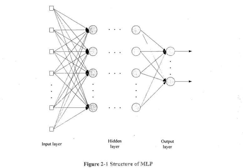
Multilayer feedforward neural network consists of an input layer, at least one hidden layer and an output layer. The general architecture of a multilayer perceptron (MLP) is shown in Figure 2-1 .

Input layer Hidden_laver Output layer Figure 2-Í Structure of MLP

2.2 Dynamic Neural Network

A large class of dynamic systems can be represented in the form of a system of

first-order differential equations written as follows:

x = F(x(t)) -

(2.2)

where F is a vector function, x(t) = [x](t),x2(i)---xy(t)]T

is the vector of the state

variables, ? denotes the derivative of state variables with respect to time t. The vector

function F does not depend explicitly on time t, which makes the system (2.2) to be autonomous. In this paper, we only consider the systems in continuous time domain.

Recurrent neural network distinguishes itself from other neural networks like

feedforward neural network in that it contains at least one feedback loop, which leads to

fact that the neural network can be represented in the form of (2.2). On the other hand,

the neural network, which is in form of dynamic system (2.2), has feedback loops

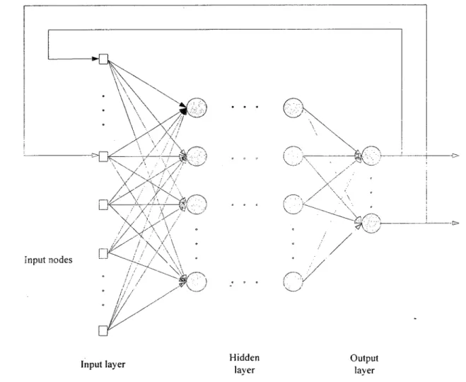
congenitally. As a result, many researchers refer "recurrent" and "dynamic" as the same concept in neural network literature. A common recurrent neural network is show in

Figure 2-2.

Input nodes

Input layer Hidden_laver Output_laver

In this thesis, the architecture of the neural network is based on the following dynamic neural network.

K1=Ax11n +^a(V1X1J + WJ(V2X111MU) (2.3)

where x„„ e R" are state variables of neural networks, Wx eR"xp,W2 e R"*q are the

weight in the output layers, F1 e Rpx" , V2 e Rqx" are the weight matrices describing hidden

layers connection, s^= [s, ([F,x], ,)···s?([^?]??)]G is vector function responsible for

nonlinear state feedback. f e R^ is diagonal matrix:

f = a?a§[f,([?2?\?)-f(?{[???](??)]t . UeR'" is the control input vector and

/(¦):W ->9?" is a differentiable input-output mapping function. A e R"*" is a Hurwitz matrix for the linear part of neural networks.

As we can see that Hopfield-type neural network is the special case of neural network (2.3) with A = diag{a,}, where a¡ = -1/R1-CnR1- > 0 andC,. >0. R1- and C,. are the

resistance and capacitance at the ith node ofthe network respectively.

The three typical activation functions are shown as follows:

1 . Threshold Function. The most common example is illustrated in Fig 2-3.

Í1

if x>0

0.5

-2 -1.5 -1 -0.5 0 0.5 1 1.5 2

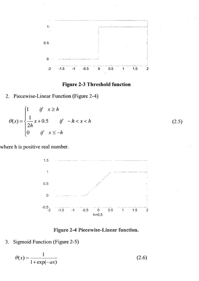
Figure 2-3 Threshold function 2. Piecewise-Linear Function (Figure 2-4)

?{?)

1 if x>h

0 if x<-h

? + 0.5 if -h<x<h

where h is positive real number.

(2.5) 1.5 0.5 -0.5 -2 -1.5 -1 -0.5 0 0.5 1 1.5 2 h=0.5

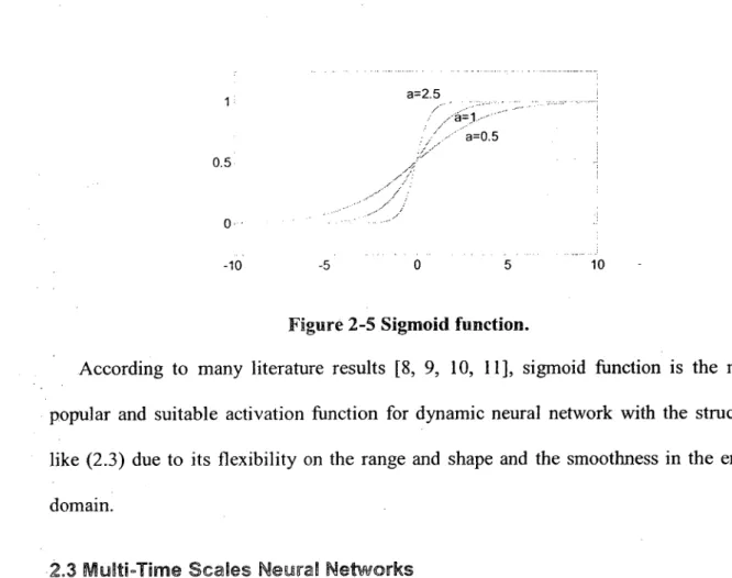
3. Sigmoid Function (Figure 2-5)

1

9{x) =

0.5

0

-10 -5 0 5 10

-Figure 2-5 Sigmoid function.

According to many literature results [8, 9, 10, 11], sigmoid function is the most popular and suitable activation function for dynamic neural network with the structure like (2.3) due to its flexibility on the range and shape and the smoothness in the entire

domain.

2.3 Multi-Time Scales Neural Networks

A wide class of nonlinear physical systems contains slow and fast dynamic processes

that occur at different moments. In order to identify and control this kind of system we

will utilize the Dynamic Multi-Time Scales Neural Networks (DMTSNN) as the modeling tool, which is inspired from neural network (2.3) with the perturbation

parameter embedded.

K„ = Ax111, + W,ax (F1 [x, >f) + W2^ (F3[x, y]T)U

^ ?)

4>„„ = Bym + W3a2(V2[x,y]T) + WJ2(V4[X, yf )U,

where xm e R", ynn e Rn are the slow and fast state variables of neural networks,

xtR", y e R" are the state variables of the real system. W12 e R"x2" , Wi4eR"x2n are the

weights in the output layers, F1 2 e R2"*2" ,F34 e R2""2" are the weights in the hidden layer

a=2.5

s? = [s? (?, ) · - · (Tk (?p ), s? (?, ) · · · s? ( ?„ )f eR2" (£ = 1,2),

are diagonal

matrices,

fk=?ag[fl2(xì)¦¦¦f]2(xl),f]2(yJ¦¦¦f¡2(yJ]teR2"^

e /?2" is the control input vector, A e R"*" anàB e R"*" are the unknown matrices for the linear part of neural networks, the parameter e is a unknown small positive number. When e is equal to 1, the neural network (2.7) becomes a normal one [12]. The typical presentations of the activation functions s? and ^kare sigmoid functions.

In order to simplify the theory analysis, we make the hidden layer weight V to be an

identity matrix, which makes DMTSNN (2.7) become a single layer neural network.

*m = Axu„ + Wx s, (?, y) + W2 f, (?, y)U %„ = By„„ + p?s? (?> y) + wi<f>2 (*, y)u

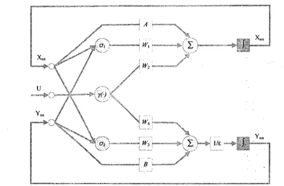
The structure of the DMTSNN (2.8) is shown in Figure 2.6

(2.8) A U™ Q-j l.,,,:,rS„„„„:Jp[ ?] .„.:, „,«..,.,„I^^ï x„„ 1 \v //¦ ? / \ \ ^ -> — ^, \ V: -.,;¦'¦ : ?2 'I, Yn A'' SA B

We apply the activation function ak and f? in DMTSNN (2.8) as the following

types:

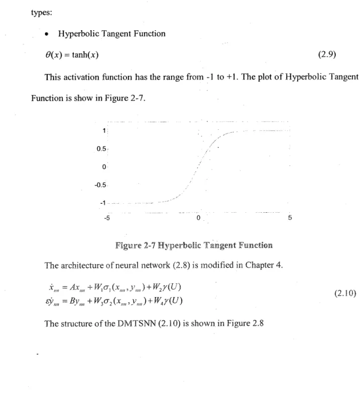
• Hyperbolic Tangent Function

?(?) = tanh(jc) (2.9)

This activation function has the range from -1 to +1. The plot of Hyperbolic Tangent Function is show in Figure 2-7.

1j ' ; ^.

-0.5:

/

Figure 2-7 Hyperbolic Tangent Ftinction The architecture of neural network (2.8) is modified in Chapter 4.

Kn =Ax„„+Wlai(x,„„ylJ + W2r(U) ?,,,, = By,,,, + W1G1 (X111, , ynll ) + w4r(U)

Figure 2-8 Structure of modified dynamic neural network with two time-scales The activation functions defined in (2.4), (2.5), (2.6) and (2.9) range from 0 to +1 . For the neural networks in Figure 2.8, we use the Logistic Function with multi-parameters (Figure 2-9). which can range differently and widely.

<? Logistic Function with multi-parameters.

?(?) a 1 + exp(-èv) — c (2.11) 1.5 1 0.5 -0.5 -10 0 a=1, b=1, c=0.5 10

2.4 Conclusion

In this chapter, the mechanism and structure and the main definitions of the dynamic neural networks are introduced. An important mathematical preliminary is given for the

further study. The basic mechanism and structure of DMTSNN used in system identification and control are given.

Chapter 3 Identification and Control for nonlinear systems with

multi-time scales

Traditional linear control methods cannot deal with the nonlinear systems with incomplete or none information of dynamics. A common approach to deal with these problems is to utilize proper modeling and identification techniques in the control scheme. In this chapter, a dynamic neural network model is proposed for nonlinear system with multi-time scales and on-line identification algorithm is developed for its parameters so that the output of the model approaches to the output of the actual plant. By using the Lyapunov method and singularly perturbed techniques, an adaptive controller is designed based on the neural network model to control the states of nonlinear system to track reference trajectories.

3 J On-lin® identification

A large number of strategies have been proposed for the identification of dynamic systems with highly nonlinearities and uncertainties. Dynamic neural networks have been

applied in system identification for those systems for many years. Due to the fast

adaptation and superb learning capability, they have transcendent advantages compared to the traditional methods [14], [1 5].

3.1.1 WonSinear systems with multi-time scale

Numerous systems in the industrial fields demonstrate nonlinearities and uncertainties which can be considered as partial or total black-box. A wide class of nonlinear physical

section we consider the problem of identifying this class of singular perturbation nonlinear systems with two different time scales described by

x = fx(x>y>u>t)

(3 n

*y = fy{.x,y,u,t),

where ? e Rp and y ei?' are slow and fast state variables which are totally measureable, the functions fx and f are partially or totally unknown but continuously differentiable, UeR' is the control input vector and e > 0 is a small parameter.

3.1.2 Dynamic NN model

In order to identify the nonlinear dynamical system (3.1), we employ the dynamical

neural networks (2.8) with two time-scales:

*«„ = Axnn + Wp1 (x,y) + W^ (x,y)U

As we mentioned in Chapter 2 the slow and fast state variables of the DMTSNN are

x„n e R",y„„ e Rn . Wi2e i?"x2"5 W^ 4 e i?"x2" are the weights in the output layers. We use

the state variables of the neural network to identify the object dynamic model respectively, where ? = max < p.q > ¦

Generally speaking, when the dynamic neural network (2.8) does not match the given nonlinear system (3.1) exactly, the nonlinear system can be represented as

where W* , W2 , W* , W4 are unknown nominal constant matrices, the vector functions

Afx, AfY can be regarded as modeling error and disturbances, and A* , B* are the

unknown nominal constant Hurwitz matrices.

Remark 3.1 : In literature of system identification and control based on neural network like (2.3) or (2.7) [8 - 11], the authors coherently make a strong assumption that the linear

part matrices A and B were posed as known Hurwitz matrices and such assumption is

sometimes unrealistic for the black-box nonlinear system identification. Here we apply the on-line identification process to the linear part matrices dynamic to approximate to their nominal values.

It is assumed that the states in system (3.1) are completely measurable. And the number of the state variables of the plant is equal to that of the neural networks (2.8). The identification errors are defined by

Ar = ? — ?

(3.3) ày = y-yn„.

From (2.8) and (3.2), we can obtain the error dynamics equations

Ar = A*Ax + Ax1111 + Wxa,{x,y) + W^{x,y)U + Afx

eAy = B Ay + By1111 + W2a2 (x, y) + W4<f>2 (?, y)U + Afy ,

where W1=W* - W1 , W2=W2* - W2 , WZ=W¡ - W, , W4=W4' - W4 and A = A* - A, B = B* - B .

3.1.3 Adaptive identification Algorithm

The Lyapunov synthesis method is used to derive the stable adaptive laws. Consider

v,=vx+vv

Vx = Ax7PxAx + îr{w7PxWx }+ tr{w¡ PxW2 }+ ??{a ? Pxa}

(3.5)

?? = AyTPvAy + tr{w¡PvW3 }+ tr{w4TPyW4 }+ tr{ßTPyß}.

Since the matrices A* , B* are unknown nominal constant Hurwitz matrices, there definitely exist matrices Px, P1. which can be chosen to satisfy the following equations, where Qx , Qx are positive definite symmetric matrices:

(3.6)

A7Px^PxA = -Qx

B*TPy+PvB*=-Qy.

Hence, differentiating (3.5) and using (3.4) yield

Vx = -Ax7QxAx + 2Ax7PAx11n + 2Ax7PxW^ (x, y) + 2Ax7PxW2f? (x, y)U

+ 2Ax7PJx + 2tr\ATPxA]+ 2tr\W7PxW, }+ 2tr\w¡PxW2 } ,

Vv=-(l/s)Ay7QyAy + {l/e)2AyTPvBym + {?/e)2??7?ß:s2(?,?)

(3'7)

+ (;i/s)2AyrPrWJ2(x,y)U + {\/s)2AyTPJy + 2tr)BT'PrBj

+ 2tr^7pß3\+2tr\Wf?ß4\ ,

Theorem 3.1: Consider the identification model (3.2) for (3.1). If the modeling error

and disturbances are assumed Afx = 0, Afv=0, the updating laws

À = Axx7m

B = (\/s)Ayyl

W1 = ??s[ (x, y)

W3 = {\/s)Aya7 (x, y)

(3 . 8)

W2 = Axu7f7 (?, y)

W4 = '\/s)Ayu tf[ (?, y),

can guarantee the following stability properties:

2) HmAx = O, HmAy = O and lim ^. = 0,/ = 1,···4.

Proof: Since the neural network's weights are adjusted as (3.8) and the derivatives of the neural network weights and matrices satisfy the following WL2JA = WL2_3A, A = A,

B = B from (3.7), Vx.,Vx become

Vx =-AxTQxAx + 2AxTPxAfx

Vx = -{\/e)AyTQyAy + (l/e)lAyTPxAfx

If fx = 0 , fx = 0 , then one obtains

? = HMIo, ^ ? .'? = -0/F4,. - °

K = Vx + ?, < O

where Vx , Vy are positive definite functions and Vx, Vx < O can be achieved by using the

updating laws (3.8) when Afx =0, Afy=0 which implies Ax,Ay,Wì23A,A,B e Lx .

Furthermore, ? =Ax +?. ? , =??+? are also bounded. From the error equations (3.4)," ¡lit ' *¦ 111! ·* -" x v ¦*

we can draw the conclusion that Ax, Av e Lx . Since Vx , Vr are non-increasing function

of the time and bounded from below, the limits of Vx, Vx (HmKx,. = Kvv(co)) exist.

Therefore by integrating Vx , Vy on both sides from 0 to co, we have

G||??|? = [Kv(0)-KT(oo)]<co

*

a

'

(3.10)

The above inequalities imply that ??, Ay e L2 . Since ??, Ay e L2 ? Lx and

??,?? e Lx , using Barbalafs Lemma[13] we have HmAx = O5HmAy = 0. Given that the

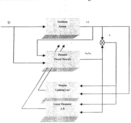
control input U and s, 2(')>F\ 2(') are bounded, it is concluded that HmPP12 =0, HmPf3 4=0. The identification scheme is illustrated in Figure 3.1 .

Nonlinear System ,,'"?"'*.- fi^K' *$&

//

a

Figure 3-1 Identification scheme

Remark 3.2: When e is very close to zero, both W3 and W4 exhibit a high-gain behavior, causing the instability of identification algorithm. The Lyapunov function (6)

can be multiplied by any positive constant a, i.e., B~r(aPy) + (aPr)B~ =-aQy, the

adaptation gains of W3 and W4 become (]/e)a?? , which turn into small gains if a is

Corollary 3.1: For the dynamics of error system equations (3.4), if we define fx , f. as the inputs, the update laws (3.8) can make (3.4) input-to-state stability (ISS) with the assumption that there exist positive definite matrixes ? t , ?? such that

KJQ^KJPAAi

KJQy)iKJPA>p>y

2Ax7PxAfx < Ax7PxAxPxAx+AfJAjAfx

{\¡e)2AyTPyAfy < {\/e)??t??A rPyAy + (l/S)AfJA^Afy

Then equation (3.9) can be represented as

(3.11) Proof: Using the following matrix inequality:

X7Y + [X7Y)7 < X7A^X + Y7AY

(3.12)

where X,YeRjxk are any matrices, ? e RJ*k is any positive definite matrix.

We obtain

(3.13)

Vx = -Ax7QxAx + 2Ax7PxAfx

< -KJQAMf + Ax7PxAxPxAx + AfJAjAfx

(3.14)

<-ax(\\Ax¡) + flx(\\Afx¡)

V2 = -{ì/e)AyTQvAy + (l/'e)2Ay7PvAf

* -(V^Kni„(ö,-)||A>i|2 + {?/e)??G??? , PxAy + {?/e)AfJAjAfy

(3. 1 5)

<-ay{\Ay\) + ßy{\Af\)

where

«, (¡??||) = µ„„„ (Q, ) - Kn (^??))|??2 > A (?????) = ?» (*;' )\? If

We can select a positive matrix Ax and A1. such that (3.11) is established. Since

ax, ßx, a?, ßy are Kx function, Vx, Vv are ISS-Lyapunov function. Using Theorem 1

in [16], the dynamics of the identification error (3.4) is input to state stability.

Theorem 3.2: If the model errors Afx , Af. , are bounded, then the updating law (3.8)

can make the identification procedure stable [8]: Ax,AyeLx WÌ234,A,B e Lx

4,BeLx.

Proof: The input to state stability means the behavior of neural network identification

should remain bounded when its inputs are bounded [16]. 3.1.4 Simulation Results of identification

To illustrate the theoretical results, we give the following two examples.

Example 1 : Let us consider the nonlinear system

X1 = GT1X.+ P1SIgTl(X2) + U1

Sx1 - Ct2X2 + ß2sign(xx ) + U1 ,

where we use the same parameter a, = -5 , Qr2 =-10, ß, =3, ß2=2, X1(O) = -5.

X2(O) = -5 . The given nonlinear system, even simple, is interesting enough, since it has

multiple isolated equilibriums [9]. Using the parameter embedding technique [12], the model used here is singularly perturbed and the small parameter e is positive and smaller than 1. The input signals are selected as: U1 is a sinusoidal wave (w, = 8sin(0.05i)) and

u2 is a saw-tooth function with the amplitude 8 and frequency 0.02Hertz.

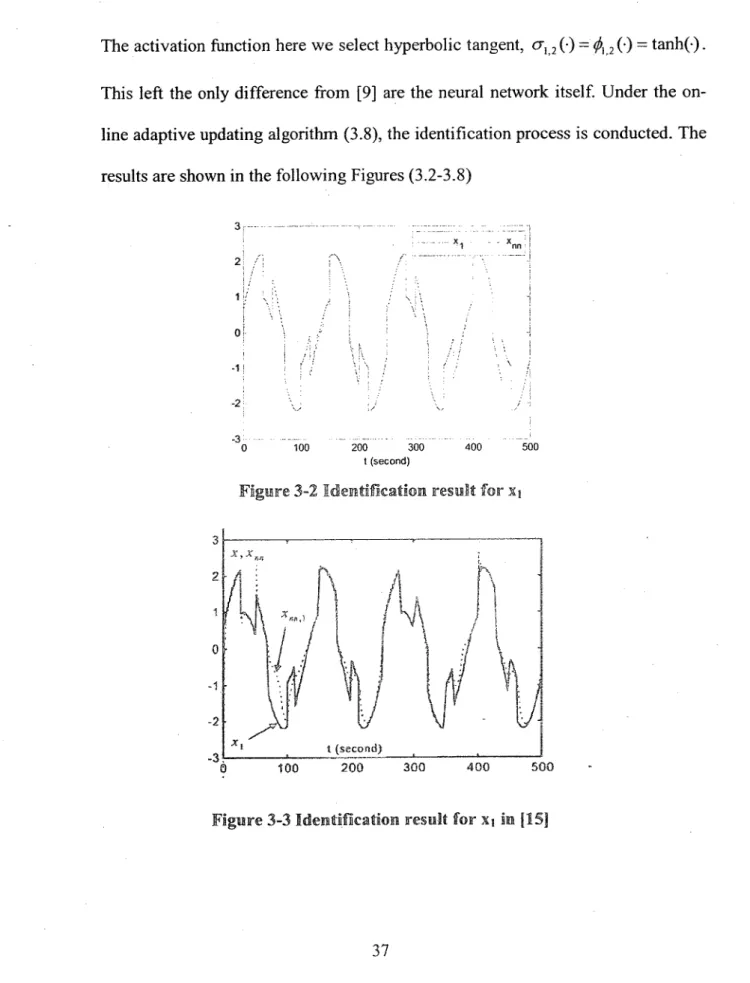
The activation function here we select hyperbolic tangent, s? 2(·) = f? 2(·) = tanh(-). This left the only difference from [9] are the neural network itself. Under the on-line adaptive updating algorithm (3.8), the identification process is conducted. The

results are shown in the following Figures (3.2-3.8)

2Ì ?. ?? ?: "

:?"~-100 200 300

t (second)

400 500

Figure 3-2 Idemtifieation result for xj

t (second)

100 500

??

-3

100 200 300

t (second)

400 500

Figure 3-4 Identification error for ?]

3, X2 Vnn ^1 ? -3 100 200 300 t (second) 400 500

?..r -1 -2

X-\

IXN

Figure 3-6 Identification result for X2 in [IS]

Ay

-2

100 200 300

t (second)

400 500

Ta: Yb

-10 -¦

0 100 200 300 400 500

Figure 3-8 The eigenvalues of the linear parameter matrices

To show the identification performance of the proposed algorithm, the performance index -Root Mean Square (RMS) for the states error has been adopted for the purpose of

comparison.

RMS = J Ze2O') ?

;=i

where ? is number of the simulation steps, e(i) is the difference between the state

variables in model and system at i'h step. For state variable x,, the RMS value is

0.232782 and RMS for state variable x2 is 0.149096.

The results in Figures 3.2-3.8 demonstrate that the identification performance has been improved compared to those in [15]. It can be seen that the state variables of dynamic

multi-time scale NN follow those of the nonlinear system more accurately and quickly.

for both A and B are universally smaller than zero, which means they are always stable

matrices.

b) Now we consider model (3.16) with multi-time scales. The small parameter e is selected as 0.2. The sigmoid functions are chosen as

(3.17) 1 + exp(—ox)

The parameters for each sigmoid function in dynamic neural networks are listed in

Table 3-1.

Table 3-1 Sigmoid function parameters

s,(?,?) 2 2 0.5

f,(?,?)

(?2

02

??G

s2(?,?)

2

2

05~

f,(?,?)

02

02

^??

The results are shown in the following Figures (3.9-3.14).

-3

?? i -3 100 200 300 t (second) 400 500 -2

Figure 3-10 Identification error for Xj

*2

100 200 300 400 500

3--

-

-3-O 100 200 300

t (second)

400 500

•ïgure 3-12 Identification error for ?2

-2 -3--4 -5 -6 100 200 300 t (second) 400 500

2! O*" W₁₁ W 12 0 100 200 300 400 500 1; -2 -3 W 22 -.' ¿ 'y' .-. \'' W₂₁ 0 100 200 300 400 500 b)W9 1 r

0.5 I

Figure 3-14 The learning process of the updating weight matrices

For state, variable Xi, the RMS value is 0.139102 and RMS for state variable X2 is 0.1 16635. The results in Figures 3.9-3.14 demonstrate that the state variables of dynamic multi-time scale NN follow those of the nonlinear system accurately and quickly. The

eigenvalues of the linear parameter matrices are shown in Figure 3.13 The eigenvalues

for both A and B are universally smaller than zero, which means they are kept as stable

during the identification. Figure 3.14 shows the learning process of the updating weight

matrices of the dynamic NNs.

Example 2: In 1952, Hodgkin & Huxley proposed a system of differential equations describing the flow of electric current through a surface membrane of a giant nerve fibre. Later this Hodgkin-Huxley (HH) model of the squid giant axon became one of the most

important models in computational neuroscience and a prototype of a large family of mathematical models quantitatively describing electrophysiology of various living cells

and tissues[12][17].

^L = J_(Iext-gKn^V + En.-EK)-gNamih(V + En-ENa)

-gl(V + EH,-E,)) dn _ nx - ?

dt~ Tn

where time t is measured in ms, variable V is the membrane potential in mV, and n, m and h are dimensionless gating variables corresponding to K+, Na+ and leakage current channels respectively, which can vary between [O5I].

ccn a,„ T a,,

n„ = — m„ = ¦

Otn + ß„

°°

GC1n + ßm

*

a,, + ß„

1 1 . 1

t,. =¦

"

a,+ß„

'"

am+ßm

"

ah+ßh

0.01(10- V) 0.1(25-F) -L

a„ = —w=i

am = — «=E

a» = ome 2°

e io -1

e io -1

^

j

_V_

V_

ßI, - 30-G

ßn =?.?25ß"80

ßm=Aex%

e'w + l

gK = 36mS I cm g Na - 1 207775 / cm g, - 0.3mS I cm EK =-l2mv ENa =U5mv E1 =10.599/wv CM = IpF /cm'

From the electrophysiology point of view, the most important state of the HH system is the membrane potential V which has multifarious electro-physic phenomena and is also

the core of the numerous former researches.

Instead of using the original HH model, we use the (2, 2) asymptotic embedded system [12]. We take the modified HH model with the effect of extremely low frequency (ELF) external electric field En. which serves as the other control input besides the external applied stimulation current Ie:l .

Since numerous researches have been carried out on applying various stimulations to HH model, whether the states of NN can still follow those of the HH system with these

different stimulations becomes our first priority. So some classic inputs are applied to the

system.

Iext = \A, (cosœ,t + Y)

2 !

'

(3.19)

Ei%. = \AE cos coEt

where ?, E = 2nf¡ E , and all the initial conditions for the HH system are the equilibrium (quiescent). V0 = 0.00002 , m0 = 0.05293 , A0 = 0.59612 , n0 = 0.3 1768 .

We pick two typical stimulations which can result in significant and classic neuron

excitation:

150 ^ 100 E 50 > Oy -50 0 100 200 300 400 500 150 ? 100

è

50

c 0.5-V--V; ..\^;^'?? ;-??^·-'^ V*vvvVw^ fyvVVV^V^ Í^V^i

Figure 3-15 Identification results

In the plot for state V, n, m, h, the real lines are the real state variables for the HH system and the dot lines represent the identification state in the NN. The second plot is the

O-·; ->... ^.-'-??1. ^. ^.??2 _2 · :.';'?-:¦· ¦ - ¦ · - :·? :^'??2_.^ -4 ¦ - ¦ - - ... O 100 200 300 400 500 0; :-. . ? ¦ :· . -20 X'' · ?''-?. -' . -??^;:'- V-.. '--··. -..../ ?"·'"--'---';-· -40 '¦ ¦ ~ - -^- ??1 0 100 200 300 400 500 time (ms)

Figure 3-16 Eigenvalues of the linear matrices A, B

0,AE= \0mV , fE = 1 \5Hz , e = 0.2 . 150 100 50 O- ·-.-- --..-- - - -'.-·-¦ .'.-¦¦¦¦ --.. -.,--¦ -50 0 100 200 300 400 500 150 100 50 0 . . -50 0 100 200 30G 400 500 1 ¦ - -0.5 '. -, -, 0 . . 0 100 200 300 400 500 1.5 1 0.5 0 - ¦"'- - ¦ --- - · ¦- ¦ --- - - .-.-.- . . ¦-.- -. -¦ -0.5 . . .. . 0 100 200 300 400 500 1 . . ...

o.s^'v^ 7/"""' 'V-''''V"·" >'"" '.""' '"·.-¦¦"'' '¦¦·¦'"' 'V"'" \-""'

In the plot for state V, n, m, h, the real lines are the real state variables for the HH system and the dot lines represent the identification state in the NN. The second plot is the

identification error for the membrane potential.

o:..-.„. ^"V1 -2 ., . . :< ??2 ??2 _4 L 0 100 200 300 400 500

. O^ ^

Figure 3-18 Eigenvalues of the linear matrices A, B

In simulation a), System is in 8/1 phase locked oscillation periodic bursting. RMS value of the state variables are RMSn=0.074642, RMSh=0.083497, RMSV=0.438275,

RMS1n=O.035473. In b), System is in same frequency periodic spiking. RMS value of the

state variables are RMSn=0.05695, RMSh=0.061458, RMSV=0.86327, RMSm=0.060288.

The time scale is considered by putting e = 0.2. From Figures 3.15-3.18, we can see that

the states of NN model can follow those of HH model very closely. The identifi

cation-performance of the proposed algorithm is very good, especially for the membrane potential. The eigenvalues of A and B for a) and b) converge to the same steady values since the nominal linear matrices Ä and B* do not change with different inputs.

3.2 NN-foased adaptive control design

Traditional nonlinear control techniques have been developed and applied for many decades, but they are not efficient when facing the plants with incomplete information.

The past decade has witnessed great activities in neural networks based control for the

models with nonlinearity and uncertainty. The tracking problem is investigated based on

the identification results from Section 3.1.

3.2.1 Tracking error analysis ¦

From section 3.1 we know the nonlinear system may be modeled by dynamic neural

networks with the updating laws (3.8):

? = Ax + WxOx (x, y) + W1(J)x (x, y)U + Afx

ay = By + Wzo2 (x, v) + W4fa (x,y)U + ?/? ,

(3'20)

where the model error and disturbances Afx , Af. , are still assumed to be constrained as before. And also Wi234 are bounded as well as other stability properties in Section 3.1 .

The model error in most cases could be zero or negligible, however, even if the dynamic neural networks have superb learning ability to represent the nonlinear dynamic process, the model error are sometimes inevitable or even may affect the stability of the system. The following controller design considers this model error for more general

situations.

Hence, the control goal is to force the system states to track the desired signals, which

are generated by a nonlinear reference model

The overall structure of the neural networks identification and controller is shown in Figure 3.19. ;' Referracé'.;-HÜ Nontmear System Dynamic Neural Network *d.yd x>y Weights Updating Law .Control ; ^??,?? Linea- Parameter ^S-Ec 0

Figure 3-19 identification and control scheme

We define the state tracking error as Ex =x-xd

Er =y-yd- (3.22)

Then the error dynamic equations become:

Ex = Ax + Wpx (x, y) + W2<f>x (x, y)U + Afx - gx

Then the control action U is designed as

U = uL +uf, (3.24)

where uL is a compensation for the known nonlinearity and uf are dedicated to deal with

the model errors, which can be left open if it is zero or ignorable. Let uL be

U, = U1 = \¥2f?(?, y)

{\/e)WJ2(x,y)

(Vs)By1

(ì/e)W3a2(x,y)

The control action uf is to compensate the unknown dynamic modeling error. The

sliding mode control methodology is applied to accomplish the task. So let uf be,

"/ = WMx,y)

(i/S)Wj2(^y).

Uj- = ¦ AEx -kx sgi{Ex)

¦ (?/e)??? - (l/e)ky sgn(£,.

fhe modeling error and disturbances are assumed to be bounded. Hence we have

?/?|<??,?/?<??:

Theorem 33: Consider nonlinear system- (3.1) and the identification model (3.2).

With the updating laws (3.8) and control strategy (3.24), we can guarantee the following

stability properties:

1) Ax7AyJV1 23A, A, B e Lx and Ax,Ay^L2

3) lim£r =0,lim£y =0

Proof : If we consider the identification and control as a whole process, then we can

apply the strategy to real applications by generating the final Lyapunov function

candidate as V = V1 + Vc .

In section 3.1 , we had already proved V1 < 0 and the stability properties in Theorem 3.1. Now let's consider the Lyapunov function candidate for control purpose

V.=ElEr+ElE„.X X V V (3.29) First rewrites (3.23) as Ex È. Ax

(Ve)By

{y£yv3a2(x,y)

{\/e)p?f2(?,?)_

(V*Wr

(Ve)gv

Then substituting (3.25) into (3.30) obtains Ex E . AEx

(\/e)???

'WJ1(X, y)

[

(l/s)fVJ2(x,y)jUr +

(VeWr

If the model error and disturbances are zero or negligible which, from the control

point of view, means it won't devastate the stability of the system, uf can be chosen to

be zero which will lead the error dynamics converge to the origin. Proof is quite straightforward since A and B are stable matrices and e is positive.

Then substituting (3.26) into (3.31) yields

Èx=AEx + u'fa+àfx

Èy=(ì/e)BEy+t/fi + (Ve)Afy.

By using (3.32) and (3.27), we obtain the derivative of (3.29) as

Vc = 2ETxÈx + 2ETyËv

= 2ETx(AEx+u'fa +fx) + 2ETy({l/e)BEy +u'& +(l/s)Afy)

= -2kx\Ex\\ + 2Elfx -2{lle)ky\\Ey\\ + 2{l/s)àcyTAfy

<-2*,|£j + 2l^|ArJ-2(l/ff)fcf||£rI + 2(l/^j4rJ

.

=-2(^-||??||)||^||-2(?/^?^-||?/?||)||£?||

If we choose Icx > àfx,ky > ?/\, , then Vc <0. Hence, we have stability properties 3)

lim£v=0,lim£v=0,and V = V1 +Vc<0._{I—>cc /—>co}

With consideration of the modeling error and disturbances, the sliding mode control logic (3.27) can guarantee the tracking stability without the assumption that A and B are

stable matrices.

The controller involves matrix inversion which can guarantee the non-singularities by

choosing the proper initial values of the parameters in the updating law and the activation

function.

3.2,2 Simulation results of control scheme

We continue the process in Section 3.1 for nonlinear system (3.16). instead of using input signals sinusoidal wave and saw-tooth function, we implement the control law to obtain the control signal to the nonlinear system (3.24). It constitutes a feedback linearization and a sliding mode compensator. The desired trajectories are generated by

the reference model

X" = y"

(3.33)

xd ?

10 20 30 40 50

t (second)

Figure 3-20 Trajectory tracking of ?

20 30

t (second)

Figure 3-21 Trajectory tracking of y

The time scale is considered by putting e = 0.2. From Figures 3.20 and 3.21, we can

see that the states of the nonlinear system can track the desired trajectories in 20 seconds. For state variable x, the RMS value is 0.5246 and RMS for state variable y is 1.64141 1

Since the small parameter accelerate the state y, it takes relative more time for the state of the system ? to track the reference signal. The simulation results demonstrate that the

proposed identification and control algorithm can guarantee the tracking performance of

nonlinear and uncertain dynamic systems. 3.3 Conclusion

In this chapter we propose a new on-line dynamic multi-time scale neural networks identification algorithm for both dynamic neural networks weights and the linear part matrices for nonlinear systems with multi-time scales. The proposed algorithms are applied to identify a second order nonlinear system with multiple equilibriums and the

famous well-studied HH model which has complicated and multifarious system

performance when different inputs applied. Both identification results show the

effectiveness of the proposed identification algorithms.

Furthermore, we propose an adaptive control method b