Array Signal Processing for Synthetic Aperture Radar (SAR)

(1)

ARRAY SIGNAL PROCESSING FOR

SYNTHETIC APERTURE RADAR (SAR)

THESIS

BY

QIFENG LIU

DECEMBER 2018

(2)

Array Signal Processing for

Synthetic Aperture Radar(SAR)

by

Qifeng Liu

B.Eng

A master thesis submitted in partial fulfilment

of the requirements for the award of

Master of Philosophy

Supervisors:

Dr. Wei Liu

and

Dr. Xiaoli Chu

December 2018

(3)

c

(4)

At this moment, I would like to express my sincere gratitude to my supervisor, Dr. Wei Liu, for the support and help of my study and related research.

Furthermore, I wish to present my special thanks to my parents for their love, support and encouragement.

(5)

Abstract

Synthetic aperture radar (SAR) is a kind of imaging radar that can produce high resolution images of targets and terrain on the ground. At present, most of SAR processing algorithms are based on matched filtering. This method is easy to implement and can produce stable results. However, It also has some limitations. This approach must obey the Nyquist sampling theorem and the resolution depends on bandwidth of pulses. This means that the matched filter approach must be based on a large amount of raw data but the performance is limited. With the development of radar imaging, it is difficult for the matched filtering approach to meet the requirement of high resolution SAR iamges.

In this thesis, a new processing method based on the least squares (LS) beamforming is utilized in the processing of SAR raw data. The model of SAR simulates an virtual linear array. The processing of SAR data can also be seen as a process of beamforming. The 1-D azimuth direction echo data is processed using the beamforming method. Simulation results based on the least squares design method are compared with the matched filtering method and the conventional beamforming method with different windows.

(6)

List of Figures

2.1 Concept of aperture synthesis. . . 9

2.2 Train of transmitted and received pulse. . . 11

2.3 SAR data acquisition geometric model. . . 13

2.4 LFM signal waveform. . . 16

2.5 Output signal after pulse compression. . . 17

2.6 Elevation beam width in elevation plane. . . 18

2.7 Side-looking model SAR geometry. . . 20

3.1 Block diagram of range-Doppler algorithm. . . 34

3.2 Signal diagram after range compression [1]. . . 36

3.3 Signal diagram after the RCMC [1]. . . 39

3.4 Signal diagram after the azimuth compression [1]. . . . 41

3.5 Intensity of the point target. . . 43

3.6 Impulse response (point target result) in the range di-rection. . . 45

3.7 Impulse response (point target result) in the azimuth direction. . . 45

3.8 Input image of the area target [49]. . . 48

(10)

3.10 A general co-prime array structure. . . 51 3.11 Structure of the CopSAR concept. . . 52 3.12 Intensity of point target processed by the CopSAR. . . 55 3.13 Impulse response (point target result) of s1(x, r) in the

azimuth direction. . . 57 3.14 Impulse response (point target result) of s2(x, r) in the

azimuth direction. . . 57 3.15 Impulse response (point target result) of s12(x, r) in the

azimuth direction. . . 58 3.16 Impulse response (point target result) of the

conven-tional SAR in the azimuth direction. . . 58 3.17 Intensity of ship target processed by the CopSAR. . . . 60 3.18 Intensity of ship target processed by the conventional

SAR. . . 60 4.1 Matched filter method (range-Doppler algorithm). . . . 64 4.2 General matrix pattern of SAR raw data. . . 67 4.3 Conventional beamforming with rectangular window. . 72 4.4 Conventional beamforming with Hanning window. . . . 73 4.5 Conventional beamforming with Hamming window. . . 74 4.6 Conventional beamforming with Blackman window. . . 75 4.7 Conventional beamforming with Kaiser window(β=2.5). 76 4.8 Beam response of beamformer based on the least squares. 81 4.9 Steps of SAR processing based on the least squares

(11)

4.10 SAR processing method based on the least squares beam-forming for ∆s=50m. . . 86

(12)

List of Abbreviations

SAR Synthetic Aperture Radar

ULA Uniform Linear Array

DoA Direction of Arrival

SNR Signal-to-Noise Ratio

TBP Time-Bandwidth Product

LFM Linear Frequency Modulated

NFLM Non-Linear Frequency Modulated

RCM Range Cell Migration

RCMC Range Cell Migration Correction

SRC Secondary Range Compression

ECS Extended Chirp Scaling

NCS Non-linear Chirp Scaling

FS Frequency Scaling

CopSAR Co-prime Array SAR

(13)

CS Compressed Sensing

NP-hardness Non-deterministic Polynomial-time Hardness

BP Basis Pursuit

MP Matching Pursuit

OMP Orthogonal Matching Pursuit

FFT Fast Fourier Transform

IFFT Inverse Fast Fourier Transform

PSLR Peak Side Lobe Ratio

IRW Impulse Response Width

(14)

Chapter 1

Introduction

1.1

Research Background

In the past 30 years, synthetic aperture radar (SAR) has been widely applied in a multitude of application fields, such as the geoscience re-search, the climate change rere-search, the monitoring of Earth system and environment and even planetary exploration [30]. SAR can be utilized in the area of earthquake disaster monitoring [37] and map-ping global surface of other planets, such as Venus, which has a thick atmosphere [41]. SAR can be considered as an active microwave re-mote sensing instrument. It transmits electromagnetic waves sequen-tially, collects echoes reflected from ground targets and stores data in order to process focused images. Compared with optical imaging sys-tems, SAR can provide high resolution images without consideration of daylight, cloud coverage and weather conditions. This is particu-larly significant in some high latitude areas (polar night) and in some bad weather conditions [11].

(15)

Imaging techniques always desire higher resolution so that we can obtain more details and information from images. SAR is an airborne or spaceborne imaging radar which utilizes the moving of platform to synthesize an antenna with a large aperture. This is why it is called synthetic aperture radar. SAR works in a similar way as a phased array and can be considered as a uniform linear array. The only dif-ference with a phased array with many parallel antennas is that SAR uses only one antenna in time-multiplex. With the moving of the an-tenna platform, the anan-tenna transmits pulses and collects echoes from different ground targets at different geometric positions and creates an virtual uniform linear array (ULA). Because an virtual ULA is cre-ated by SAR, the process of imaging can be trecre-ated as array signal processing and we can use methods of array signal processing to obtain focused images. This is why we are expecting to use the beamforming method to acquire a focused image in SAR.

Array signal processing can be divided into two main areas: beam-forming [52] [23] and direction of arrival (DoA) estimation [6]. Beam-forming, which is also called spatial filtering, is a signal processing technique to form a directional beam for signal transmission and re-ception [52]. This technique can be achieved by combining elements in different sensors or antennas of an array. Compared with temporal filtering, spatial filtering (beamforming) can separate desired signal from interference even if they occupy the same temporal frequency band [52]. A directional beam, which points to the desired signal, is

(16)

formed so that we can collect the desired signal and suppress interfer-ence signals. In array signal processing, DoA estimation is another key research field to estimate the direction angle of impinging signals by an antenna array. The DoA estimation has two main research aspects: self-adaption array signal processing and spatial spectrum estimation. These two aspects have developed rapidly adn are still being devel-oped [31].

In the past decades, most of processing algorithms of SAR are based on the matched filter method, such as the range-Doppler al-gorithm [5] [26], the chirp-scaling alal-gorithm [44] and the ω −k algo-rithm [3]. These algoalgo-rithms convolve the raw data with matched fil-ter reference functions in order to compensate for the phase difference and maximize the value of SNR. However, with the increasing require-ment of resolution, the limitations and disadvantages of this method become apparent. For instance, the challenge for hardware due to high sampling rate, high computation, and large on-board memories and downlink throughput. Also, the image resolution obtained by the matched filter method is limited because of the width of mainlobe and the sidelobe effect.

1.2

Research Aims and Objectives

Currently, most of SAR processing methods are based on matched filter. However, the methods based on matched filter have many

(17)

dis-advantages and limitations. Firstly, matched filter must obey the Nyquist sampling theorem. The sampling frequency must be larger than the signal bandwidth in order to avoid the distortion. The reso-lution is related to the signal bandwidth. This means that higher res-olution requirement will result in a higher sampling frequency. Large amount of raw data will be created for a high resolution requirement image. It will be a large challenge for the entire hardware system and we need more computation time to proceed the raw data. Secondly, the result of matched filter is a sinc-like function. Because of the effect of side lobes, the resolution could be limited. Two close point targets could not be distinguished.

The main objective of the research is to propose a new SAR data processing method based on array signal processing. The key point of this research is to treat the SAR data processing as a problem of ar-ray signal processing. SAR created an virtual arar-ray in time-multiplex. We can start a new direction of view to see the problem of SAR data processing. Compared with matched filter method, the beamforming method has many advantages. The resolution of image will improve and the side lobes will be mitigated by using beamforming method. The aim of this research is not only to improve the quality of SAR image, but also to reduce the amount of raw data. After utilizing the beamforming methods in SAR processing, we are going to utilize the concept of sparse array to change the ULA of conventional SAR to a sparse array. This method can result in fewer sampling points and

(18)

lower amount of raw data.

1.3

Contributions of Thesis

In this thesis, the main contribution is to utilize the least squares beamforming method to preceed the SAR raw data. Compared with the conventional SAR processing methods based on matched filter, the processing method based on least squares beamforming decreases the value of side lobes and improves the qualtity of SAR image. Fur-thermore, we complete the preparation work to combine the SAR pro-cessing and the array signal propro-cessing. A new direction view of SAR processing is made so that we can research the utilization of beam-forming method based on sparse array in the SAR processing. This is an important research field to reduce the amount of SAR raw data.

1.4

Thesis Outline

In Chapter 1, we explain some essential features of SAR and array signal processing and some processing algorithms based on matched filter will be introduced generally. Then, in Chapter 2, a general liter-ature review about SAR model and basic processing methods is given to discuss the basic concepts of SAR and limitations of existing pro-cessing methods. In Chapter 3, the most commonly used algorithm, the range-Doppler algorithm, and the co-prime array SAR (CopSAR)

(19)

are introuced with details. Some simulation results of both point and area target are provided with these two approaches. In Chapter 4, the processing method based on the least squares beamforming is utilized in the processing of SAR data. The first part of Chapter 4 discusses the conventional beamforming method for SAR with different types of windows, such as rectangular window, Hamming window, Hanning window, Blackman window and Kaiser window. The second part of this chapter focuses on the least squares beamforming in details and some simulation results of this method are shown to compare with con-ventional beamforming method. Then, Chapter 5 gives the conclusion of this thesis and some future work in this research field, such as beam-forming method based on sparse array for SAR data processing and beamforming method under the framework of compressed sensing for SAR data processing.

(20)

Chapter 2

Literature Review of SAR Model

and Basic Processing Methods

2.1

Introduction to Synthetic Aperture Radar

2.1.1 Concept of Synthetic Aperture Radar

Synthetic aperture radar (SAR) is a kind of radar imaging technology that is often used to produce two-dimensional (2-D) images of ground targets. Imaging radar is an active illumination system [42]. An an-tenna, which is mounted on a moving aircraft or spacecraft, transmits electromagnetic wave periodically in a side-looking direction towards the ground. The echo is back-scattered from target on the ground and the amplitudes and phases of echo are collected by the same antenna. The realization of SAR is a marriage of the radar techniques and the signal processing techniques. 2-D images produced by SAR have two dimensions. One dimension is called azimuth (or along track), which is the same as the direction of platform. Another dimension is called range (or cross track) and is perpendicular to the azimuth direction.

(21)

In the azimuth direction, high azimuth resolution is obtained by us-ing aperture synthesis. The resolution of a radar system is the ability to distinguish two objects separated by minimum distance. If objects are separated, they will be located in different resolution cell and be distinguishable. If not separated, the image will show a complex com-bination of the reflected energy from two objects [42]. For the azimuth resolution in SAR, beam width is the key parameter to separate ob-jects. Radar can only distinguish two objects in different beams. If two objects are illuminated by the same beam, they will be indis-tinguishable and be seen as same object. This means that we must decrease the beam width of radar to increase resolution. The half-power angular beam width (β) of radar is a direct function of radar wavelength (λ) and an inverse function of antenna aperture (D), which is

β = λ

D (2.1)

The corresponding azimuth beam width (L) at range R is

L = βR (2.2)

Therefore, the azimuth resolution (ρa) is

ρa =

λ

DR (2.3)

According to Equation (2.3), we can increase D to make the beam width smaller and obtain a better resolution. To obtain high azimuth resolution, a physically large antenna is needed to focus the transmit-ted and received signals into a sharp beam [27]. While the platform of

(22)

SAR moving ahead and antenna transmitting pulse periodically, the SAR system simulates an uniform linear array and synthesizes a large antenna aperture, which is shown in Figure 2.1. At positions A, B, C and D, the antenna transmits and receives coherent signals to the target ship. Due to this coherence of signals, SAR can create a sharp beam and the synthetic aperture length is the distance from A to D in figure.

Figure 2.1: Concept of aperture synthesis.

Then, we can calculate the theoretical azimuth resolution of SAR. Firstly, we need to point out that the flying mode of SAR is assumed as the straight flight. The antenna of SAR is fixed on the platform of aircraft or satellite. The antenna moves straightly in a fixed velocity direction vector. All the following signal model, equations and anal-ysis are all based on this assumption. The synthetic aperture length (Ls) is the beam width of physical aperture antenna at range R, which

(23)

is

Ls =

λ

DR (2.4)

Hence, the azimuth resolution of SAR is ρa = 1 2 λ Ls R = D 2 (2.5)

where the one-half factor is because SAR uses the same antenna for transmission and reception and radar signals travel through two-way path between the antenna and the target. We can find that the az-imuth resolution is only dependent on the physical aperture of antenna of SAR and has no relationship with wavelength and distance from the target. Moreover, this result indicates higher resolution is achievable with smaller rather than larger physical aperture, which is contrary of other kinds of radar. It appears surprising on the first view of this equation. However, we can become clear that a shorter antenna sees a point target on the ground for a longer time. This is because a shorter physical antenna length can produce a larger angular beam width so that we can have a longer illumination time of a point target. This is equivalent to a longer virtual synthetic aperture length and a higher azimuth resolution. However, this does not mean that an infinitesimal antenna will obtain an extremely high azimuth resolution. For exam-ple, we could simply build an antenna with length of 1cm to obtain a 5mm resolution of azimuth direction. This is completely impossible. The length of physical antenna length must be large enough so that we can create the proper interference pattern between the dipoles of antenna for the beam spread. An extremely small antenna aperture

(24)

will create an abnormal beam pattern and result in an ambiguous im-age . In fact, the motion between SAR and target has Doppler effect. The resolution is also related with Doppler bandwidth. This will be discussed in the following section about SAR signal properties.

In the range direction, the fundamental idea of getting high resolu-tion is the same as most radars. The range resoluresolu-tion determines the width of range gates or bins [14]. From the radar fundamentals, we can know that the distance between antenna and target is

R = c∆t

2 (2.6)

where c is the speed of light and ∆t is the time delay between trans-mitting pulse and receiving echo.

Figure 2.2: Train of transmitted and received pulse.

The train of transmitted and received pulses are shown in Figure 2.2. We can know that two echoes must have time difference so that they can be distinguished by radar. The minimum time difference between two distinguishable objects (two echoes are critically

(25)

over-lapped) is the time duration of pulse (τp). Hence, the range resolution

of SAR can be given by

ρr =

cτp

2 =

c

2B (2.7)

where B=1/τp is the bandwidth of pulse transmitted [14]. In order to

obtain high range resolution, the pulse transmitted should be narrow, which means small time duration and large bandwidth. However, energy transmitted by a narrow pulse is insufficient and it will be difficult for the radar to collect the echoes. To deal with this problem, the pulse compression technique was developed and utilized in SAR. In general, narrow pulse used in radar always has unit Time-Bandwidth Product (TBP). However, in a pulse compression system, a wide pulse having a time duration T0 and a bandwidth B, where T0 · B is much

greater than one (unit), is somehow transmitted. Received echoes are processed in such a way that narrow pulses having a time duration Tp = _B1 are obtained [43]. The ratio of time duration of wide pulse T0

to that of narrow pulseTpis a significant parameter called compression

ratio Kp,which is given by

Kp =

T0

Tp

= Tp·B (2.8)

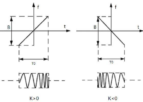
For the pulse compression technique, some kinds of pulses can be used, such as the linear frequency modulated (LFM) signal, the non-linear frequency modulated (NLFM) signal and the phase-coded sig-nal. LFM signal is chosen for pulse compression in SAR. This pulse compression technique maintains both high range resolution of narrow pulses and target detectability of wide pulses [43].

(26)

2.1.2 Geometric Model of SAR

The purpose of this part is to describe a general data acquisition ge-ometric model of SAR and to define some geometry-related terms. Figure 2.3 shows a general model of a SAR regarding radar location and beam footprint illuminated on the Earth’s surface. The SAR im-age formation create an imim-age in slant range (not ground range) and azimuth coordinates.

(27)

In Figure 2.3, The target is a hypothetical point on the Earth’s surface. The SAR systems actually images an area, but this point target is used more easily to develop SAR theories [50]. The radar beam is viewed as a cone and the footprint is the intersection of the cone with ground. The footprint of a single beam is an ellipse, but the whole footprint area will be a stripe on the ground due to the platform moving. The nadir is the point on the Earth’s surface, which is di-rectly below the antenna. Hence, the normal to the Earth’s surface at the nadir passes through antenna. The zero Doppler plane is a plane that is perpendicular to the platform velocity vector direction and the azimuth direction. The intersection of the zero Doppler plane with ground is called the zero Doppler line. The squint angle θsq in the

figure is an angle between the antenna beam pointing direction vec-tor and the zero Doppler plane. If the squint angle is zero, the beam direction vector is perpendicular to the platform velocity vector and the SAR is side-looking. The parameter R is the slant range between antenna and target. During the moving of platform, the distance R will decrease gradually until platform moves to the closest point with target, where R becomes R0, and then it will increase again. Hence,

R0 is calledrange of closet approach when the slant range is minimum

(when the zero Doppler line crosses the target). The line of R0 is

(28)

2.1.3 SAR Signal Properties

In SAR, linear frequency modulated(LFM) signal, which is also called chirp signal, is used for pulse compression. The properties of LFM signal will be introduced firstly. LFM signal is a kind of modulated signals in which the frequency increases or decreases with time. [39]. The relationship of time and frequency of the LFM signal is a linear function. The mathematical equation can be expressed as

s(t) =rect t T0 expj2πfct+ jπKt2 (2.9)

where t is the time variable in seconds, T0 is time duration of the

LFM signal, fc is carrier frequency and K is the linear FM rate in

Hz/s. The instantaneous frequency is the derivative of phase and can be expressed as f = 1 2π dφ(t) dt = 1 2π d(2πfct+πKt2) dt = fc + Kt (2.10)

This means that the frequency is a linear function of time t with the slope K. The waveform of LFM signal is shown in Figure 2.4.

In SAR, both signals in the range and azimuth directions can be considered as LFM signal. Matched filtering approach is used for LFM signal pulse compression. Matched filter is designed to do the correlation process and cancel the quadratic phase term of LFM signal and the equation is given by

h(t) = s∗(−t) = rect t T0 expj2πfct−jπKt2 (2.11)

(29)

Figure 2.4: LFM signal waveform.

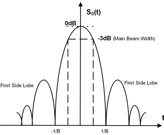
After convolution with matched filter and removing carrier frequency, the output can be given by

s0(t) = s(t)∗h(t) = T0rect t T0 sinc(πBt) (2.12) where the ∗ is the mark of convolution calculation. The waveform of output signal is shown in Figure 2.5. After pulse compression, signal changes to a narrow pulse with unit TBP. Hence, the pulse width of this output signal Tp = _B1 and the compression ratio Kp = T_T0

p = T0B.

It is clear that the final output after pulse compression should be a sinc function. Hence, the output of a point target should be two orthogonal sinc functions in SAR image space.

(30)

Figure 2.5: Output signal after pulse compression.

signal can be given by

spul(τ) = wr(τ)cos 2πfcτ +πKτ2 (2.13) where wr(τ) = rect τ T0

, which is assumed as a rectangular pulse envelope, and τ is the range time (fast time). This LFM signal is transmitted to ground by antenna and reflected by objects on the ground.

Next, we will discuss how the echoes are acquired across a range swath. The radar beam has an elevation beam width in the elevation plane and it is shown in Figure 2.6. The reflected energy at any illu-mination instant is a convolution of transmitted pulse and the ground

(31)

reflectivity gr [9], which can be expressed

sr(τ) = gr(τ)∗spul(τ) (2.14)

where the mark of ∗ means the convolution calculation. Consider a point target at a range distance Ra away from antenna, with the

magnitudeA0, which is back-scattered reflection coefficient σ0. Hence,

the ground reflectivity is gr(τ) = A0δ(τ −2Ra/c), where the 2Ra/c is

the time delay of the signal for reflector. the echo spul(τ) from the

point target is sr(τ) = A0spul(τ −2Ra/c) = A0wr(τ −2Ra/c)cos 2πfc(τ −2Ra/c) +πK(τ −2Ra/c)2 +ψ (2.15)

(32)

In the azimuth direction, we need to consider the Doppler effect to analyze the SAR signal. The geometry side-looking model SAR is shown in Figure 2.7. The slant distance between antenna and point target decreases firstly until the closest slant distance R0, and then

increases again. Assume the coordinate of point target A is (0,Y0,0), va

is the velocity of platform and η is the azimuth time (slow time). Y0 is

the ground range which has a relationship with platform height H and the closest slant distance R0, i.e. Y0 =

p

R2₀ −H2_{. The instantaneous}

slant distance R(η) is given by [12] R(η) =

q

R2₀ +x2 ₌

q

R2₀ + vaη2 (2.16)

In the general case, the closest slant distance R0 is much larger than

the moving distance of platform vaη. Hence, using Taylor series

ex-pansion, the instantaneous slant distance can be approximated as R(η) = q R2₀ +vaη2 ≈ R0 + vaη2 2R0 (2.17) Compared with transmitted pulses, the echoes have time delay and the Doppler frequency shift [12]. Because of the relative motion between platform and point target, the instantaneous phase of the azimuth direction signal is φ(η) = −2π2R(η) λ = −2π v2_a λR0 η2 +Constant (2.18)

where the minus sign is because the echoes lag behind the transmitted pulses. The instantaneous frequency of echoes in the azimuth direction is the derivative of Equation (2.18) and can be expressed as

f(η) = 1 2π dφ(η) dη = − 2v_a2 λR0 η (2.19)

(33)

It is apparent that the instantaneous frequency is a function with time, which can be considered as a LFM signal. Therefore we can also use pulse compression to process azimuth echoes. The relative motion between antenna and point target results in the phase shift with time and linear variation of instantaneous frequency, which is known as Doppler shift. More generally, the instantaneous frequency is

f(η) =fdc +Kaη = −

2v_a2 λR0

η +const (2.20)

where fdc defines the Doppler centroid and Ka is linear FM rate of

azimuth signal. If the working model is side-looking (squint angle is zero), the Doppler centroid is zero. If the working model is not side-looking, the Doppler centroid is a constant.

(34)

After analyzing both the range signal and the azimuth signal, the two-dimensional signal, which is demodulated to baseband, can be expressed as s0(τ, η) =A0wr(τ−2 R(η) c )wa(η−ηc)exp −j4πfcR(η)/c+jπK(τ −2 R(η) c ) 2 (2.21) where the τ is the time in the range direction and the η is the time in the azimuth direction. This equation represents raw data of the point target collected by antenna [12]. Many imaging algorithms, such as the range-Doppler algorithm [5] [26], the chirp-scaling algorithm [44] and the ω−k algorithm [3], have been developed to process raw data and obtain focused images. These algorithms are all based on matched filter to acquire the focused image [50] [12].

According to Equation (2.21), it is obvious that the raw data is two-dimensional. The data of range direction can be processed by pulse compression technique, which is implemented by the matched filter method. The data of the azimuth direction can be seen as the data of an virtual array, which means that the data can be processed by the beamforming method. For a beamforming based processing method, the point target expression can be represented by

s0(η) = A0wa(η −ηc)exp{−j4πfcR(η)/c} (2.22)

where the exponential phase is caused by relative motion between point target and radar. The purpose of processing is to remove the exponential phase of SAR data to acquire clear images. Because the

(35)

raw data in the azimuth direction can be seen as the data collected by an virtual uniform linear array, we can utilize the beamforming method to process data.

2.2

Review of Matched Filter Based Processing

Methods

The Processing of SAR raw data requires a correlation of the col-lected SAR raw data with the reference functions of the azimuth and the range directions. Different reference matched filters are utilized in the azimuth and range directions separately. The 2-D correlator in the time domain can complete the correlation steps, but is computation-ally inefficient [3]. For taking the advantages of fast processing speed in the frequency domain, several processing algorithms have been de-veloped in the decades with different correlation kernels.

The first digital processing algorithm is called range-Doppler al-gorithm, which is developed by J. Bennett and I. Cumming [12] [5]. For more than four decades the range-Doppler algorithm has been the basis of the most accurate and widely used SAR processing al-gorithm [26]. It has three main steps, range compression, range cell migration correction (RCMC) and azimuth compression. Several mod-ifications of this algorithm are proposed to improve its performance. The most important modification is the secondary range compression (SRC), which is used to solve the problem of large squint angle [29].

(36)

The range-Doppler algorithm performs the range compression in the range frequency domain, the RCMC in the azimuth frequency and the range time domain and the azimuth compression in the azimuth frequency domain. This algorithm will be introduced with details and simulation results will be shown in Chapter 3.

In the range-Doppler algorithm, the step of RCMC uses the in-terpolation operation, which requires both computation time and ac-curacy of processed image. The chirp scaling algorithm is proposed by R. Raney to avoid interpolations and perform the RCMC accu-rately [26] [44]. This algorithm modulates the frequency of chirp sig-nal and makes the scaling of chirp sigsig-nal. This is why this algorithm is called chirp scaling algorithm. Phase multiplications using matched filter are used to replace the interpolations that need long computa-tion time in the range-Doppler algorithm. This algorithm requires only complex multiplications and Fourier transform. Compared with the range-Doppler algorithm, chirp-scaling is usually used in large swath and large squint angle scenario. In order to acquire higher accuracy, many modifications based on the chirp-scaling algorithm are proposed, such as the extended chirp scaling (ECS) algorithm [35], the nonlin-ear chirp scaling (NCS) algorithm [15] and the frequency scaling (FS) algorithm [34].

After the chirp-scaling algorithm, a new class of algorithms were then proposed and implemented in order to reduce the approximation

(37)

error further. They are refereed to as the ω − k algorithm, which processes data in the two-dimensional frequency domain [3] [36] [8]. This algorithm is based on Stolt interpolation and can match with the SAR echo signal perfectly. Hence, it has high processing accuracy. In the chirp-scaling algorithm, it uses approximations for SAR data processing, which could be invalid in some scenarios. In order to slove this problem, the ω −k algorithm was formulated in terms of wave equation. The problem of original theω−k algorithm is motion com-pensation is not accurate. In order to solve this problem and make the algorithm more practical, an extend the ω−k algorithm was pro-posed [45] [46].

These algorithms are three main SAR processing algorithms based on matched filter in the frequency domain. They all use some trans-formations and approximations to do the matched filtering in the fre-quency domain. In different applications, they have different modi-fications in order to improve the image quality. In addition to those frequency domain processing algorithms, there is another branch of SAR data processing, which is the time domain processing algorithms. The most typical algorithm is the back-projection algorithm [12]. In theory, this algorithm can match with SAR echo signal perfectly with-out any transformation or approximation. This is the most accurate algorithm based on matched filter. However, extremely large compu-tation time for correlation between the SAR echo signal and reference function matched filter is required. Hence, it is seldom used in

(38)

prac-tice and only used for scenarios with a small observing area.

Based on the theoretical framework of matched filter, many modifi-cations of different algorithms are still being proposed to improve the image quality. However, because of some features of matched filter, the improvement of these algorithms could be limited and these are the limitations of matched filter based algorithms.

2.3

Limitations and Existing Solutions of Matched

Filter Based Processing Methods

2.3.1 Limitations of Matched Filter Based Processing Meth-ods

In general, most of processing algorithms are based on the same the-oretical framework, which is the matched filter. Matched filter is a linear process and easy for implementation. However, it also has sev-eral obvious disadvantages and limitations.

Firstly, The algorithms based on matched filter must obey the Nyquist sampling theorem. In order to avoid distortion of waveform, the sampling frequency must be larger than signal bandwidth. This means the amount of raw data will be much large for a high resolu-tion requirement image. Moreover, because the resoluresolu-tion is related to the signal bandwidth, higher resolution requirement need a higher

(39)

bandwidth. This will result in a higher sampling frequency and it will be a big challenge for the analogue-to-digital converter and the entire hardware system [28].

Secondly, the result of matched filter is a sinc-like function. This means that the image of an ideal point target will be a two-dimensional impluse response with a certain width and the effect of side lobes [12]. Because of this reason, the resolution improvement of matched filter based algorithm could be limited. For two close point targets, they will be distinguishable and ambiguities without any detailed informa-tion. Also, because the main lobes and side lobes of different point targets can affect each other, the image processed by matched filter will have coherent speckle noise and affect the resolution of image.

2.3.2 Existing Solutions for Limitations of Matched Filter

According to the last section, it is clear that what are the problems of the matched filter based processing method. The most significant problem is the high sampling frequency, which results in large amount of sampling points and large amount of stored and processed data, for high resolution requirement imaging. To reduce the amount of sam-pling points (amount of data stored and processed), G. Martino pro-posed a co-prime synthetic aperture radar (CopSAR) [16] [33]. Com-pared with the uniform linear array of conventional SAR, CopSAR uses one kind of sparse array, which is called co-prime array. Co-prime

(40)

array is a combination of two uniform linear arrays with different inter-element spacing. The two values of different inter-inter-element spacing of two arrays are two co-prime number times a constant distanced. This means that they have no common factors except unity. As a result, the elements of two arrays do not overlap. In the proposed algorithm in this paper, a new SAR modality is proposed to transmit two inter-laced sequences of pulses to build the co-prime array. In SAR, pulse repetition frequency (PRF) means the inter-element spacing of arrays. The PRF of conventional SAR corresponds to the aforementioned dis-tance d. This means that the PRFs of two sub-arrays of the co-prime array is smaller than PRF of the conventional SAR. It means that the spacing of inter-element is larger than d. The PRFs of two sub-arrays are smaller than Nyquist frequency. The data received by two sub-arrays are processed by matched filter algorithm separately. This means that the processed images will be severely aliased with many ghost replica targets. Different PRFs will cause different locations of ghost targets in two processed images.

The proposed algorithm in this paper can only be used when the observation area consisting of bright targets on a dark background (such as the scene of ships on the ocean surface), which is similar to the scenario of some point targets. The impulse response of true tar-get will be on the two aliased images at the same locations on the two images. In one of the two aliased images, it shows the replica of tar-get. However, in the other image, it only show the sea background in

(41)

the same location. By comparing the two images, selecting the small-est modulus of two images to remove the replica targets. Conversely, wherever the true target is present, the two images will have similar high moduli. Even a smaller one is selected, the final image still has the correct pixel.

In [33], the authors proposed three modes, which are basic mentation, missing-pulse implementation and dual-frequency imple-mentation. The proposed approach can reduce the amount of data and increase the range swath at the same time without any resolution loss. It is based on adaption of the co-prime array concept to the case of SAR systems. In [17] and [18], G. Martino proposed an improved CopSAR, which is called Orthogonal Co-prime SAR (OrthoCopSAR). This is an improvement of the basic implementation mode of CopSAR, which is based on transmission of (quasi) orthogonal waveforms. This approach can reduce the amount of data and increase the range swath without any ghost target.

These approaches have been tested by using simulated and real data of SAR. It is suitable for ocean and maritime scenario. It is based on co-prime array concept and matched filter. In the other word, these approaches still use matched filter to process data without improving the sampling method. The most significant problem with these ap-proaches is that it is only suitable for scenario of some point targets (ocean ship detection). By using the approach of selecting the lowest

(42)

modulus of two images, the true point target will be removed if it is in the location of replica target of another point target. This means that this approach cannot be used for an image with many high re-flected coefficient targets, such as mapping of the ground. Also, these proposed approaches only use the concept of co-prime array. They do not utilize any array signal processing method such as beamforming or direction of arrival (DoA) estimation in their processing and still use conventional matched filter algorithms to process data. These ap-proaches can be used as a reference to propose new SAR processing method based on array signal processing of co-prime or other kind of sparse arrays.

Another approach to reduce amount of data and mitigate the ef-fect of sidelobes is using the theory of compressed sensing. In recently years, compressed sensing (CS) has been applied in the field of SAR imaging. The reason why SAR cannot reduce the amount of data using matched filter is because we must obey the Nyquist sampling theorem to avoid aliasing. Under the framework of compressed sens-ing, it is possible to reconstruct the sparse or compressible signals with fewer amount of data [10] [4] [19]. Compressed sensing SAR uses priori information of SAR, which is the sparsity of SAR data. In [53], the authors proposed sparse signal representation from complete dictionaries based on the CS theory. In [6], a technique for the com-pression of raw data is proposed based on the use of continuous wavelet transform in order to obtain a sparse representation of the complex

(43)

SAR image. In [22], the authors proposed a method to reduce the amount of stored SAR data based on compressed sensing. In [21], based on the approximated observation, a new SAR fast compressed sensing method is proposed.

Under the framework of compressed sensing, the two main prob-lems are choosing the measurement matrix to represent the SAR signal and choosing different reconstruction algorithms to rebuild signal in different scenarios. The reconstruction in the CS framework is to solve an l0 norm minimization problem. In [20], Donoho points out that

this is a NP-hardness (Non-deterministic Polynomial-time Hardness) problem and difficult to solve. The most common approach is to usel1

norm minimization to replace the original problem. In [9], the authors proved that they could reach the same solution. The first method to solve l1 norm minimization problem is using basis pursuit (BP). This

method can solve the problem based on convex optimization. Another method is called matching pursuit (MP), which is a kind of greedy al-gorithms.

In [7], B. Han proposed a compressed sensing SAR imaging based on co-prime arrays sampling. Co-prime is widely used in the field of DoA estimation and can achieve a higher number of degrees of free-dom. High degrees of freedom means more signal information. This means this co-prime array sampling structure can obtain enough in-formation of the signal by non-uniform low speed sampling. The

(44)

mea-surement matrix is obtained by the transformation of sampling array. In this proposed algorithm, the orthogonal matching pursuit (OMP) greedy algorithm, which is an enhancement of the MP method, is used to reconstruct the signal. Some simulations of several point targets and small area target are shown.

Compressed sensing theory uses the sparsity of SAR signal. Spar-sity means only a small portion of the observing area has targets, such as several point targets or small area target. This means that proposed approaches based on compressed sensing cannot process SAR data of ground mapping, where targets are on the entire observing area. For a scenario that is not sparse, we can use sparse representation to repre-sent SAR data, which means making the SAR data sparse in the other domain. However, the sparse representation for SAR data is difficult because echo signals reflected by different targets have random phase. New approach is still being proposed to solve this problem.

(45)

Chapter 3

SAR Raw Data Processing

Approaches

The raw data received from the radar system must be processed in or-der to acquire focused image. Currently, most of algorithms to process data are based on matched filter. In the time or frequency domain, the matched filter is used to compensate the phase difference of signals received by different sensors (sampling points) of the virtual array. In the following section, one of the most commonly used algorithm, which is called the range-Doppler algorithm, is introduced and simulation re-sults of point target and area target are shown. Then, a introduction of co-prime SAR (CopSAR) is shown with details, which introduces the concept of co-prime array and the CopSAR. Also, some simulation results are presented as follows.

(46)

3.1

The range-Doppler Algorithm

3.1.1 Introduction to the Algorithm

The range-Doppler algorithm processes the raw data calculated from Equation (2.21), which have been first demodulated to baseband, to produce the focused SAR image. This algorithm separately performs pulse compression via the matched filtering in the Fourier transformed range and azimuth domains [26]. For processing time efficiency, the Fourier transforms are processed using fast Fourier transforms (FFTs). Due to the slant range always changes during the motion of platform, this change results in the range cell migration and the coupling be-tween the range and azimuth directions. The range cell migration correction (RCMC) is performed in the range time and the azimuth frequency domain, which is called the range-Doppler domain. This is why this algorithm is called the range-Doppler algorithm. Performing the RCMC in this range-Doppler domain is the defining feature of the algorithm when compared with other processing algorithms. In Figure 3.1, a block diagram of the range-Doppler algorithm is shown. There are three main steps of the range-Doppler algorithm, which are the range compression, the RCMC and the azimuth compression [12].

(47)

(48)

In Section 2.1.3, the matched filtering in the time domain is com-pleted by using the convolution operations. As we known, the convo-lution operations are the same as the multiplication operations in the frequency domain. We only need to transform the raw data and the matched filter reference functions into the frequency domain. Com-pared with the convolution operations in the time domain, the multi-plication operation is much easier in computation so that the process-ing time will decrease dramatically. Hence, all steps of this algorithm are all based on the frequency domain.

Firstly, the two-dimensional signal s0(τ, η) is analyzed as a series

range time signals for each azimuth bin. The equation of this signal is shown in Equation (2.21). The variable τ is the time of the range direction (fast time) and the η is the time of the azimuth direction (slow time). The signals of the range direction are transformed into the frequency domain via FFT, which can be expressed as S0(fτ, η).

The range compression is performed in the range frequency domain. The matched filter in the range frequency domain is defined asG(fτ) =

exp

n

jπfr2

K

o

and is multiplied with signalsS0(fτ, η). The matched filter

is used to remove quadratic phase of signal and compress chirp signal into a sinc function in the range direction. After performing IFFT and transforming back to the range and azimuth time domain, the signals can be represented as

src(τ, η) =IF F Tτ{S0(fτ, η)G(fτ)}

= A0pτ[τ −2R(η)/c]wa(η −ηc)exp{−j4πfcR(η)/c}

(49)

where the compressed pulse envelope pr(τ) is the IFFT of the window

Wr(fτ). For a rectangular window, pr(τ) is a sinc function. For a

tapered window, it will be a sinc-like function with lower side lobes.

Figure 3.2: Signal diagram after range compression [1].

The diagram of signals after range compression is shown in Figure 3.2. The diagram depicts that the signal trajectory of the azimuth direction is curving, which is not in a same range cell. Due to the variation of slant range between the radar and the target, all reflected signals from the target cannot come in a same range cell and follow a hyperbolic trend in the azimuth direction called the range cell mi-gration (RCM). These signals are required to migrate back to a same range cell, which is called range cell migration correction (RCMC).

(50)

In the azimuth time domain, the RCM curves of different targets are different and we cannot correct them at the same time. However, in the azimuth frequency domain, RCM curves of targets with same range distance are same and we can correct them at the same time. This is the reason why the RCMC is performed in the range-Doppler domain [12] [2].

For the low squint cases, the antenna beam points close to zero Doppler direction (side-looking model points to zero Doppler direc-tion). The slant range can be approximated to

R(η) = q R2₀ + V2 aη2 ≈ R0 + v_a2η2 2R0 (3.2) Combining Equation (3.1) and (3.2), the range compressed signal can be given by src(τ, η) ≈ A0pτ[τ− 2R(η) c ]wa(η−ηc)exp{−j 4πfcR0 c }exp{−jπ 2v_a2 λR0 η2} (3.3) According to Equation (2.20), the second exponential phase term in Equation (3.3) can be expressed byexp{−jπKaη2}. It is apparent that

this phase term is quadratic phase and is a function of η2. Then, an azimuth FFT is performed on each range gate to transform the range compressed signal into the range-Doppler domain. The relationship between the azimuth time and the azimuth frequency is

fη = −Kaη (3.4)

(51)

azimuth FFT in the range-Doppler domain can be given by S1(τ, fη) =F F T{src(τ, η)} = A0pr[τ − 2Rrd(fη) c ]Wa(fη −fηc)exp{−j 4πfcR0 c }exp{jπ f_η2 Ka } (3.5) where Wa(fη−fηc) is azimuth beam pattern in the range-Doppler

do-main, the first exponential phase term is the inherent phase informa-tion of target and the second phase term is the azimuth modulainforma-tion. The RCM curve is the term Rrd(fη) and can be approximated by

Rrd(fη) ≈R0 + v_a2 2R0 fη Ka 2 = R0 + λ2R0fη2 8v2 a (3.6) The amount of RCM needed to correct is given by the second term in Equation (3.6). ∆(fη) = λ2R0fη2 8v2 a (3.7) There are two main approaches to implement the RCMC, which are the nearest neighbour interpolation and the sinc function based in-terpolation. The nearest neighbour interpolation performs more effi-ciently but only obtains approximate correction. The efficiency of the sinc function based interpolation depends on the size of interpolator kernel. Longer interpolator kernel can correct more accurately but with a lower efficiency. Usually, a four-point or eight-point interpola-tion is chosen to give a reasonable accuracy [50].

In Figure 3.3, the signal diagram is corrected and becomes parallel with the azimuth direction. There are many sinc function diagrams which are parallel in the direction of azimuth. This does not mean

(52)

Figure 3.3: Signal diagram after the RCMC [1].

that there are many replicas in the direction of azimuth. It means that the signal data can be seen as a sinc function in the range di-rection after range compression, which is the processing result of the first step of the range-Doppler algorithm. All data except the columns that are close to the point target in the azimuth direction can be seen as zero if we ignore the effect of noise. This means that the final im-age will be all black (no reflection) in these areas with data of zero. This is because that the LFM signal in the range direction has been compressed into the sinc function. In the columns that is close to the point target, they will be intensity of the mainlobe and sidelobes of the sinc function in the range direction after the range compression.

(53)

Assuming the RCMC is applied accurately, the signal after the RCMC can be represented by S2(τ, fη) =A0pr(τ − 2R0 c )Wa(fη −fηc)exp{−j 4πf0R0 c }exp{jπ f_η2 Ka } (3.8) It is apparent that the range envelope sinc function pr becomes

inde-pendent of the azimuth frequency, which means the RCM has been corrected.

After the RCMC, a matched filter is used to implement the azimuth compression in the azimuth direction to complete pulse compression in the azimuth direction. It is convenient to implement azimuth com-pression in the Range-Doppler domain. Similar with the matched filter in the range direction, the azimuth matched filter is the complex conjugate of the second exponential phase term in Equation (3.5) to remove quadratic phase in the azimuth direction and can be given by

Haz(fη) =exp ( −jπ f 2 η Ka ) (3.9) where Ka is the azimuth linear FM rate shown in Equation (3.4). An IFFT is then completed after the azimuth compression. The final signal is given by sac(τ, η) = IF F Tη{S2(τ, fη)Haz(fη)} = A0pr(τ − 2R0 c )pa(η)exp −j4πfcR0 c exp{j2πfηcη} (3.10) where pa is azimuth impulse response, which is a sinc-like function

(54)

focused and positioned at τ = 2R0/c and η = 0. These two envelopes

are orthogonal, which is shown in Figure 3.4, so that we can acquire a focused point in the image space. There are two exponential phase terms in Equation (3.10). The first term is target phase which de-pends on range position and the second term is a linear phase which depends on the Doppler centroid [13] [12].

Figure 3.4: Signal diagram after the azimuth compression [1].

Compared with Figure 3.3, Figure 3.4 shows the final SAR image of a point target by using the processing algorithm of the range-Doppler algorithm. In Figure 3.3, the data is a sinc function in the range direc-tion. However, the data in the azimuth direction is still LFM signal with a rate of Ka. It is difficult to show this in a diagram but we can

(55)

know it from the Equation (3.8). In Figure 3.4, the LFM signal in the azimuth direction is compressed to the sinc function as well. Hence, the final SAR image shows two orthogonal sinc functions in the posi-tion of point target. This means that all data except the column and row of the point target should be zero in theory. The final image of a point target in the SAR image space should be a cross which has a centre in the position of the point target.

3.1.2 Simulation Results

Firstly, a simulation sample of the range-Doppler algorithm is given to acquire a point in the image space. In this simulation, the ob-servation area is from Xmin = −400m to Xmax = 400m in the

az-imuth direction. The central line of observation area in the range direction is Yc = 10000m and the area in the range direction is from

Yc −Yw = 9400m to Yc +Yw = 10600m. The moving velocity of

plat-form is v = 100m/s and the height is H = 5000m. The resolution of range and azimuth direction are both set to ρr = ρa = 2m. The

sampling points in the azimuth and range direction are Na = 2048

and Nr = 1024. The coordinate of target point is (0, Yc), which is the

center location of the observation area.

Figure 3.5 shows the intensity of the point target. In Figure 3.5, high intensity is represented by yellow and low intensity is represented by blue. From this figure, we can find that the location of point

(56)

tar-get has a high amplitude intensity. However, there are also many sidelobes in the surrounding locations in the both azimuth and range directions. These sidelobes could make the image distorted. If another point target with low intensity is on the adjacent location of this high intensity point target, the point with low intensity will be covered by the sidelobe of the high value point because the intensity of sidelobe could be higher than the low value point target. This situation will make the processed image distorted and the image could be different from the real image of ground.

Figure 3.5: Intensity of the point target.

(57)

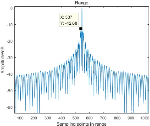
in the range and azimuth directions, respectively. In these two figures, we can analyze the performance of this range-Doppler algorithm. The 3dB width of main lobe is the real resolution of this image. From these two figures, the azimuth resolution is 3m and the range resolution is 3.5m. Compared with theoretical resolution 2m, the real resolution of processed image is worse than theoretical calculation. This means that the quality of processed image could be worse than expected. SAR has a ratio to analyze the performance of sidelobe effect, which is called the peak sidelobe ratio (PSLR). It is a ratio of maximum in-tensity of mainlobe and maximum inin-tensity of strongest sidelobe. In these two figures, the PSLR values of the range and azimuth direction are provided, which are -12.68dB in the range direction and -12.90dB in the azimuth direction. These two values of PSLR are acceptable and this means that we can obtain a clear SAR image. The simulation of an area target is introduced in the following part.

(58)

Figure 3.6: Impulse response (point target result) in the range direction.

(59)

Secondly, a simulation of area target is shown as follows. A pic-ture or photo is created by many discrete pixels (points with different grayness degrees). Similarly, the area target is equivalent to many point targets with small distance which is smaller than resolution. In this simulation, the observation area in the azimuth direction is still Xmin = −400m and Xmax = 400m. The observation in range

direc-tion is from Yc −Yw = 9400m to Yc+Yw = 10600m, which are all the

same as the point target simulation. Other parameters are also the same as the simulation of point target. However, the sampling points of the azimuth and range direction are changed to Na = 512 and

Nr = 1024. A Google satellite map photo is set in the center area of

observing area, which has a size of 601x701, which is shown in Figure 3.8. This means that there are totally 421301 discrete point targets with adjacent distance of half of theoretical resolution, which is 1m. These point targets build a rectangular area target on the center area of observing area. Different point target has different back-scattered reflection coefficient, which is correspond to the grayness degree of pixel in the map photo. Other locations in the observation area all have no target with no reflections. This means that these area will be all black in the processed SAR image.

Figure 3.9 shows the simulation result of the area target. From this image, many details of input image can be distinguished. However, it is obvious that the quality of this reconstructed image is worse than the input image in Figure 3.8. This is because the real resolution of

(60)

this image is worse than the theoretical resolution. Also, the quality of image is influenced by the effect of side lobes. This area target sim-ulation result is the same as the analysis of the point target (impulse response) in the above part.

(61)

Figure 3.8: Input image of the area target [49].

(62)

3.2

Co-prime SAR Concept and Simulations

3.2.1 Introduction to Co-prime Array and CopSAR

In this research, the most significant aim is to reduce the amount of raw data. We can use the concept of sparse array in the array sig-nal processing. The sparse array is a concept which is different from the ULA. The ULA has fixed distance between two adjacent sensors. However, the sparse array has different distance between different two sensors. This means that sparse array uses fewer sensors than the ULA in a same length of array. We can exploit the second order sta-tistical information to receive a smaller performance compared with the ULA. However, the amount of data decreases because the amount of sensors decreases. The co-prime array uses two co-prime integers in two sub-arrays. In Figure 3.10, for two sub-arrays with two co-prime integers, they share the same sensor in the first position and they will share the same sensor again until the M N − th position because M and N are co-prime. This means that we can generate an virtual array with consecutive integers from -M(N-1) to M(N-1), which is a larger virtual ULA with better performance. This is why we are going to utilize the co-prime array in SAR as well.

The concept of co-prime array will be introduced in deails in the following parts. Co-prime array is one kind of sparse arrays. The co-prime array consists of two uniform linear sub-arrays with distance M d and N d respectively, which is shown in Figure 3.10. There are

(63)

M sensors in the first sub-array and N sensors in the second sub-array where M and N are co-prime integers, for example, 4 and 5. In the location of 0, two sub-arrays share same sensor. Except this sensor, two sub-arrays have separate ULA pattern with different spac-ing. d is the unit of inter-element spacing. For uniform linear array (ULA), d is typically set to λ/2 or smaller than λ/2 to avoid spatial aliasing [51] [54]. However, it is obvious that distance between two adjacent sensors of the co-prime array is larger than d.

Based on the sparse array signal processing, we can build an vir-tual ULA. Based on the concept of difference co-array, an virvir-tual ULA with 2M(N−1) + 1 virtual sensors can be generated. The virtual sen-sors are corresponding to the consecutive integers from−M(N−1) to M(N−1). This operation leads to a significant increase in the degrees of freedom, which means co-prime array can receive same performance with fewer sensors (fewer sampling points and fewer amount of data in SAR) [51].

(64)

Figure 3.10: A general co-prime array structure.

For the co-prime SAR, it uses the concept of co-prime to reduce the sampling points, which reduces the amount of the raw data stored and increase the range swath [16]. Because this approach is still based on matched filter, the sampling must obey the Nyquist sampling the-orem. This means that the sampling frequency must higher than the bandwidth of signal. In the azimuth direction, the bandwidth is the SAR signal Doppler bandwidth, i.e., its Nyquist rate. Usually, in or-der to avoid the aliasing, the selected PRF of conventional SAR must be larger than the Doppler bandwidth, which can be represented as

P RF0 ≥

2v

L (3.11)

where v is the velocity of SAR platform and L is the real length of antenna. However, the PRF of co-prime array must be smaller than theP RF0 because the distance between two adjacent sensor increases.

(65)

For example, if the two co-prime integers are 4 and 5, the structure of CopSAR are shown in Figure 3.11. The blue point is the first sub-array with M = 4, which means its P RF1 = P RF0/M. The other red

points are the second sub-array withN = 5 and theP RF2 = P RF0/N.

Because two integers are co-prime, the array will repeat the pattern each M N = 20 sensors. To calculate the reduction of raw data, a ratio R is defined between the number of pulses transmitted by the CopSAR and the number of pulses transmitted by the conventional SAR.The ratio R can be expressed as

R = 1 P RF0 (P RF0 M + P RF0 N − P RF0 M N ) = M +N −1 M N (3.12)

Figure 3.11: Structure of the CopSAR concept.

The PRF of CopSAR is lower than the Nyquist rate, the replica ghost targets will be displayed on the image space.The shift of replicas in the azimuth direction and the range direction can be calculated by the following equations:

∆xi = i P RF0λr0 2v (3.13) ∆ri = ∆x2_i 2r0 (3.14) where λ is the wavelength, r0 is the closest slant range between the

radar and the target. Two sub-arrays can be used to produce two separate SAR images. This means that they should use different PRF

(66)

to calculate replicas in different SAR images. For the first sub-array, each target gives rises to replicas displayed as

∆xi1 = i1 P RF0λr0 M2v (3.15) ∆ri1 = ∆x2_i₁ 2r0 (3.16) For the second sub-array, each target gives rise to replicas displayed as ∆xi2 = i2 P RF0λr0 N2v (3.17) ∆ri2 = ∆x2_i₂ 2r0 (3.18) The resolution of these two processed images are the same as the con-ventional SAR because the synthetic array length of CopSAR is the same as the conventional SAR. But because of the low sampling fre-quency, these two images are severely aliased. According to aforemen-tioned equations, replicas on the two images will at different locations, unless it is the real target. To combine these two aliased images, we can choose the smaller modulus at each pixel, the replica ghost targets will be removed. The choosing step can be represented as

s(x, r) =      s1(x, r), if|s1(x, r)| < |s2(x, r)| s2(x, r), otherwise (3.19)

Because this CopSAR is used in the scenario of ocean ships detection, a replica in the location of one aliased image, the same location of an-other aliased image must be dark and without any replica. The final images(x, r) with no replica can be obtained. In one of the two aliased

(67)

images, there is a replica ghost of the target. In the other aliased im-age, it should be darkness with low modulus (sea background). By choosing the smallest modulus of the two aliased images, the replica ghost targets can all be removed. Some simulation results of CopSAR are shown in the following subsection.

3.2.2 Simulation Results

Firstly, a simulation of single point target is provided. The parameters are the same as the area target simulation in the section 3.1.2. The two co-prime integers are the same as the aforementioned example, which are 4 and 5. The conventional SAR P RF0 = 94.858Hz. The PRF of

two sub-arrays are P RF1 = 23.7145Hz and P RF2 = 18.9716Hz,

re-spectively. These two PRF are lower than Nyquist rate and will result in severely aliased. The point target is set on the center of observing area, which is (0,Yc). The aliased image s1(x, r) is created by the first

sub-array and the s2(x, r) is created by the second sub-array. The

final images12(x, r) is created by combining s1(x, r) and s2(x, r) using

(68)

960 980 1000 1020 1040 1060 1080 1100

Sampling points in range

460 470 480 490 500 510 520 530 540 550 560

Sampling points in azimuth

Figure 3.12: Intensity of point target processed by the CopSAR.

In Figure 3.12, a point target processed by CopSAR is shown. Com-pared with simulation result of conventional SAR, it has similar per-formance of resolution and side lobes. However, the amount of data decreases significantly compared with conventional SAR. In the con-ventional SAR, the sampling points of this simulation is 1024. For this CopSAR, the number of sampling points in the first sub-array is 256 and the number is 205 in the second sub-array. This means that there are 461 sampling points totally. This is a significant reduction compared with the conventional SAR. Because the PRF reduces, the range swath also increases without any loss of geometric resolution.

(69)

Figures 3.13 to 3.16 show the impulse response (point target re-sult) of the first sub-array aliased image, the second sub-array aliased image, the combined image and the conventional SAR image, respec-tively. According to Figures 3.13 and Figure 3.14, it is obvious that the location of replica ghost targets are different for different sub-arrays. Hence, by choosing the smallest modulus of each pixel, we can achieve the final image in Figure 3.15. Compared with the image of conven-tional SAR, it has small sidelobes around the point target but it can be ignored because it is relatively much lower than the mainlobe of the point target. This means that this approach CopSAR can achieve similar performance of image quality but with a significant reduction of data amount and increase of range swath.

(70)

-400 -300 -200 -100 0 100 200 300 400 Azimuth observation area/ meter

0 0.1 0.2 0.3 0.4 0.5 0.6 0.7 0.8 0.9 1

Impulse response function

s1 Azimuth

Figure 3.13: Impulse response (point target result) ofs1(x, r) in the azimuth

direc-tion.

0 0.1 0.2 0.3 0.4 0.5 0.6 0.7 0.8 0.9 1

s2 Azimuth

(71)

0 0.1 0.2 0.3 0.4 0.5 0.6 0.7 0.8 0.9 1

s12 Azimuth

direc-tion.

0 0.1 0.2 0.3 0.4 0.5 0.6 0.7 0.8 0.9 1

Standard Azimuth

Figure 3.16: Impulse response (point target result) of the conventional SAR in the azimuth direction.

(72)

The second simulation is to simulate a ship target with length of 100m, which is a long target with many point targets. The parame-ters of simulation are all the same as the point target simulation. In Figures 3.17 and 3.18, the simulation results of CopSAR and conven-tional SAR are compared.

Compared with the point target simulation result of the conven-tional SAR, the result of CopSAR has some small replicas in the image. This is because the replica ghost targets also have sidelobes. Some replica sidelobes of these two aliased images coincide in the same locations and cannot be removed perfectly. This situation results in that the replica ghost targets cannot be remove completely using the approach of Equation (3.19). However, the modulus is much lower compared with the real target and can be ignored and seen as noise in the final image. Furthermore, we can compare the data amount of this two approaches. The conventional has 1024 sampling points. The CopSAR has 256 sampling points in the first sub-array and 205 sampling points in the second sub-array. There are only 461 sampling points totally in the CopSAR, which is only 45% of the data amount in the conventional SAR. It is obvious that the CopSAR has a bet-ter advantage of data amount in some scenarios (ship detection and surveillance in the ocean).

(73)