Abstract—Extracting information from a training data set for predictive inference is a fundamental task in data mining and machine learning. With the exponential growth in the amount of data being generated in the past few years, there is an urgent need to develop or adapt existing learning algorithms to efficiently learn from large data sets. This paper describes three scaling techniques enabling machine learning algorithms to learn from large distributed data sets. First, a general single-pass formula for computing the covariance matrix of large data sets using the MapReduce framework is derived. Second, two new efficient and accurate sampling schemes for scaling down large data sets for local processing are presented. The first sampling scheme uses the single-pass covariance formula to select the most informative data points based on uncertainties in the linear discriminant score. The second technique on the other hand selects informative points based on uncertainties in the logistic regression model. A series of numerical experiments demonstrates numerically stable results from the application of the formula and a fast, efficient, accurate and cost effective sampling scheme.
Index Terms—Linear discriminant analysis, logistic regression, classification, sampling, mapreduce, single-pass.
I. INTRODUCTION
The basic machine learning task is that of extracting relevant information from a training set for predictive inference. Given today's ever and steadily growing data set sizes, the machine learning process must be able to effectively and efficiently handle large amounts of data. However, most existing machine learning algorithms were designed at a time where data set sizes were far smaller than current sizes. This has led to a significant amount of research in scaling methods, that is, designing algorithms to efficiently learn from large data sets. Two general approaches can be identified in this endeavor: scaling up and scaling down.
The first approach attempts to scale up machine learning algorithms, that is, develop new algorithms or modify existing algorithms so that they can better handle large data sets. There has been a rapid rise in research methods for scaling up machine learning algorithms. This research has been aided in part by the fact that some machine learning algorithms can be readily deployed in parallel. For example [1] showed that ten commonly used machine learning algorithms (logistic regression, näive Bayes, k-means clustering, support vector machine etc) can be easily written as MapReduce programs on multi-core machines. The other Manuscript received September 19, 2013; revised December 10, 2013. Che Ngufor is with Computational Sciences and Informatics at George Mason University, Fairfax, VA (e-mail:[email protected]).
Janusz Wojtusiak is with the George Mason University Department of Health Administration and Policy (e-mail:[email protected]).
part can be attributed to the rapid evolution of hardware and programming architectures [2]. These new technologies are highly optimized for distributed computing in the sense that they are parallel efficient, reliable, fault tolerant and scalable. The Hadoop-MapReduce framework for example has been successfully applied to a broad range of real world machine learning applications [3], [4].
Despite the appealing properties of scaling up machine learning algorithms, there are some obvious problems with this approach. First, scaling up an algorithm so that it can handle "large" data today does not necessarily mean it will handle "large" data tomorrow. Second, adapting current algorithms to cope with large data can be very challenging and the scaled-up algorithm may end up being too complex and computationally very expensive to deploy. Finally, not all machine learning algorithms can be modified for parallel implementation. Coupled with the fact that there is no single algorithm that is uniformly the best in all applications, it is sometimes necessary to deploy many algorithms so that they can collaborate to improve accuracy.
The second approach to the scaling problem attempts to scale down large data sets to reasonable sizes that allow practical use of existing algorithms. The traditional approach is to take a random sample of the large data for learning. This näive approach can run the risk of learning from non-informative instances. For example, in imbalance classification problems where one class is underrepresented, it is possible for random sampling to select only a few members of the minority class and a large number of the majority class, presenting yet another imbalance learning problem.
Though not exhaustively explored, research in methods for scaling up algorithms have been on the rise in the past few years. Not much work has been done in finding efficient ways to scale down very large distributed data sets for learning.
This work presents three key contributions to the research in learning from large distributed data sets. In a first step, a new single-pass formula for computing the covariance matrix of large data sets on the MapReduce framework is derived. The formula can be seen as an efficient generalization of the pairwise and incremental update formula presented in [5]. The single-pass covariance matrix estimation is then used in a second step to derive two new sampling schemes for scaling down large distributed data set for efficient processing locally in memory. Precisely, uncertainties in the linear discriminant score and the logistic regression model are used to infer the informativeness of data points with respect to the decision boundary. The informative instances are selected through uncertainties of interval estimates of these statistics.
Because real data is not always normal, linear discriminant analysis (LDA) may perform poorly when the normality assumption is violated. Thus the Hausman specification test
Learning from Large Distributed Data: A Scaling Down
Sampling Scheme for Efficient Data Processing
Che Ngufor and Janusz Wojtusiak
[6] can be applied to test for normality and decide which sampling scheme to use. The Hausman test requires consistent estimators of the asymptotic covariance matrix of parameters of the models to be tested. The fisher information matrix is easily computed from the output of the logistic regression (LR) and provides a consistent estimator of the asymptotic covariance matrix of the parameters. On the other hand, consistent estimators of the asymptotic covariance matrix of parameters of LDA are not readily available. To solve this problem, this paper also derives a consistent asymptotic covariance matrix of the parameters of LDA that is simple and easy to compute for large data sets using the single-pass covarinace formula.
Empirical results show that using these techniques, large classification data sets can be efficiently scaled down to manageable sizes permitting local processing in memory, while sacrificing little if any accuracy. There are also many potential benefits of the sampling approach: The selected samples can be used to gain more knowledge about the characteristics of the decision boundary, for visualization and to train other algorithms that cannot be easily trained on MapReduce. A specific example to illustrate the usefulness of this approach is presented where the support vector machine (SVM) is trained using scaled down data and large scale predictions is carried out on MapReduce.
For simplicity, this paper considers only binary classification problems and organized as follows: Related work is presented in Section II. Section III presents a general single-pass formula for computing the covariance matrix of large data sets. Section IV briefly reviews LDA and LR and presents confidence interval estimates of the models. Derivation of the asymptotic covariance matrix of parameters of LDA is also presented in this Section. Implementation of the single-pass covariance matrix computation and the proposed sampling schemes on MapReduce is presented in Section V. Numerical experiments are reported in Section VI while Section VII concludes the paper.
Because of space limitations, the proofs of the propositions presented in the paper will be omitted. The interested reader is referred to http://www.mli.gmu.edu/publications for proofs and other detailed information.
II. RELATED WORK
Single-pass pairwise updating algorithms especially for the variance have been in existence for some time and proven to be numerically stable [5]. In these techniques, the data set is always split into two subsets and the variance/covariance of each subset computed and combined. This leads to a tree like structure where each node is the result of the combination of two statistics each of which resulted from the combination of two other statistics and so on. The draw back of these methods lies in the pairwise incremental updating step. At each round of the computation, the data is split into two and the formula is applied recursively. Some special data structures and bookkeeping may be required to handle the tree-like structure of the algorithm. More over, it is not readily amenable to the MapReduce framework as some communications between processes may be required. The single-pass formula presented in this paper avoids the tree like combination structure and computes the covariance matrix in one step.
Much work has been done on scaling up existing machine learning algorithms so that they can handle large data sets and reduce execution time. While this approach is attractive, they are many situations where it is not possible to scale up a machine learning algorithm or the scale up may produce a complex or computationally more expensive algorithm. In such situations, scaling down by sampling is an attractive alternative. Various approaches have been followed to reduce training set sizes such as dimension reduction, random sampling, active learning [7] etc. The simplest of these sampling techniques is random sampling in which there is no control of the nature and type of instances that are added to the training set. It is possible to reduce training size with random sampling and end up with a training set with no precise decision boundary. It is therefore important to guide random sampling so that the reduced training set always has classes separated by a precise decision boundary.
Active learning on the other hand is a controlled sampling technique that has been shown in several applications to be reasonably successful in dealing with the problem of acquiring training data. Its main purpose is to minimize the number of data points requested for labeling there by reducing the cost of learning. In active learning using SVM for example [7], training size reduction is archived by training a classifier using only the support vectors or data points close to the SVM hyperplane. A major drawback of using SVM for sample size reduction is that training SVM is at least quadratic in the training set size. Thus, the computational cost for large data sets can be very significant. In addition, SVM is also known to be very difficult to parallelize especially on MapReduce where there is little or no communication between processes.
The sampling schemes for sample sized reduction presented in this work are designed to avoid or minimize these problems.
III. SINGLE-PASS PARALLEL STATISTICS
Accurate computation of statistics such as the mean, variance/covariance matrix and the correlation coefficient/matrix are critical for the deployment of many machine learning applications. For example, the performance of discriminant analysis, principal component analysis, outlier detection, etc . depends on the accurate estimation of these statistics. However, the computation of these statistics especially the variance or covariance matrix can be very expensive for large data sets and potentially unstable when their magnitude is very small. The standard approach consist of calculating the sum of squares deviation from the mean. This involves passing through the data twice, first to compute the mean and second the deviations from the mean. This naive two-pass algorithm is known to be numerically stable, but may become too costly.
Single-Pass Covariance Matrix Formula
Given a large distributed data set that can be partitioned into k2 finte blocks k1
i i
with ,
i j i j. Each iis typically a set ofni multivariate random samples i {X1,,Xni} where each Xi is a p1
random vector: 1 ( , , ) p T i i i
X X X . The scatter matrix for
each block is given by ( )( )
i T i
X XXi XXi S , where 1/ i X i X X n
is the sample mean of each block. Unbiased estimate of the covariance matrix of each block is given by Σˆ 1/ ( ni1)Si. The main goal is to compute thecovariance matrix of the complete data .
Proposition 1. The scatter matrix of the distributed data partitioned into k2 disjoint data-blocks { }k1
i i is given by 1 1 1 2 1 2 1 1 ( )( ) k T i i n n X X X X n
S S (1) where 1 , 1/ i i i i k i X n n X n X
and
( )denotes the summation over
2k combinations of distinct pairs ( , 1 2) from (1,, )k .IV. SCALING DOWN SAMPLING SCHEMES
In most classification problems, the classifier usually has great uncertainty in deciding the class memberships of instances on or very close to the decision boundary. These are interesting data points warranting further investigation. If the classifier can be taught how to accurately classify these points, then classifying the non-boundary points will be a trivial process. It is well known in the active learning community that training a classifier only on the most uncertain examples can drastically reduce data labeling cost, computational time and training set size without sacrificing predictive accuracy of the classifier [7]. Borrowing this idea, this section presents two complementary sampling schemes based on the linear discriminant score and the logistic regression model to scaled down large distributed data set for local learning.
A. A Linear Discriminant Score Sampling Scheme LDA aim at discriminating between two multivariate normal populations with a common covariance matrix
1 p( , )1
H μ Σ and H1 p(μ Σ2, ) say, on the basis of independent random samples of sizes n1 and n2. Fisher's linear discriminant rule assigns a new test example
x
into population H1 if the discriminant score ( )x satisfies( ) 0 T 0 x x λ (2) where 1 0 2 1 2 1 2 1 1 log( / ) ( ) ( ), 2 T μ μ Σ μ μ 1 2 1 ( )
λ Σ μ μ and i is the probability that
x
belongs to population Hi.The decision boundary is defined by points satisfying
( )x 0
. If the true value of ( )x is known, then these points can be easily determined. However ( )x is not known
and is usually estimated using unbiased sample versions such as the minimum variance unbiased estimator [8] given as
2 2 2 1 2 1 1 1 ˆ( ) ˆ ( ) ˆ ( ) log( / ) 2 2 x x x n n (3) where 2 1 1 2 ˆ ( 3)( )T ( ) / i n n p x Xi p x Xi p ni S
with Xi the sample mean and Spthe pooled covariance matrix. If the probability distribution of ˆ( )x is known, then one can easily find the likelihood that the true value of the score is within some specified range for each test point
x
. For example if ˆ( )x is assumed to be normally distributed, then a 95% confidence interval centered at 0 will correspond to data points close to the decision boundary.The LDA sampling scheme presented in this work is based on an approximate distribution derived in [8] under the assumption of equal priors i.e 12. The case of unequal priors can be adjusted accordingly.
Letting 2 1
( ) ( )T ( )
i x x i x i
μ Σ μ be the squared
Mahalanobis distance between
x
and the population centeri μ and 2 1 2 2 1 1 ( ) ( ) ( ) 2 2 x x x , it is shown in [8] that ˆ( )x
is asymptotically normally distributed with mean ( )x and variance var(ˆ( )x) given (in a simplified form) as:
2 2 4 2 1 2 1 2 2 2 ˆ ( ( )) ( ( ) / (2 )) ( )( / ( )) ( ) / 4 2 ( ) / ( 1) / a var x x cM n b b x cN n a bc p N M n c M n d μ μ (4) where N n1 n2, M n2n1 , nn n1 2 , a N p 1 , 2 b a , c N 2 and d(a1)(b2).With the approximate distribution of ˆ( )x , uncertainties in classifying each data point x can be estimated by computing confidence intervals about the mean value ˆ( )x . In particular, the (1)100% confidence interval about the decision boundary ( )x 0 is given by
2 2 1 1 ˆ( ) ˆ ( ( )) x var x Z Z (5)
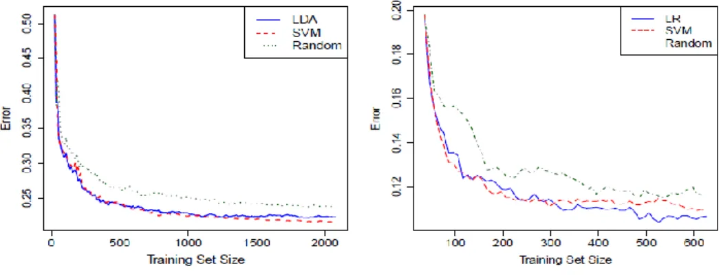
Fig. 1. Performance of sampling schemes.
Data points within this interval represent points for which the classifier has high uncertainty about class memberships and are the most informative for learning. A large confidence interval will select more points while a tight interval will return fewer points. Equation 5 therefore presents an efficient principled query strategy for uncertainty base active learning [7] that can be used for sample size reduction.
In the standard pooled based active learning parlance, a small labeled training set l and a large "unlabeled" pool
u are assumed to be available. The task of the active learner
is to use the information in l in a smart way to select the best query point *
u
x and ask the user or an oracle for its label and then add to l. This process continues until the desired training set size or accuracy of the learner has been archived. For the sampling schemes proposed in this work however, both l and u are labeled training sets, and the idea is to select the most informative data points and their labels from u. The proposed learning algorithm for sample size reduction is presented in Algorithm 1.
The stopping criterion of the algorithm can be set equal to the required sample size of the reduced training set. Note that at each round of the algorithm, the selected points can be used to train a different classifier such as LR or SVM. Fig. 1(a) shows a comparison of the classification performance of LR trained at each step of the sampling scheme using: data points selected by LDA sampling scheme, the support vectors from a SVM training, and random sampling (Random).
The forest covertype data from the UCI Machine learning repository [9] was used for training. The classification problem represented by this data is to discriminate between 7 forest cover types using 54 cartographic variables. The data was converted to binary by combining the two majority forest cover types (Spruce-Fir with n = 211840, and Lodgepole Pine with n = 283301) to one class and the rest (n = 85871) to the second class. The data was split into 75% training and 25% testing. The sampling schemes were stopped once 0.7% of the training set has been queried for learning. The results showed that for the LDA sampling scheme, to archive a reduction in error of about 22% (approximately where the algorithm stabilizes) only about 0.23% carefully selected training data points were needed whereas random sampling method uses all 0.7% of the training data and still achieved only 0.24 % reduction in error. The performance of LDA and SVM sampling schemes are very similar, however LDA took by far a smaller time to converge compared to SVM.
Precisely in this example, the time ratio of SVM to LDA was about 140 averaged over ten fold cross-validation.
To the best of the knowledge of the authors of this paper, this is the first "active" learning technique for sample size reduction based on uncertainties in the linear discriminant score.
B. A Logistic Regression Sampling Scheme
LR is another popular discriminative classification method that makes no assumption about the distribution of the independent variables. It has found wide used in machine learning, data mining, and statistics.
Let {( , )}n1 i i i
x y
be a set of training examples where the random variables Yiyi (0,1) are binary and
p i i
X x are p -dimensional feature vectors. The fundamental assumption of the LR model is that the log-odds or "logit" transformation of the posterior probability
( ; )x Pr(y 1| ; )x β β is linear i.e log 0 1 T x β (6) where 0and β( ,i ,p) are the unknown parameters of
the model.
Typically, the method of maximum likelihood is used to estimate the unknown parameters. By setting x: (1, ) x and
0
: ( , )
β β the regularized log-likelihood function is given by
2 1 ) log 1 exp( | ( ) || | n T T T i i l x
β β X Y β βwhere X is the design matrix, Y the response vector and reflects the strength of regularization. Iterative methods such as gradient based methods or the Newton-Raphson method are commonly used to compute the maximum likelihood estimates (MLE) βˆ of β. For example, the one step training of L2 -regularized stochastic gradient descent (SGD) is given by
new old ( old) old
i i i
y x
β β β β (7)
consist of choosing an example ( ,x yi i) at random from the
training set and updating the parameter β.
An important feature of the LR parameters is that the parameter estimates are consistent. It can be shown that the MLE of LR are asymptotically normally distributed i.e
ˆ
1
, ( )
n β β O I β
where ( ) T
I β X WXis the Fisher information matrix with
{ (1i i)}, 1, ,
diag i n
W (see for example [10]
Section 6.5). Based on the distribution of βˆ, the asymptotic distribution of the MLE of the logistic function ˆ can be derived by application of the delta method. Specifically, for any real valued function g with the property that g( ) /β β
one has
ˆ
1
( ) ( ) , ( ) ( )T ( )
n g β g β Ogβ I β g β
where is the gradient operator. By taking g( )β ( ; )β x , it can be seen that ˆ ( ; )βˆ x is asymptotically normally distributed with mean ( ; )β x and variance
ˆ
1( ; ) ( ; ) ( )T ( ; )
x x
Var β β I β β x .
The decision boundary of LR model is defined by
0 0
T
x
β i.e where ( ; )β x 0.5. This shows that points on the boundary have equal chances of being assigned to either population. Therefore, uncertainties in ( ; )βˆ x for the boundary points can be statistically captured by a
)
1 0%
( 10 confidence interval about 0.5.
Confidence intervals for parameter estimates of LR can be calculated from critical values of the student t-distribution. By following a similar calculation presented in [11] Section 8.6.3 for computing the confidence interval of a linear function T
a β of parameters of a linear regression model, one obtains for ( ; x)βˆ the statistics:
ˆ ( ; ) ( ; ) ~ ( 1) ˆ ( ; ) t Va x x t r n p x β β βwhich has a student t-distribution with n p 1 degrees of freedom. Uncertainties about the true decision boundary
( ; )x 0.5
β can now be inferred through confidence intervals. In particular, the (1)100%confidence interval about the decision boundary is given by
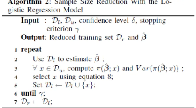
, 1 , 1 2 2 ˆ ( ; ) 0.5 ˆ ( ; ) n p n p x Var t x t β β . (8)A similar algorithm for sample size reduction using the logistic regression model is presented in Algorithm 2.
Fig. 1 (b) shows the error curve for the logistic regression trained at each step of the sampling scheme using: data points selected by the LR sampling scheme, the support vectors from a SVM training, and random sampling. The Waveform data set from the UCI machine learning repository was used for this example. There are a total of 5000 records in this data set with 40 attributes, 75% was used for training and 25% for testing. All the sampling schemes were stopped once 16% of the training set has been queried for learning. Clearly, the LR sampling scheme outperforms both the SVM and Random schemes.
The authors of this paper are unaware of any previous use of uncertainties in the LR model as described in Algorithm 2 for sample size reduction or for active learning. A closely related but different approach is the variance reduction active learning for LR presented in [12]. The idea of this approach is to select data points that minimizes the mean square error of the LR model. To do this, the mean square error is decomposed into its bias and variance components. However, in the active learning step, only the variance is minimized and the bias term neglected. Frequently however, the bias term constitutes a large portion of the model's error, so this variance only active learning approach may not select all informative data points.
C. The Hausman Specification Test
Under the normal assumption, LDA and LR estimators are known to be consistent but LDA is asymptotically more efficient [13]. Thus the Hausman specification test can be applied to test for these distributional assumptions by comparing the two estimators. This section briefly presents the derivation of the asymptotic covariance matrix of the LDA parameters required for the Hausman specification test. This is useful in deciding which of the sampling schemes presented in this paper is best to use.
The LDA and LR models are very similar in form but significantly different in model assumptions. LR makes no assumptions about the distribution of the independent variables while LDA explicitly assumes a normal distribution. Specifically, LR is more applicable to a wider class of distributions of the input than the normal LDA. However, as illustrated in [13], when the normality assumption holds, LDA is more efficient than LR. Under non-normal conditions, LDA is generally inconsistent whereas LR maintains its consistency. Since LDA may perform poorly on non-normal data, an important criterion for choosing between LR and LDA is to check whether the assumption of normality is satisfied.
The Hausman's specification test is an asymptotic chi-square test based on the quadratic form obtained from the
difference between a consistent estimator under the alternative hypothesis and an efficient estimator under the null hypothesis. Under the null hypothesis of normality, both LDA and LR estimators should be numerically close, implying that for large samples sizes, the difference between them converges to zero. However under the alternative hypothesis of non-normality, the two estimators should differ. Naturally then, if the null hypothesis is true, one should use the more efficient estimator, which is the LDA estimator and LR estimator otherwise.
Let ΣˆLDA and ΣˆLR be the estimated asymptotic covariance matrices of λˆ and βˆ ; the estimators of LDA and LR respectively. Letting Q λ βˆ ˆ , the Hausman chi-squared statistic [6] is defined by † 2 ˆ ˆ ~ T LDA LR p Q Σ Σ (9)
where † denotes the generalized inverse.
During training, ΣˆLR is readily available through the Fisher information matrix I β( )ˆ . Therefore, the main difficulty in computing the Hausman statistic is how to compute ΣˆLDA. Several methods have been proposed in the literature to compute ΣˆLDA [6], [13]. These methods are however too complex to implement on MapReduce. In this work, a much simpler approach following proposition 2 is derived and the resulting covariance matrix can be easily computed by the single-pass formula.
Proposition 2: Given the training set {( ,x yi i)}ni1
where yi j 1, 2 indicates the multivariate normal
( , )
p μ Σj that xi comes from. The limiting distribution of
the MLE of LDA paraneters is given by
* ( ) ~ p( , ) n λ λ O Γ where * 1 2 1 ˆ (n 2) , ( ) λ λ λ Σ μ μ and 1 1 1 1 2 T n T n n Γ Σ μμ μ Σ μ Σ with μ μ 2μ1.
Computing Γ for large data sets only requires a straight forward application of the single-pass formula. Note that the constant term 0 in (2) has been omitted for convenience.
V. A DISTRIBUTED FRAMEWORK FOR MACHINE LEARNING This Section briefly describes the Hadoop-MapReduce framework and its application to machine learning. The section ends with the implementation of the single-pass covariance formula, LDA and LR sampling schemes on MapReduce.
A. The Hadoop-MapReduce Framework
The MapReduce (MR) framework is based on a typical divide and conquer parallel computing strategy. Any application that can be designed as a divide and conquer
application can generally be set-up as a MR program. The application core of MR consists of two functions: a Map and a Reduce function. The input to the Map function is a list of key-value pairs. Each key-value pair is processed separately by each Map function and outputs a key-value pair. The output from each Map is then shuffled so that values corresponding to the same key are grouped together. The Reduce function aggregates the list of values corresponding to the same key based on the user specified aggregating function.
In Hadoop (http://hadoop.apache.org/) implementation of MR, all that is required is for the user to provide the Map and Reduce functions. Data partitioning, distribution, replication, communication, synchronization and fault tolerance is handled by the Hadoop platform.
While highly scalable, the Hadoop-MapReduce framework however, suffers from one serious limitation for machine learning tasks: it does not support iterative procedures. However, a number of techniques have recently been proposed to train iterative machine learning algorithms like LR efficiently on MR [14], [15]. In [14] the Taylor first order approximation of the logistic function is used to approximate the logistic score equations. This leads to a "least-squares normal equations" for LR. The authors demonstrated that the least-squares approximation technique is easy to implement on MR and showed superior scalability and accuracy compared to gradient based methods. In [15], a parallelized version of SGD is proposed. The full SGD is solved by each MR Map function and the Reducer simply averages the results to obtain the global solution.
The least-squares method for LR proposed in [14] is suitable for the purpose of this paper, however there is no guarantee that the estimates will remain consistent for carrying out the Hausman specification test. The parallelized SGD approach is therefore implemented for the LR sampling scheme. To speed up convergence of SGD, the least-squares solutions are used as initial estimates.
B. MapReduce Implementation
The appealing property of the single-pass covariance matrix computation is that its MR implementation is very straight forward. Each Map function computes the covariance matrix of data assigned to it and the Reducer simply combines them by application of the single-pass formula. Selecting informative data points by the LDA sampling scheme proceeds in a similar way. Each Map function selects its most informative data points using Algorithm 1. The selected points, covariance matrix and mean vector are then passed to the Reducer who applies the single-pass formula to compute the global covariance matrix of the reduced data from all mappers. Optionally, another run of Algorithm 1 can be carried out by the reducer but with the sample mean and covariance matrix set to the global values. This step is useful to filter out any un-informative data points that were selected to initialize the algorithm. The whole process is performed as a single-pass sampling scheme over the distributed data.
The LR sampling scheme also proceeds in a similar fashion. Here each mapper solves the SGD for the parameter estimates and selects informative points by application of Algorithm 2. The Reducer aggregates all informative points
and averages the LR parameters from all mappers and optionally performs another sampling using the global parameter estimates. The algorithm equally proceeds as a single-pass MR job.
To decide which sampling scheme to adopt when there is concern about the normality assumption of LDA, the Hausman specification test can be used. Both sampling schemes can be run by the same MR program, and each mapper performs the Hausamn test before querying data points.
VI. EXPERIMENTS
This section presents numerical results to demonstrate the correctness of the single-pass covariance matrix computation and the effectiveness of the LDA and LR sampling schemes. First, a series of synthetic binary classification data sets are used to assess the accuracy of the covariance matrix calculations. Then the two sampling schemes are used to scale down two real data sets for local processing. For comparison, SVM is also trained on the full and sampled data and tested on a large test data on a Hadoop cluster.
A. Correctness of the Single-Pass Algorithm
The accuracy of the single-pass formula was assessed by estimating the common covariance matrix for a series of two multivariate normal populations: p( , ),μ Σi i1, 2. The parameters of the two populations are generated as follows: The mean of the first population μ1 is uniformly generated from three intervals: I1[0.99,1.0], I2[999.99,1000]
andI3[999999.99,1000000]while the second population mean is taken as μ2μ11.5 or μ2μ11.5 . The covariance matrix Σ is also randomly generated such that the diagonals are sampled from the intervals Ii,i1, 2,3.
The intervals Iiare specially chosen so that the generated data points are large with very small deviations from each other. In this way, they will almost cancel each other out in the computation of the variance. This allows the study of numerical stability on large data sets with small variances. For each interval, four experiments were performed with the sample size varying as n10103, 100 10 3, 1000 10 3
and 3
3000 10 . The proportion of observations falling in the first population was chosen as 0.3 while the dimension of the multivariate normal distribution was set to p50. The common population covariance matrix is estimated by the pooled sample covariance matrix Sp . Since the true parameters μi and Σ are known, it is easy to access numerical accuracy of the computations. The Accuracy of the algorithms is measured using the Log Relative Error metric introduced in [16] and defined as
10 ˆ | | log | | LRE
where ˆ is the computed value from an algorithm and is the true value. LRE is a measure of the number of correct significant digits that match between the two values. Higher
values of LRE indicates the algorithm is numerically more stable. The naive two-pass pooled covariance matrix of the full data sets are also computed for comparison.
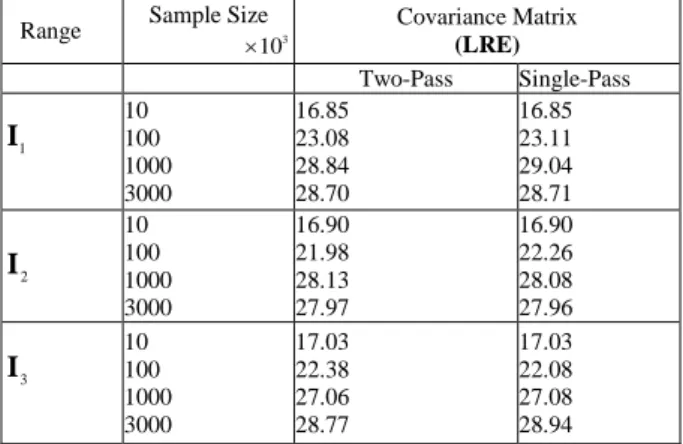
All experiments were performed using Hadoop version 1.0.4 on a small cluster of three machines: One 8 core 16 GB RAM and two 6 core 8 GB RAM each. Table I presents the LRE values obtained from the single-pass and the naive two pass algorithms. The results indicate that the single-pass is slightly more stable than the naive two-pass. For sample sizes greater than 3
3000 10 it became too costly to compute the naive two-pass covariance matrix on a single machine.
TABLEI:ACCURACY OF SINGLE-PASS AND TWO-PASS ALGORITHMS
Range Sample Size 3
10 Covariance Matrix (LRE) Two-Pass Single-Pass 1 I 10 100 1000 3000 16.85 23.08 28.84 28.70 16.85 23.11 29.04 28.71 2 I 10 100 1000 3000 16.90 21.98 28.13 27.97 16.90 22.26 28.08 27.96 3 I 10 100 1000 3000 17.03 22.38 27.06 28.77 17.03 22.08 27.08 28.94
TABLEII:ACCURACY OF LOCAL MODELS VS DISTRIBUTED MODEL
B. Effective Scale-Down Sampling Scheme
This section demonstrates the effectiveness of using uncertainties in LDA and LR as tools for down-sampling large data sets. Empirical results on two real large data sets are presented.
The basic idea is to apply Algorithms 1 and 2 and the Hausman's test on distributed data to select only the most informative examples for local learning. The algorithms also outputs the parameters of LDA and LR from which local learning and distributed learning can be compared.
C. Data Sets
The first real data set is the Airline data set (http://stat-computing.org/dataexpo/2009/) consisting of more than 120 million flight arrival and departure information for all commercial flights within the USA, from October 1987 to April 2008. The classification problem
D
Dataset Models Accuracy Training Size Training Time (min) Flight LDAd LRd SVMd 0.75 0.78 - 28,259,655 28,259,655 28,259,655 43.7 125.9 - LDAl LRl SVMl 0.73 0.77 0.77 587,079 40,154 40,154 45.3 126.3 137.4 Linkage LDAd LRd SVMd 0.98 0.99 0.98 4,311,849 4,311,849 4,311,849 10.81 25.6 786.47 LDAl LRl SVMl 0.98 0.99 0.99 110,078 20,328 20,328 15.81 27.6 32.7
formulated here is to predict flight delays. The data contained a continuous variable indicating flight delays in minutes where negative values meant flight was early and positive values represented delayed flights. A binary response variable was created where values greater than 15 min were coded as 1 and zero otherwise. Flights details for four years: 2004-2007 (n = 28,259,655) was used for training and details for 2008 (n = 5,810,461) reserved for testing.
The second data set is the Record Linkage Comparison Patterns data set from the UCI machine learning repository and consists of 5,749,132 record pairs. The classification task is to decide from comparison patterns whether the underlying (medical) records belongs to the same individual. The data set was split into 75% training and 25% testing.
Three classifiers: LDA, LR and SVM were trained on scaled down (local data) and their performance assessed on a large distributed test data. The three classifiers were equally trained on the full distributed data using MR and tested on the same test set. Due to the large sample size of the flight data, it was computationally very expensive to train SVM on the full data, so only the local results are available. An attempt was also made to perform an SVM sampling scheme on MapReduce, i.e select only the support vectors for learning. However, the approach was again computationally too expensive and was dropped. The Gaussian kernel was used for SVM with 5-fold cross-validation procedure for parameter selection. To differentiate a local model from distributed model the subscripts
l
andd
will be used respectively.The Airline and record linkage data sets contain binary and categorical variables with at least 3 levels clearly indicating non-normal conditions. This was verified by Hausman's test meaning that LR may be more robust to learn the data than LDA. However, LDA results will still be reported. With a 95% confidence interval, it was observed that the number of samples selected by both sampling schemes was usually less than 3% of the training size.
Table II shows the performance of LDA, LR and SVM models trained locally using sampled data selected by the LDA and LR sampling schemes compared to their performance on the full training set. The local LDA model is trained on data sampled by the LDA sampling scheme and likewise for the local LR model. However, because the LDA normal assumption was violated for both data sets, the SVM local model was trained on data selected by the LR sampling scheme. The training times for the local models in the last column is the total time to perform the scaled down operation on MR and to carry out local training of the classifiers on a single machine.
The results from Table II illustrates the effectiveness of the sampling schemes in terms of both accuracy and time scalability. While it was not possible to train SVM on the large flight data set, using the LR sampling scheme, it was possible to train SVM locally giving almost the same predictive accuracy as LR trained on the full data set. Equally for the record linkage data set, it took almost 13 hours to train the SVM classifier on MapReduce while an even better accuracy was obtained with less than 0.5% the training size in only about half an hour.
Training the classifiers on less than 3% of the original training size resulted in almost the same accuracy as leaning
from the complete data. This result illustrates the effectiveness of the sampling schemes. Though the LDA failed the Hausman's specification test, its overall performance was however very good.
VII.CONCLUSION
This paper presented three major contributions to research in machine learning with large distributed data sets. First, a general single pass formula for computing the covariance matrix of large distributed data sets was derived. Numerical results obtained from application of the new formula showed slightly more stable and accurate results than the traditional two pass algorithm. In addition, the presented formula does not require any pairwise incremental updating schemes as existing techniques. Second, two new simple, fast, parallel efficient, scalable and accurate sampling techniques based on uncertainties of the linear discriminant score and the logistic regression model were presented. These schemes are readily implemented on the MapReduce framework and makes use of the single-pass covariance matrix formula. With these sampling schemes, large distributed data sets can be scaled down to manageable sizes for efficient local processing on a single machine. Numerical evaluation results demonstrated that the approach is accurate and cost effective, producing results that are accurate as learning from the full distributed data set.
REFERENCES
[1] C. Chu, S. K. Kim, Y.-A. Lin, Y. Yu, G. Bradski, and A. Y. N. A. K. Olukotun, "Map-reduce for machine learning on multicore," Advances
in Neural Information Processing Systems, vol. 19, pp. 281, 2007.
[2] R. Bekkerman and M. Bilenko, and J. Langford, Scaling up machine
learning: Parallel and distributed approaches, Cambridge University
Press, 2011.
[3] F. Zhang, J. Cao, X. Song, and H. C. A. C. Wu, "Amref: An adaptive mapreduce framework for real time applications," in Proc. 2010 9th
International Conference on Grid and Cooperative Computing (GCC),
2010, pp. 157-162.
[4] B. Panda, J. S. Herbach, S. Basu, and R. J. Bayardo, "Planet: massively parallel learning of tree ensembles with mapreduce," Proceedings of
the VLDB Endowment, vol. 2, no. 2, pp. 1426-1437, 2009.
[5] J. Bennett, R. Grout, P. Pébay, D. Roe, and D. Thompson, "Numerically stable, single-pass, parallel statistics algorithms," in Proc.
IEEE International Conference on Cluster Computing and Workshops,
2009, pp. 1-8.
[6] A. W. Lo, "Logit versus discriminant analysis: A specification test and application to corporate bankruptcies," Journal of Econometrics, vol. 31, no. 2, pp. 151-178, 1986.
[7] B. Settles, "Active learning literature survey," University of Wisconsin, Madison, 2010.
[8] F. Critchley and I. Ford, "Interval estimation in discrimination: the multivariate normal equal covariance case," Biometrika, vol. 72, no. 1, pp. 109-116, 1985.
[9] A. Frank and A. Asuncion, "UCI machine learning repository,"2010. [10] P. J. Bickel and B. Li, Mathematical statistics, in Test, 1977. [11] A. C. Rencher and G. B. Schaalje, Linear models in statistics,
Wiley-Interscience, 2008.
[12] A. I. Schein and L. H. Ungar, "Active learning for logistic regression: an evaluation," Machine Learning, vol. 68, no. 3, pp. 235-265, 2007. [13] B. Efron, "The efficiency of logistic regression compared to normal
discriminant analysis," Journal of the American Statistical Association,
vol. 70, no. 352, pp. 892-898, 1975.
[14] C. Ngufor and J. Wojtusiak, "Learning from large-scale distributed health data: An approximate logistic regression approach," in Proc.
ICML 13: Role of Machine Learning in Transforming Healthcare,
2013.
[15] M. Zinkevich, M. Weimer, A. Smola, and L. Li, "Parallelized stochastic gradient descent," Advances in Neural Information
Processing Systems, vol. 23, no. 23, pp. 1-9, 2010.
[16] B. D. McCullough, "Assessing the reliability of statistical software: Part I," The American Statistician, vol. 52, no. 4, pp. 358-366, 1998.
Che Ngufor received his B.sc in mathematics and computer sciences from the University of Dschang, Cameroon in 2004, M.sc in mathematics from Tennessee Technological University, Cookevile, TN in 2008. He is currently working on his Ph.D in computational sciences and informatics at George Mason University, Fairfax, VA.
Mr. Ngufor's main research areas include computational mathematics and statistics, medical informatics, distributed and parallel computing, big data and large-scale machine learning and knowledge discovery.
Janusz Wojtusiak obtained his master's degree in computer science from Jagiellonian University in 2001, and Ph.D. in computational sciences and informatics (concentration in Computational Intelligence and Knowledge Mining) from George Mason University in 2007.
Currently Dr. Wojtusiak is an assistant professor in the George Mason University Department of Health Administration and Policy, and the coordinator of GMU Health Informatics program. He also serves as the director of the GMU Machine Learning and Inference Laboratory, and the director of GMU Center for Discovery Science and Health Informatics.