for Text Classification With SVMs
S. Sathiya Keerthi [email protected]
Yahoo! Research Labs, 210 S. DeLacey Avenue, Pasadena, CA-91105
Abstract
In this paper we generalize the LARS feature selection method to the linear SVM model, derive an efficient algorithm for it, and empir-ically demonstrate its usefulness as a feature selection tool for text classification.
1. Introduction
Text classification is an interesting collection of clas-sification problems in which the number of features is large that often exceeds the number of training ex-amples and, for which, linear classifiers such as lo-gistic regression (Genkin et al., 2004), linear SVMs (Joachims, 1998) and regularized least squares work very well. For these problems, feature selection can be important, either for improving accuracy or for reduc-ing the complexity of the final classifier. Filter meth-ods such as information gain (Yang & Pedersen, 1997) and bi-normal separation (Forman, 2003) are usually employed to do feature selection.
LARS (Least Angle Regression and Shrinkage) is a ‘semi-wrapper’1 feature selection approach devised by
Efron et al (Efron et al., 2004) for ordinary least squares. It is closely related to the Lasso model (Tib-shirani, 1996) which corresponds to the use ofL1
regu-larizer for least squares problems. The great advantage of LARS is its ability to order variables according to their ‘importance’, while keeping the total computa-tional cost small.
In this paper we generalize the LARS approach to lin-1
Unlike filter methods which order features by analyzing them independently, LARS sequentially chooses new fea-tures that are dependent on the feafea-tures that are already chosen, and is ‘wrapped around’ the induction algorithm. However, it is not a full-fledged wrapper method since it is only based on optimizing the training set performance. Appearing inProceedings of the 22ndInternational Confer-ence on Machine Learning, Bonn, Germany, 2005. Copy-right 2005 by the author(s)/owner(s).
ear SVMs, derive an efficient algorithm for it, along the lines of Rosset and Zhu’s path tracking algorithm for L1regularized models (Rosset & Zhu, 2004), and point
out that this algorithm is computationally practical, say for ordering and choosing the top 1000 features of a (binary) text classification problem. We evaluate the generalization performance (F-measure) on several text classification benchmark datasets and show that SVM with LARS generates an ordering of features that is much better than that obtained using information gain. Regularized least squares with LARS (Zou & Hastie, 2005; Efron et al., 2004) is also evaluated and shown to be inferior for text classification compared to SVM with LARS.
SVM with LARS can be viewed as an efficient approxi-mate algorithm for a modified SVM formulation which uses both, an L2 regularizer and an L1 regularizer.
(The algorithm essentially efficiently tracks the solu-tion curve for all possibleL1regularizer coefficient
val-ues.) As a part of our study we also evaluate the use-fulness of keeping (or leaving out) theL2 regularizer.
When the L2 regularizer is left out, the model with
LARS is close in spirit to the sparse logistic regression model recently proposed (and shown to be very good) by Genkin et al (Genkin et al., 2004) for text classi-fication. Keeping only the L1 regularizer leads to an
aggressive reduction of the training cost using a small subset of features. On some datasets this leads to an impressive performance while, on other datasets that need to keep a large number of features2 for optimal
performance, the aggressive feature removal property of theL1 regularizer (acting alone) leads to a loss in
performance. Thus, it is better to try both classifiers: one which keeps theL2regularizer and a second which
leaves out theL2regularizer, and choose the better one
based on validation.
The paper is organized as follows. Section 2 is the main section where the generalized LARS idea is explained and the SVM-LARS algorithm is derived. Section 3
2
The20 Newsgroups dataset is a good example of this case.
evaluates the various methods on 6 benchmark binary classification problems. Concluding remarks are given in section 4.
The following notations will be used in the paper. x0 will denote the transpose of the vector/matrix x. xj
is the j-th component of the vector x. Given a set
A, |A| will denote the cardinality of A. Forβ ∈Rm
and A ⊂ {1, . . . , m}, βA is theA dimensional vector
containing {βj, j ∈ A}. If q= maxp∈Ph(p) and ¯p=
arg maxp∈Ph(p), then we say ¯pdefinesq.
2. Generalized LARS Algorithm
Consider a (binary) classifier whose training can be expressed as
min
β f(β) (1)
wheref is the sum of a regularizer term and a data-fit term, and the parameter vectorβ is an element ofRm.
Let g(β) denote the gradient of f. We are interested in the following two models.
Model 1. Regularized Least Squares (RLS)3
f(β) =fRLS(β) = λ2 2 kβk 2+1 2 n X i=1 r2i(β) (2)
wherekβkis theL2norm ofβ,xiis thei-th example’s
input vector,ri(β) =β0xi−ti,ti ∈ {1,−1} is the
tar-get (1 denotes class 1 and -1 denotes class 2) for thei -th example, andnis the number of training examples.4
The gradient offRLSis: gRLS(β) =λ2β+X0(Xβ−t)
where X is the n×m matrix whose rows have {x0i}
andt is the target vector containing{ti}.
Model 2. SVM (with L2 loss)
f(β) =fSV M(β) = λ2 2 kβk 2+1 2 X i∈I(β) ri2(β) (3)
whereI(β) ={i:tiri(β)<0}and the other quantities
are as defined forfRLS. It is easy to check thatfSV M
is continuously differentiable and that its gradient is given by: gSV M(β) =λ2β+XI0(XIβ−tI) whereXI
is the matrix whose rows have{x0
i, i∈I(β)} andtI is
the vector containing{ti, i∈I(β)}.
SVM with hinge loss corresponds to replacing the r2i(β) term in (3) by −2tiri(β). When there are no
severe outliers in the training set, the SVM models using theL2 and hinge loss produce very similar
clas-sifiers. We work with L2 loss because our ideas for
3
The model is same as ridge regression on the classifier targets.
4
We assume throughout this paper that the bias term is built intoβand that it is also regularized.
feature selection only apply to models for which f is continuously differentiable. SVM with modified Huber loss, which also has this property, is another excellent alternative that can be used together with our LARS ideas. In this paper we will present our ideas only for theL2loss. By doing minor modifications, these ideas
can be easily extended to the modified Huber loss. Lasso (Tibshirani, 1996) and Elastic Net (Zou & Hastie, 2005) are feature selection tools that apply to fRLS. (Lasso is designed forλ2= 0.) They do
system-atic feature selection by including anL1regularizer in
the cost function:
min ˜f(β) =f(β) +λ1kβk1 (4)
where kβk1 is the L1 norm of β. When λ1 is large5
β = 0 is the minimizer of ˜f, which corresponds to the case of all variables being excluded. Asλ1is decreased,
more and more variables take positive values. When λ1 →0, the solution of (4) approaches the minimizer
off.
In the above approach, as λ1 is decreased, a βj can
move back and forth between zero and non-zero val-ues more than once. LARS is a closely related, but computationally much simpler approach that was de-vised by Efron et al (Efron et al., 2004) for ordinary least squares problems (i.e., fRLS with λ2 = 0); this
approach only keeps adding variables as a parameter similar toλ1 is decreased.6
The basic idea behind LARS is simple. Though not mentioned in Efron et al. (2004), LARS can be eas-ily extended to other models such as fSV M. We
will refer to the extension also as LARS. To under-stand the method, first note that β? is a minimizer
of f iff it is a (global) minimizer of the function gmax(β) = maxj|gj(β)|. LARS starts from β = 0
and continuously decreases gmax by adding variables
one at a time until β? is reached. At β = 0 let j 1
be the index which defines gmax. Takeβj1 as the first variable (at the current point it is the variable that contributes most to the decrease inf) to be included. Let sj1 = sgn(gj1(0)). If we start from λ1 =gmax(0)
and track the curve defined by gj1 = λ1sj1 with βj1
and λ1 as the only variables allowed to change, then
gmax can be decreased.7 This can be continued until
we reach a ˜λ1 and ˜β where another variable index j2
also definesgmax, i.e.,|gj2( ˜β)|=|gj1( ˜β)|= ˜λ1. At this
5
It is easy to see that, ifλ1>maxj|gj(0)|, then the
di-rectional derivatives of theλ1kβk1term atβ= 0 dominate
and soβ= 0 is the minimizer of ˜f.
6
Since we use only LARS in this paper, we will call this parameter for LARS also asλ1.
7
At any stage of the LARS algorithm λ1 equals gmax.
point LARS includesβj2 as the new variable for
inclu-sion and tracks the curve defined by the two equations, gj1 = λ1sj1, gj2 = λ1sj2, where sj2 = sgn(gj2( ˜β))
and, βj1,βj2 andλ1 are the only variables allowed to
change. The procedure is repeated to include more variables whilegmax is continuously decreased.
Because the choice of new variables is done conditional on variables already included, LARS has the potential to be better than filter methods which analyze fea-tures independently. Since the importance of variables is judged by the size of the derivative off, it is neces-sary to scale the variables uniformly. Most representa-tions employed in text classification (binary, normal-ized binary, normalnormal-ized tf-idf etc) have such a uniform scaling. They all give data values spread in the (0,1) range. Let us now give full details of the (generalized) LARS algorithm.
Algorithm LARS
1. Let ¯β = 0. Find ¯j = arg maxj|gj( ¯β)|. Let A= {¯j},s¯j = sgn(g¯j( ¯β)), ¯λ1=|g¯j( ¯β)|. Go to step 2.
2. Consider the curveP in (β, λ1) space defined by
P = {(β, λ1) :gj =sjλ1∀j∈ A, βk= 0∀k6∈ A, λ1≤¯λ1} (5) Find ˜ λ1 = sup{ λ1: (β, λ1)∈P, |gk| ≥λ1 for some k6∈ A } (6) Let the correspondingβ be ˜β. If ˜λ1 = 0, stop. If
˜
λ16= 0, then by continuity arguments there exists
˜
k 6∈ A for which |gk| = ˜λ1; obtain ˜k and go to
step 3.
3. LetA:=A ∪ {˜k}, ¯β = ˜β,s˜k= sgn(g˜k( ˜β)) and go
back to step 2.
Consider a generic stage of the algorithm at which ¯β satisfies ¯gj =sjλ1 ∀j ∈ Aand ¯βj = 0∀j 6∈ A. It is
easy to see that ¯β is the minimizer off−s0AβAwhere
onlyβA is varied, andsA is theAdimensional vector
containing{sj, j∈ A}.
Suppose we decide to run the algorithm only upto a point where dvariables have been chosen and so stop at the end of step 2 when |A| = d occurs. At that point what is the β that should be used as the pa-rameter vector for the classifier? One idea is to use β = ˜β. This is the parameter vector we have used in all the computational experiments reported in this pa-per. Since we are terminating the algorithm with only
a partial set of variables, g( ˜β)6= 0. We can take the d parameters defined by A, optimize f with respect to these parameters and obtain the parameter vector,
ˆ
β. This is another worthwhile possibility for use in the final classifier. For ordinary least squares (fRLS
with λ2 = 0), Efron et al (Efron et al., 2004) refer to
this alternative as the OLS/LARS hybrid. One can also think of fundamentally altering the algorithm by solving gj = 0, j ∈ A to obtain ¯β, j ∈ A, and then
choosing the next entering variable to be the one which has the largest magnitude gradient component. Such an aggressive forward selection scheme can be overly greedy, leading to a poor selection of features (Efron et al., 2004).
Let us now discuss the computer implementation of the above algorithm. Let us begin with f = fRLS
since the ideas are simpler for it. Although details for the least squares case are given in Efron et al. (2004) and Zou and Hastie (2005), we repeat them here since they smoothly lead us to the details for f = fSV M.
Let βA denote the|A| dimensional vector containing
{βj, j∈ A}. Forf =fRLS, thegj are affine functions
ofβAand soP is a linear curve. The direction of that
linear curve, δβA can be determined by solving the
linear system,
HAδβA=sA (7)
where: HA = λ2I|A|+XA0 XA; I|A| is the identity
matrix of size|A|;XAis then× |A|submatrix of the
data matrixX corresponding to the variables defined by A; and sA is a |A| dimensional vector containing
{sj, j∈ A}. The computational algorithm can now be
easily given. By the way δβA is defined in (7) note
thatβAhas to be moved in the negativeδβAdirection
in order to decreaseλ1.
Algorithm RLS-LARS
1. Let ¯β = 0. Compute ¯g = −X0t and find ¯j = arg maxj|g¯j|. Let A ={¯j}, s¯j = sgn(¯g¯j), ¯λ1 = |g¯¯j|,L=
√
HAwhereHA=λ2+XA0 XA. (SinceA
is a singleton, HA is a real number. Throughout
the algorithm L will denote the lower triangular Cholesky factorization ofHA.) Go to step 2.
2. (a) Solve LL0δβ
A = sA (two triangular linear
systems) to get the direction vector δβA.
Then compute δg = X0X
AδβA, the change
ing caused byδβA.
(b) For eachk6∈ A: solve ¯gk+ (λ1−λ¯1)δgk =λ1
to getλ+1k; solve ¯gk+ (λ1−λ¯1)δgk=−λ1 to
get λ−1k; and then set ˜λ1k = min+{λ˜+1k,˜λ
−
1k}
where min+ means that, when the minimum
λ1is decreased from ¯λ1andP is tracked, ˜λ1k
is the first λ1 value at which |gk| = λ1
oc-curs.)
(c) Let ˜λ1 = max{˜λ1k : k 6∈ A} and ˜k be the
k which defines ˜λ1. (IfA={1, . . . , m} then
simply set ˜λ1 = 0; in this case, ˜k is
unde-fined.) Go to step 3.
3. Reset ¯βA := ¯βA+ (˜λ1−¯λ1)δβA, ¯g := ¯g+ (˜λ1−
¯
λ1)δg, and ¯λ1 := ˜λ1. If ˜λ1 = 0 stop. Else, set A:=A ∪ {˜k},s˜k = sgn(¯g˜k), incrementally update
the cholesky factorLto include the new variable and go back to step 2.
In text classification problems the number of variables is large and so the above algorithm will be imprac-tical if a complete ordering of the full set variables is to be carried out. But, there is rarely a need to run the above algorithm beyond the selection of about 500-1000 top variables. In many cases the classifier performance peaks within that selection; if the perfor-mance continues to rise even beyond, that is usually an indication that using the full set of variables is the best way to go. Therefore it is sufficient to run the algorithm till about 500-1000 variables are chosen. Let us do a complexity analysis for an early termina-tion of the algorithm when it is run tilldvariables are chosen. Let mA = |A| and nnz denote the number
of non-zero elements in X. In textual problems X is usually very sparse and so nnz is a small fraction of
nm(which is the value ofnnz for a denseX matrix).
For our analysis we can take n and m to be smaller thannnz. The main cost of the algorithm is associated
with steps 2(a) and (3), which respectively have the complexities, O(m2
A+nnz) and O(m2A).
Accumulat-ing uptodvariables we get the algorithm’s complexity upto d variables as O(d3+nnzd). To get an idea of
the times involved, take a problem with about 10,000 examples having 100 non-zero elements in each exam-ple, i.e., nnz is about 1 million. If d = 1000 thend3
and nnzdare about the same order and so the
over-all cost of running the algorithm upto 1000 variables is only about few times the cost of inverting a 1000 dimensional dense square matrix.
Let us now turn to the extension of the algorithm to SVM. For fSV M, thegj are piecewise-affine functions
of βA and so the curve P in (5) is piecewise-linear.
Rosset and Zhu (Rosset & Zhu, 2004) discuss a range of models for which the overall curve parametrized with respect toλ1is piecewise-linear. Though they do
not explicitly includefSV Min their list of such models,
all their ideas can be easily extended tofSV M too. Let
us now take up these details. Apart from identifying
λ1values at which a new variable enters, we also need
to locate points at which an example leaves or enters the active index set, I. The following algorithm gives all the details. Many of the steps are same as those in algorithm RLS-LARS. In the algorithm we use yi to
denotetiri; thus, yi<0 means thati∈I.
Algorithm SVM-LARS
1. Let ¯β = 0, I = {1, . . . , n} and ¯yi = −1,
i = 1, . . . , n. Compute ¯g = −X0t and find ¯
j = arg maxj|g¯j|. Let A = {¯j}, s¯j = sgn(¯g¯j),
¯
λ1 = |g¯¯j|, L = √
HA where HA =λ2+XA0 XA.
Go to step 2.
2. (a) SolveLL0δβA=sAto get the direction
vec-tor δβA. Then compute δr = XAδβA, and
then,δg=X0δr.
(b) For eachk6∈ A: solve ¯gk+ (λ1−λ¯1)δgk =λ1
to getλ+1k; solve ¯gk+ (λ1−λ¯1)δgk=−λ1 to
getλ−1k; and then set ˜λ1k = min+{˜λ+1k,λ˜
−
1k}.
(c) Let ˜λ1 = max{λ˜1k, k 6∈ A} and ˜k be the k
which defines ˜λ1. (If A = {1, . . . , m} then
simply set ˜λ1 = 0; in this case, ˜k is
unde-fined.)
(d) For each i = 1, . . . , n, compute δyi = tiδri
andλ1i, the solution of ¯yi+ (λ1−¯λ1)δyi= 0.
(As βA is changed from ¯βA along the line
defined by the δβA direction, λ1i is the λ1
value at which the i-th example will hit the margin plane corresponding to it.)
(e) Find ˆλ1a, the first λ1 ≤ ¯λ1 at which an
example from group I moves out of I, i.e., ˆ
λ1a = max{λ1i : i ∈ I, δyi < 0}. Let ˆia be
thei∈Ithat defines ˆλ1a. (If, either ˆλ1a<0
or 6 ∃ i ∈ I such that δyi < 0, then simply
reset ˆλ1a = 0. For this case, the value of ˆia
is immaterial and can be left undefined.) (f) Find ˆλ1b, the firstλ1≤λ¯1at which an
exam-ple from outside group I moves into I, i.e., ˆ
λ1b = max{λ1i : i 6∈ I, δyi > 0}. Let ˆib be
thei6∈I that defines ˆλ1b. (If, either ˆλ1b<0
or 6 ∃ i 6∈ I such that δyi > 0, then simply
reset ˆλ1b= 0. For this case, the value of ˆib is
immaterial and can be left undefined.) (g) If ˆλ1a ≥ ˆλ1b then set ˆλ1 = ˆλ1a, ˆi = ˆia; else
set ˆλ1= ˆλ1b, ˆi= ˆib;
(h) If ˜λ1≥λˆ1 go to step 3; else go to step 4.
3. Reset ¯βA := ¯βA+ (˜λ1−¯λ1)δβA, ¯y := ¯y+ (˜λ1−
¯
λ1)δy, ¯g:= ¯g+(˜λ1−λ¯1)δg, and ¯λ1= ˜λ1. If ˜λ1= 0
incre-mentally update the cholesky factor Lto include the new variable and go back to step 2.
4. Reset ¯βA := ¯βA+ (ˆλ1−¯λ1)δβA, ¯y := ¯y+ (ˆλ1−
¯
λ1)δy, ¯g:= ¯g+(ˆλ1−λ¯1)δg, and ¯λ1= ˆλ1. If ˆλ1= 0
stop. Else, do the following. If ˆi ∈ I, remove ˆi from I, incrementally update the cholesky factor L(see text below) to remove the effect of example ˆi; else, include ˆi in I, incrementally update the cholesky factorL (see text below) to include the effect of example ˆi. Go back to step 2.
The Cholesky update in step 4 can be implemented as follows. Let ˆxbe the |A| dimensional vector formed by taking the ˆi-th example, xˆi and keeping only the
elements corresponding to A. Then the update corre-sponds to forming the Cholesky factors of LL0±xˆxˆ0.
This can be accomplished inO(|A|2) effort.
Though the complexity of one loop of steps 2-4 of SVM-LARS is same as the complexity of one loop of steps 2-3 of RLS-LARS, the overall complexity of SVM-LARS is higher than that of RLS-LARS due to the number of loops executed. Typically, examples only move out of I as the algorithm proceeds (note that, at the beginning,I={1, . . . , n}). For our analy-sis here, let us assume that this is true. Letnch be the
number of examples that move out of I by the time d variables have been included. The total number of loops of steps 2-4, then, is d+nch. The total cost of
the algorithm is bounded by O((nnz+d2)(nch+d)).
Letnsvdenote the number of support vectors (i.e.,|I|)
in the SVM which uses all the variables. Then we have nch≤(n−nsv). This bound gives us a good estimate
ofnch.
For problems in which nch is large (nsv is small)
the extra cost of SVM-LARS over RLS-LARS (i.e., O((nnz+d2)nch)) can be big. There is a simple way
to reduce this extra cost considerably while bringing in some approximateness to the algorithm that is not serious. For lack of space, we skip all these details here. We have also developed an efficient method for tracking an approximation of the leave-one-out error as a function ofλ1. For lack of space we skip these
de-tails too. This approximation serves well for selecting the number of features to use.
3. Empirical Analysis
In this section we empirically evaluate the usefulness of LARS as a feature selection tool for SVM and RLS, and, in the process, also compare SVM and RLS as well as study the usefulness of keeping (or leav-ing out) the L2 regularizer term in f. Although we
have conducted the evaluation on many datasets, here we only report representative results on the following datasets.8
• Fbis-4: 1 binary problem of theFbis dataset cor-responding to class 4 (with 387 examples) against the rest;n= 2463;m= 2000.
• La1-2, La1-4: 2 binary problems of the La1 dataset corresponding to class 2 (with 555 exam-ples) and class 4 (with 943 examexam-ples) against the rest;n= 3204;m= 31472.
• Ohscal-7: 1 binary problem if theOhscal dataset corresponding to class 7 (with 1037 examples) against the rest;n= 11162;m= 11465.
• Reuters-Money-fx : 1 binary problem of the Reutersdataset corresponding to the class money-fx (with 717 examples) against the rest; n = 12902;m= 37207.
• News-3 : 1 binary problem of the 20 News-groupsdataset corresponding to class 3 (with 1000 examples) against the rest; n = 19928; m = 62061.
All these problems have a reasonably rich number of examples in each class. We study generalization per-formance as a function of the number of features. F-measure is used as the generalization performance met-ric. To evaluate the set of features obtained by LARS we compare it (in terms of the F-measure) against the set of features obtained by ordering according to in-formation gain (IG).9
The following six methods were compared: SVM-LARS (λ2= 1); SVM-LARS (λ2= 0); SVM-IG;
RLS-LARS (λ2 = 1); RLS-LARS (λ2 = 0); and, RLS-IG.
Note that, setting λ2 = 0 with SVMs does define a
meaningful model since the L1 regularizer is present.
For RLS, setting λ2 = 0 corresponds to the Lasso
model (Tibshirani, 1996). For the case of non-zeroλ2,
we did not tune λ2, mainly to keep the computations
8
Fbis, La1 and Ohscal, which use binary representa-tion for the words, are as in Forman (2003). TheReuters
dataset is taken from (Lewis, 2004) and20 Newsgroups is as in Rennie and Rifkin (2001). For these two datasets we use normalized tf-idf representation.
9
One could also consider other good filter methods such as BNS (Bi-Normal Separation) (Forman, 2003). We tried BNS, but it did not perform as well as IG on the datasets chosen by us. This is not inconsistent with the findings of Forman (Forman, 2003) who found BNS to be better, overall, on a range of problems in which many had large class skew. The binary problems chosen by us do not have big class skew.
manageable; also, it has been generally observed that, for text classification problemsλ2= 1 is a good choice
that gives a performance close to optimal. For each classifier used in our study we do a post-processing tuning of the threshold to optimize the F-measure. The validation outputs needed for doing this were ob-tained using the LOO approximation mentioned in sec-tion 2 for LARS and using 10-fold cross validasec-tion for IG ordering.10
Since the training set/testing set split can cause vari-ability that needs to be shown for a proper compari-son of the methods, we set-up the comparicompari-son exper-iments as follows. Each binary dataset was randomly divided into 4 (classwise stratified) groups; 4 runs were made, each time keeping one group as the testing set and the remaining 3 groups as the training set. Thus, for each classifier method and a given number of fea-tures selected, we get 4 F-measure values as estimates of generalization performance. Let Fmin, Fmean and
Fmax denote the minimum, mean and maximum of
these four values. The experiment was repeated for 10 different choices of the random 4-groupings; Fmin,
Fmean and Fmax were averaged over the 10 runs to
get the averaged values,avFmin,avFmeanandavFmax.
While avFmean gives an estimate of the expected
F-measure value,avFmax−avFmin gives us an estimate
of its variability. For each method, we plot avFmin,
avFmean and avFmax as a function of the number of
features chosen. The analysis was done upto a max-imum of 2000 chosen features. We also ran SVM and RLS using all the features in a given dataset and λ2 = 1 to get another baseline for comparison.
Only for the Reuters−Money−fx dataset, we did not form any random groupings; going by standard practice for the Reuters dataset, we simply use the ModApte train/test split once.
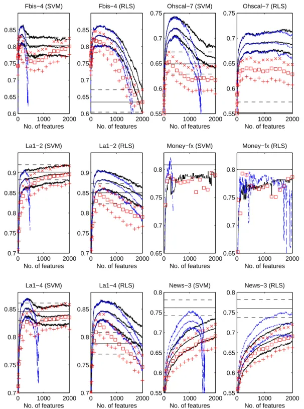
For the six binary problems and the various methods, Figure 1 gives plots of the F-measure statistics as a function of the number of features chosen. For the LARS approaches, the number of features is a non-linear scaling ofλ1. (Note that, asλ1 decreases more
features get included.) Also, since features are sequen-tially added one at a time, the performance values for LARS are available for every integer value of the num-ber of features. Since we are using F-measure, bigger values mean better performance. For the IG ordering we fixed λ2= 1 and only did the experiments for the
following values of the number of features: 2, 4, 8, 16, 32, 64, 128, 200 +k∗150, k = 0,1, . . . ,12. Figure 1
10
Like Genkin et al (Genkin et al., 2004) one could also simply use the training outputs to adjust the threshold. This will reduce the computational cost, but the perfor-mance of the chosen threshold will be slightly inferior.
also gives the statistics associated with the classifier which uses all features and hasλ2= 1.
We can group the findings under three headings. LARS versus IG.Although the initial, small set of features chosen by IG is very good (sometimes these initial features are even quite better than those cho-sen by LARS), LARS usually does much better in the middle phase where the performance either peaks or is approaching the peak. This superiority is very strik-ing in some cases; see, for instance, the performance on Ohscal-7. In several cases, peak performance is attained only when the number of features chosen is very large. Even in such problems, LARS usually does much better in pointwise comparison at various values of the number of features. This win makes LARS to be very useful in situations where there is a need to build classifiers using only a restricted number of features. La1-2 is one such case.
SVM versus RLS.In many cases, the performance of RLS is severely degraded by the inclusion of a large number of features. This is regardless of whether LARS or IG was used for feature selection. Rarely, a lesser degree of such degradation occurs with SVM too (see Ohscal-7, for instance). In terms of the peak performance achieved, SVM usually did quite better; also, SVM achieved the peak with less number of fea-tures.
Keeping (λ2 = 1) versus Leaving out (λ2 = 0)
the L2 regularizer. In the initial phase of feature
selection, the two classifiers are usually identical. This is because, in this phase, the data-fit term gets the maximum importance. After the gradient of the data-fit term has reached small values, the classifier with the L2 regularizer term concentrates on bridging the
effects of the regularizer term and the data-fit term, while the classifier without the L2 regularizer term
continues to pick up features to aggressively reduce the gradient of the data-fit term towards zero, leading to overfitting and a severe loss in generalization perfor-mance. It can also be seen that the number of features at which theλ2= 0 classifier falls to low values is
gen-erally much smaller for SVM than for RLS. This can be easily explained by the fact that, while RLS always concentrates on all the examples, the SVM only has to fit the active examples (the elements ofI) in its ‘least squares’ process. Thus the SVM can achieve this fit using much less features.
In some cases, peak generalization performance is achieved in the initial phase of feature selection itself; see Fbis-4, for instance. In such cases the absence of the L2 regularizer is harmless. But, in several cases
(see the SVM case in La1-2, for example) the perfor-mance of the classifier with the L2 regularizer keeps
rising as more features are added. For such problems, leaving out theL2regularizer is clearly a poor choice.
There are also some interesting cases ( Reuters-Money-fx ; News-3 ) where, in the initial phase of feature selection, leaving out the L2 regularizer gives much
better performance.11 Genkin et al (Genkin et al.,
2004) obtained very good results on the Reuters’ bi-nary problems using their logistic regression method with the L1 regularizer. Our LARS method
corre-sponding to leaving out theL2regularizer is very
sim-ilar to their method; the two methods mainly differ in the loss function employed and the way λ1 is tuned.
Our experiments indicate that it is safer to try, both λ2 = 1 and λ2 = 0, and choose the better one, say,
based on cross validation.
4. Conclusion
In this paper we applied generalized LARS to lin-ear SVMs and showed that this leads to effective fea-ture selection. SVM-LARS is close in spirit to an SVM model in which both, L2 and L1 regularizers
are present. An important advantage of the SVM-LARS algorithm is its ability to finely track the solu-tion with respect to λ1 without losing efficiency. The
model without theL2regularizer is also an interesting
model that is worth considering. We are working on developing an efficient algorithm for applying gener-alized LARS to logistic regression. For this case, the solution curve with respect toλ1is a nonlinear curve,
and hence the algorithmic aspects are more challeng-ing.
In our empirical study we used only the standard ‘Bag-Of-Words’ (BOW) representation for forming the tures. It is also possible to include other derived fea-tures, say, the distributional word cluster features con-sidered by Bekkerman et al (Bekkerman et al., 2003), who found that their cluster representation is better than that of BOW on some datasets, but worse on others. By putting the BOW features and the derived features together and using LARS to do feature selec-tion, there is hope for getting the best properties of both representations.
11
This can be very useful in situations where there is a need to work with a limited number of features. But, if that is not the case, keeping the L2 regularizer could
be the better option. Note, for example, in the case of
News-3 that, the performance of theL2 regularizer using
all features is much better than the peak performance of the classifier withλ2= 0.
References
Bekkerman, R., El-Yaniv, R., Tishby, N., & Winter, Y. (2003). Distributional word clusters vs. words for text categorization. Journal of Machine Learning Research,3, 1183–1208.
Efron, B., Hastie, T., Johnstone, T., & Tibshirani, R. (2004). Least angle regression. Annals of Statistics, 32, 407–499.
Forman, G. (2003). An extensive empirical study of feature selection metrics for text classification. Jour-nal of Machine Learning Research,3, 1289–1305. Genkin, A., Lewis, D. D., & Madigan, D. (2004).
Large-scale bayesian logistic regression for text cat-egorization.
Joachims, T. (1998). Text categorization with support vector machines: Learning with many relevant fea-tures.Proceedings of the Tenth European Conference on Machine Learning (ECML)(pp. 137–142). Lewis, D. D. (2004). Reuters-21578 text
cat-egorization test collection: Distribution 1.0 readme file (v 1.3) (Technical Report). www.daviddlewis.com/resources/.
Rennie, J. D. M., & Rifkin, R. (2001).Improving mul-ticlass text classification with the support vector ma-chine(Technical Report). Artificial Intelligence Lab, MIT.
Rosset, S., & Zhu, J. (2004). Piecewise linear regular-ized solution paths.
Tibshirani, R. (1996). Regression shrinkage and selec-tion via the lasso. Journal of the Royal Statistical Society, B,58, 267–288.
Yang, Y., & Pedersen, J. O. (1997). A comparative study on feature selection in text categorization. Proceedings of the 14th International Conference on Machine Learning(pp. 412–420).
Zou, H., & Hastie, T. (2005). Regularization and vari-able selection via the elastic net. Journal of the Royal Statistical Society, B.
0 1000 2000 0.6 0.65 0.7 0.75 0.8 0.85 No. of features Fbis−4 (SVM) 0 1000 2000 0.6 0.65 0.7 0.75 0.8 0.85 No. of features Fbis−4 (RLS) 0 1000 2000 0.7 0.75 0.8 0.85 0.9 No. of features La1−2 (SVM) 0 1000 2000 0.7 0.75 0.8 0.85 0.9 No. of features La1−2 (RLS) 0 1000 2000 0.7 0.75 0.8 0.85 No. of features La1−4 (SVM) 0 1000 2000 0.7 0.75 0.8 0.85 No. of features La1−4 (RLS) 0 1000 2000 0.55 0.6 0.65 0.7 0.75 No. of features Ohscal−7 (SVM) 0 1000 2000 0.55 0.6 0.65 0.7 0.75 No. of features Ohscal−7 (RLS) 0 1000 2000 0.65 0.7 0.75 0.8 No. of features Money−fx (SVM) 0 1000 2000 0.65 0.7 0.75 0.8 No. of features Money−fx (RLS) 0 1000 2000 0.55 0.6 0.65 0.7 0.75 0.8 No. of features News−3 (SVM) 0 1000 2000 0.55 0.6 0.65 0.7 0.75 0.8 No. of features News−3 (RLS)
Figure 1.F-measure, as a function of the number of features chosen, for the six binary problems. For each problem there are two plots: the left one has the SVM results and the right one has the RLS results. In each plot, theavF-measure values of LARS withλ2= 1 are given as continuous (black) lines and the avF-measure values of LARS withλ2= 0 are given by
(blue) broken lines. TheavFmin,avFmean andavFmaxvalues for the IG ordering withλ2 = 1 are respectively shown by
the (red) symbols, +, and×. TheavFmin andavFmax values for the classifier withλ2 = 1, using all the features are
shown by dotted (black) horizontal lines; the corresponding avFmean value is shown by a continuous horizontal (black)